Collective dynamics of the high-energy proton-nucleus collisions

Abstract

We analyze the proton-lead collisions at the LHC energy of $\sqrt{s_{NN}}=5.02$ TeV in the three-stage approach, previously used to successfully describe the relativistic A-A collisions. The approach consists of the early phase, modeled with the Glauber model, the event-by-event viscous 3+1 dimensional (3+1 D) relativistic hydrodynamics, and the statistical hadronization at freeze-out. We show that features typical of collective dynamics, such as the harmonic flow and the ridge structures in the two-particle correlations in relative azimuth and pseudorapidity, may be naturally explained in our framework. In the proton-nucleus system the harmonic flow is generated from an initially event-by-event deformed system and is entirely due to these initial fluctuations. Notably, fluctuations of strength of the initial Glauber sources which yield the observed distribution of hadron multiplicities and, at the same time, lead to correct values of the elliptic flow coefficients both from the two- and four-particle cumulant method, as measured by the ATLAS collaboration. The azimuthally asymmetric flow is not modified significantly when changing the viscosity coefficient, the initial time for the collective expansion, or the initial size of the fireball. The results present an estimate of the collective component in the two-particle correlations measured experimentally. We demonstrate that the harmonic flow coefficients can be experimentally measured with methods based on large rapidity gaps which reduce some of the other sources of correlations.

I Introduction

The recent interest in proton-nucleus (p-A) collisions stems from the expectations that the experimental data for this system could be used to test various theoretical approaches developed for relativistic collisions Salgado:2011pf , moreover, it could serve as a reference for experiments involving nucleus-nucleus (A-A) collisions. An interesting possibility is that the collective behavior clearly seen in the A-A collisions may be present already in the p-A collisions, and even in the proton-proton (p-p) collisions of highest multiplicity of the produced particles. The experimental ALICE:2012xs ; ALICE:2012mj ; CMS:2012qk ; Abelev:2012cya ; ATLAS:pPb ; Adare:2013piz ; Khachatryan:2010gv and theoretical Luzum:2009sb ; *d'Enterria:2010hd; *Bozek:2009dt; *CasalderreySolana:2009uk; *Avsar:2010rf; Bozek:2010pb ; *Werner:2010ss; Bozek:2011if ; Bozek:2012gr ; Shuryak:2013ke investigations can provide a limit on the amount of the collective flow in small systems, setting a boundary on the collective behavior and helping to answer the questions: How small may the system be and under what conditions it is still describable with hydrodynamics? What observables are most sensitive to the collectivity? What is the interplay of various stages of the dynamics, starting from the initial condition, through the intermediate evolution, to hadronization?

The studies of the A-A collisions at RHIC Arsene:2004fa ; *Adcox:2004mh; *Back:2004je; *Adams:2005dq and the LHC Collaboration:2011yba ; *Li:2011mp; *collaboration:2011hfa led to by now conventional interpretation of numerous observed phenomena in the mid-rapidity region via formation of a hot dense medium – the strongly interacting quark-gluon plasma – which evolves as a fluid and may be successfully described with relativistic hydrodynamics Teaney:2009qa ; *Broniowski:2008vp; *Shen:2011zc; *Schenke:2011zz; *Luzum:2011mm; *Ollitrault:2012cm; *newreview. Basic phenomena supporting this view are

• The harmonic flow (elliptic, triangular, higher-order) Ollitrault:1992 ; Alver:2010gr ; Arsene:2004fa ; Collaboration:2011yba

• Characteristic ridge structures seen  Alver:2008aa ; *Abelev:2009af; *ATLAS:2012at; *Aamodt:2011by; *Agakishiev:2011pe; *Chatrchyan:2011eka; CMS:2012qk ; Li:2011mp in the 2-particle correlation functions in relative pseudorapidity and azimuth, possible to explain with harmonic flow Voloshin:2004th ; *Takahashi:2009na; *Luzum:2010sp; *Sorensen:2011hm; *Werner:2012xh; Bozek:2012en .

• Specific features of the interferometric radii Abelev:2009tp ; Aamodt:2011mr .

• Jet quenching (see, e.g., Betz:2012hv and references therein).

In the study presented in this article we investigate the first two items from the above list for the case of the p-Pb collisions, recently studied at the LHC at the collision energy of $\sqrt{s_{NN}}=5.02$ TeV. We apply a treatment based on hydrodynamics to find quantitative estimates for the measured quantities, extending an early analysis of flow Bozek:2011if by one of us (PB) in the p-A and deuteron-nucleus systems, as well as the more recent event-by-event studies of the correlation functions Bozek:2012gr and the interferometric radii Bozek:2013df . As will turn out, our results agree at a quantitative or semi-quantitative level with the experimental data for the highest centrality classes, supporting the collective picture of the most central p-Pb collisions. Our results also set the background for more elementary explanations of the correlation studies, based on saturation and the color-glass-condensate (CGC) theory Dusling:2012iga ; Dusling:2012wy ; Dusling:2012cg ; Kovchegov:2012nd ; Kovner:2012jm ; Dusling:2013oia . We note that certain features can also be obtained with cascade models Lin:2004en ; *Solanki:2012ne; *Xu:2011fe; *Burau:2004ev.

We note that a certain degree of collectivity has been suggested for the p-p collisions as well Luzum:2009sb ; *d'Enterria:2010hd; *Bozek:2009dt; *CasalderreySolana:2009uk; *Avsar:2010rf; Bozek:2010pb ; *Werner:2010ss, where a same-side ridge is observed in the 2D correlations functions Khachatryan:2010gv for the highest multiplicity events. This may indicate the presence of azimuthal correlations in the gluon emission from the initial state Dusling:2012iga ; Dusling:2012wy ; Kovchegov:2012nd ; Kovner:2012jm ; Dusling:2013oia . However, the same-side ridge observed in the p-p collisions could also result from the collective expansion of the created medium Bozek:2010pb ; *Werner:2010ss. The intriguing questions concerning the p-p collisions will not be explored in this work, devoted to the detailed analysis of the p-Pb case.

Finally, we stress that our method is applicable to soft physics, related to particles produced with transverse momenta lower than, say, 2 GeV.

II The three-stage approach

Our event-by-event approach is based on, by now, a standard picture involving three stages: generation of the initial densities, hydrodynamic evolution, and hadronization. Certainly, variants of the modeling of each stage are present in the literature. We use the Glauber approach as implemented in GLISSANDO Broniowski:2007nz to model the initial phase, the 3+1 D viscous hydrodynamics Bozek:2011ua , and the statistical hadronization as implemented in THERMINATOR Kisiel:2005hn ; *Chojnacki:2011hb.

II.1 Initial conditions

The initial condition is generated with GLISSANDO Broniowski:2007nz , implementing various variants of the Glauber model Glauber:1959aa ; *Czyz:1969jg; *Bialas:1976ed; *Bialas:2008zza; Broniowski:2007ft . The parameters of the calculations are similar as in Bozek:2011if , except that they are adjusted for the collisions energy of $\sqrt{s_{NN}}=5.02$ TeV. Thus we take the nucleon-nucleon (NN) inelastic cross section $\sigma_{NN}=67.7$ mb, moreover, we use a realistic (Gaussian) wounding profile Rybczynski:2011wv for the NN collisions.

In the Glauber model, when a NN collision occurs, a source is produced, meaning a deposition of energy in a location in the transverse plane and spatial rapidity. In the standard wounded nucleon model it is assumed that a point-like source is located at the center of each participating nucleon, which leads to a rather large initial transverse size in the p-Pb system. Locating the source in the center-of-mass of the NN pair is also a possible model choice; it leads to smaller initial distributions. In the results presented below we use both variants of the model, termed standard and compact. That way we may estimate the uncertainty related to modeling the initial phase within the Glauber treatment.

There is another important effect in the initial stage that influences the results: The weight of each source fluctuates according to some statistical distribution, simply reflecting the fact that each NN collision may produce a different number of partons and therefore lead to varying deposition of the entropy. In the simulations Broniowski:2007nz , this feature is achieved by overlaying a suitable distribution of strength $w$ over the spatial distribution of the participant nucleons. As described in Sect. II.5, the observed multiplicity distributions can be described as convolution of the number of participant nucleons and a negative-binomial distribution. At the stage of the formation of the initial fireball it is equivalent to imposing fluctuations of the entropy deposited per participant nucleon following the $\Gamma$ distribution,

$$P_{\Gamma}(w)=\frac{w^{\kappa-1}\kappa^{\kappa}}{\Gamma(\kappa)}e^{-\kappa w}$$ (1)

with $\kappa=0.9$, as it leads to correct multiplicity distribution of the produced particles, cf. Sec. II.5. This case is labeled Glauber+NB as it eventually gives the multiplicity distribution as a convolution of the Glauber Monte-Carlo distribution of participant nucleons and a negative binomial distribution. It is the most physical one and leads to best results when compared to the experiment. By construction, in the Glauber+NB case we place the sources at the centers of the participant nucleons, as in the standard case.

In all cases, after generating the spatial positions of sources, we smooth them with a Gaussian profile of width 0.4 fm. This physical effect (the sources do have a non-zero width) is also essential for hydrodynamics, which requires sufficient smoothness of the initial conditions. The smoothed initial distribution is placed on the 3+1 D lattice with spacing of 0.15 fm and then the event-by-event hydrodynamics is run.

Table 1: The mean values and standard deviations of the basic characteristics of the initial distributions for the centrality class 0-3.4%.

	standard		compact		Glauber+NB
	mean	std. dev.	mean	std. dev.	mean	std. dev.
$\langle r^{2}\rangle^{1/2}$ [fm]	1.54	0.15	0.93	0.06	1.45	0.22
$\epsilon_{2}$	0.25	0.13	0.19	0.09	0.34	0.16
$\epsilon_{3}$	0.29	0.13	0.18	0.09	0.32	0.15

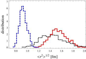
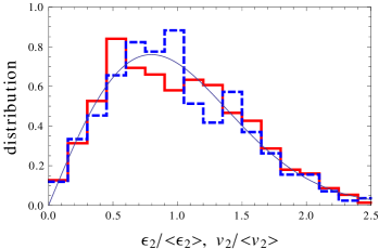
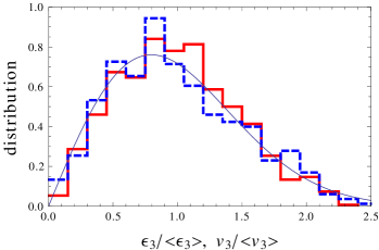
Some features of the resulting initial distributions are shown in Figs. 1 and 2 for the collisions at the high centrality, $c$=0-3.4%. We use here a few hundred configurations generated with GLISSANDO which are later fed into the event-by-event hydrodynamic evolution. The basic properties of the distributions are listed in Table. 1.

Figure 1: (Color online) The distribution of the transverse rms radius for the initial configuration in the standard case (solid line), compact case (dashed line), and the Glauber+NB case (dotted line), for the centrality class 0-3.4%.

Figure 2: (Color online) The distributions of the scaled eccentricities $\epsilon_{n}$ and scaled harmonic flow coefficients $v_{n}\{2\}$, $n=2,3$ for the standard case. The thin solid line shows the Wigner distribution of Eq. (4). The flow coefficients $v_{n}\{2\}$ are discussed in the following sections.

II.2 Initial size

At first glance, a rather surprising feature is the large transverse rms size of the initial distributions. To understand, consider first the standard case, where the sources are located in the centers of the proton and of each of the participants from the lead nucleus. If the geometric “hard-disk” of radius $R$ were used for wounding, then the inelastic cross section would be $\sigma_{NN}=\pi R^{2}$, from where $R=1.47$ fm, corresponding to rms of 0.98 fm in a single NN collision. This would be the uncertainty of the location of the point-like source created in the NN collision in the model. However, we use the realistic Gaussian wounding profile Rybczynski:2011wv of the form

$$p(b)=A\exp(-\pi Ab^{2}/\sigma_{NN}),\;\;A=0.92.$$ (2)

After folding with the distributions of the nucleons in the Pb nucleus (via the Monte Carlo procedure in GLISSANDO) and after smoothing the positions with Gaussians of width 0.4 fm located in the centers of each source, we obtain the rms radius of the initial distribution listed in Table 1, namely 1.54 fm.

In the compact case, where the the sources are placed in the center-of-mass of the colliding proton and the nucleon from the Pb nucleus, the source is significantly smaller, with the transverse rms of 0.93 fm. More involved models of the initial stage have been considered Dumitru:2012yr ; *Tribedy:2010ab; *Moreland:2012qw; *Schenke:2012hg. The details of the energy deposition, such as the fluctuations and small scale structures, are relatively more important in p-Pb than in A-A collisions. Our calculation, which uses two cases with significantly different initial size of the fireball can serve as an illustration of the effects of the variation in initial size on the final harmonic flow observables.

II.3 Initial eccentricities

The participant eccentricities shown in Figs. 2 are defined in the usual way for a given event as

$$\epsilon_{n}e^{i\Psi_{n}}=\frac{\int dxdyr^{n}\rho(x,y)e^{i\phi}}{\int dxdyr^{n}\rho(x,y)}\ ,$$ (3)

where $\rho(x,y)$ is the initial transverse entropy distribution in the fireball at zero pseudorapidity and $\Psi_{n}$ is the azimuthal angle of the event plane. For the p-Pb system, the origin of the non-zero eccentricity lies in the fluctuations of the positions of the participant nucleons. ¿From the formulas of Appendix D of Ref. Broniowski:2007ft it is straightforward to obtain the result that for the very central collisions, $c=0$, where the average distribution in the Pb nucleus seen by the proton is azimuthally symmetric, the scaled eccentricities $s=\epsilon_{n}/\langle\epsilon_{n}\rangle$ calculated from the positions of the participant nucleons follow the Wigner distribution

$$w(s)=\frac{\pi s}{2}\exp\langle-\frac{\pi s^{2}}{4}\rangle,$$ (4)

independently of the rank $n$ of the harmonic component. The distribution has $\langle s\rangle=1$ and ${\rm var}(s)=4/\pi-1$ Broniowski:2007ft . We note that this universality is clearly seen in Figs. 2, up to the statistical noise and a slight departure from the central case of $c=0$. The eccentricities are calculated from the smooth coarse-grained lattice distributions which introduces some small corrections with respect to the eccentricities calculated from discrete positions of the the participant nucleons Bhalerao:2011bp .

II.4 Pseudorapidity distribution

It is assumed that the initial transverse and longitudinal distributions are factorized. This assumption plays a key role in the interpretation of the development of the ridge structures in the hydrodynamic approach. It means that the transverse distribution is, within a reasonable range around the central region, independent of the pseudorapidity, i.e., approximately boost invariant. This leads to a correlation of “geometry” for the fireball slices separated by $\Delta\eta$, and, in consequence, to the correlation of flow. If an (approximately) boost-invariant fireball is formed, azimuthal correlations due to collective flow show up Ollitrault:1992 ; Voloshin:2004th .

For the shape of the longitudinal distributions in the NN center of mass frame we use the following profiles in the space-time rapidity $\eta_{\parallel}$:

$$f(\eta_{\parallel})_{\pm} = \exp\left(-\frac{(|\eta_{\parallel}|-\eta_{0})^{2}}{2\sigma_{\eta}^{2}}\theta(|\eta_{\parallel}|-\eta_{0})\right)\times$$ (5)

$$\frac{(y_{b}\pm\eta_{\parallel})}{y_{b}}\theta(y_{b}\pm\eta_{\parallel}),$$

with $\eta_{0}=2.5$, $\sigma_{\eta}=1.4$, and $y_{b}=8.58$ denoting the beam rapidity. The indices + and - correspond, respectively, to the distribution generated by the forward and backward moving participant nucleons. The same functional form of the profile has been successfully used in Refs. Bozek:2010bi to describe features of the A-A collisions, in particular the spectra in pseudorapidity and the behavior of the directed flow at RHIC. A phenomenological motivation for such “triangular” parameterizations has been discussed in Bialas:2004su ; *Nouicer:2004ke; *Gazdzicki:2005rr; *Bzdak:2009dr; Bozek:2010bi . The resulting long-range correlations in pseudorapidity are strong in the asymmetric p-Pb collisions, hence the reaction planes at different pseudorapidities are aligned (Sec. IV.2). To summarize, the initial conditions for hydrodynamics are the product of the smoothed transverse Glauber distribution in the transverse plane and the function (5) in the longitudinal direction.

II.5 Multiplicity distribution and fireball fluctuations

The Glauber Monte Carlo approach provides event-by-event fluctuations in the number of NN collisions and their distribution in the transverse plane. This mechanism explains most of the observed fluctuations in the shape of the fireball in the A-A reactions Alver:2007rm ; Andrade:2006yh . The event-by-event hydrodynamic expansion of the fluctuating fireball generates azimuthally asymmetric flow and its fluctuations Andrade:2006yh ; *Petersen:2010cw; *Alver:2010gr; *Qiu:2011hf; *Holopainen:2010gz; *Niemi:2012aj; Schenke:2010rr ; Schenke:2012hg . Some observables indicate that additional sources of fluctuations are present, beyond the fluctuations in the number of participant nucleons, e.g., the event-by-event distribution of harmonic flow coefficients collaboration:2011hfa ; Gale:2012rq or the multiplicity distributions Dumitru:2011wq ; Schenke:2012hg ; Dumitru:2012yr .

Figure 3: (Color online) Multiplicity distribution of tracks with $p_{\perp}>0.4$ GeV and $|\eta|<2.4$ measured by CMS cmswiki . The dotted and solid lines denote the convolution of the distribution of participant nucleons from GLISSANDO with the Poisson and negative binomial distributions, respectively.

It is well known that the multiplicity distributions in the p-p collisions can be described by the negative binomial distribution Giovannini:1985mz

$$N_{\lambda,\kappa}(n)=\frac{\Gamma(n+\kappa)\lambda^{n}\kappa^{\kappa}}{\Gamma(\kappa)n!(\lambda+\kappa)^{n+\kappa}},$$ (6)

where the multiplicity $n$ has the mean and variance given by $\lambda$ and $\lambda(1+\lambda/\kappa)$, respectively. Below we argue that in the p-Pb collisions we have a similar situation. In Sec. II.1 we stated that one should overlay a weight distribution over the spatial distribution of participant nucleons – a feature implemented in GLISSANDO. Now we show how this distribution can be adjusted in such a way that the multiplicity data are properly reproduced.

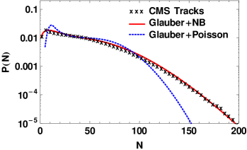
We use the multiplicity distributions of tracks observed in the minimum-bias p-Pb collisions cmswiki . In the three stage model of particle production, multiplicity fluctuations come from the fluctuations of the initial entropy of the fireball, from the entropy production during the viscous hydrodynamic stage, and from the statistical emission of hadrons at freeze-out. To a good approximation, in the considered regime of centralities the entropy after the hydrodynamic expansion is directly proportional to the initial entropy, which reflects the fact that the deterministic hydrodynamic evolution does not introduce fluctuations Olszewski:2013qwa . For independent statistical emission, the number of emitted hadrons is proportional to the final entropy and follows the Poisson distribution Kisiel:2005hn ; *Chojnacki:2011hb.

First, we consider the case where there is no weight distribution overlaid over the participant nucleons. Then the initial entropy is proportional to the number of participant nucleons and the distribution of the observed tracks is a convolution of three distributions: the distribution of participant nucleons, a Poisson distribution for each participant with a mean $\lambda$ defined as the average number of particles produced per participant, and a binomial distribution with success rate $p$ giving the probability of recording a track in the CMS acceptance. The folding yields the multiplicity distribution of the produced hadrons of the form

$$P(n)=\sum_{i}P_{part}(i)\frac{\left(\lambda pi\right)^{n}e^{-\lambda pi}}{n!},$$ (7)

where $P_{part}(i)$ is the distribution of the participant nucleons from the Glauber Monte Carlo. The parameter $\lambda p=5.36$ is chosen to reproduce the mean number of the observed tracks. As we can see (the dotted line in Fig. 3), the multiplicity distribution from the Glauber model convoluted with the Poisson distribution is much too narrow and does not reproduce the experimentally observed high-multiplicity tail.

The above shows that inserting a distribution of weights over the participant nucleons is necessary. In that case the distribution of the observed tracks is a convolution of four distributions: the distribution of participant nucleons, an overlaid distribution of weights, a Poisson distribution for the production of hadrons, and a binomial distribution for the experimental acceptance. When we use the distribution of weight in the form of the $\Gamma$ distribution (1), then its folding with the Poisson distribution yields the negative-binomial distribution (6), which we now take for hadrons produced per participant nucleon. One finds

$$P(n)=\sum_{i}P_{part}(i)N_{p\lambda i,\kappa i}(n).$$ (8)

The experimental multiplicity distribution is now very well reproduced with the parameter values $\lambda p=5.36$ and $\kappa=0.9$ (solid line in Fig. 3). We refer to this calculation as Glauber+NB.

The procedure outlined above is clearly a simplified picture of the multiplicity fluctuations in the relativistic nuclear collision. Further effects could be important, in particular the shape of the multiplicity distribution can depend on the pseudorapidity window, the track acceptance of the CMS detector is not uniform, particles from jets that contribute to the the tails of the multiplicity distribution do not increase the fluctuations in the thermalized fireball, or the entropy production in viscous hydrodynamics is not exactly linear. Nevertheless, the considered mechanism of additional density fluctuations in the fireball can serve as a model to illustrate its expected effects on the eccentricities and the harmonic flow coefficients. Such effects in A-A collisions have been considered previously in the Glauber scheme Broniowski:2007ft ; Rybczynski:2008zg and found to be relevant.

Figure 4: (Color online) A sample event evolution, visualized via the freeze-out isotherms in the $x-\tau$ plane (solid) and the $y-\tau$ plane (dashed). The standard case.

Figure 5: (Color online) Same as Fig. 4 for the compact-source case.

II.6 Hydrodynamics

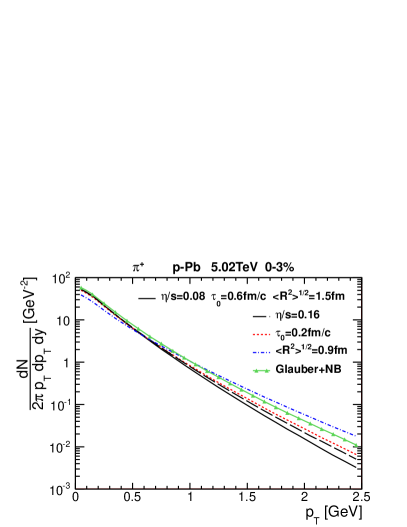
The hydrodynamic model used in this work is described in detail in Bozek:2011if . It carries out an event-by-event 3+1 D evolution and includes the shear and bulk viscosities. The multiplicity expected in central p-Pb collisions is extrapolated linearly in the number of the participating nucleons from the minimum bias results of the ALICE collaboration ALICE:2012xs . That way the average initial entropy per participant is adjusted. The shape of the entropy distribution follows the distribution of sources described in the previous section. The starting time of hydrodynamics is chosen to be $\tau_{0}=0.6$ fm/c for the standard case, but the evolution with the choice $\tau_{0}=0.2$ fm/c is also studied. The relatively short total duration of the collective expansion phase makes the results more sensitive to this very early stage and, possibly, to some nonequilibrium transient behavior Heller:2011ju ; *Berges:2013eia; *Florkowski:2013sk. The ratio of the shear viscosity $\eta$ to entropy density $s$ is $\eta/s=0.08$ or $\eta/s=0.16$, while the ratio of the bulk viscosity $\zeta$ to $s$ in the hadronic phase is $\zeta/s=0.04$ Bozek:2009dw . For each case (standard, compact, higher viscosity, lower initial time, or Glauber+NB) we produce initial configurations that are evolved event-by-event with hydrodynamics to obtain freeze-out hypersurfaces of the constant temperature $T_{f}=150$ MeV.

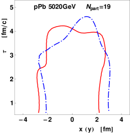
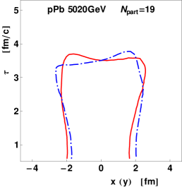
Two typical evolution histories for the standard and compact case, both for $N_{\rm part}=19$, are depicted in Figs. 4-5, where we show isotherms at $T_{f}=150$ MeV in the $x-\tau$ plane (solid lines) and in the $y-\tau$ plane (dashed lines). We note that although the systems originally have different sizes, the spatial spread of the isotherms at later times is similar, about 5 fm. The evolution of the standard source is about 15% longer than from the compact-source case. The radial flow is larger for the compact case, as the system is more squeezed initially. This leads to 20% higher values of the average transverse momentum.

.

Figure 6: (Color online) The model predictions for the mid-rapidity transverse momentum spectra of $\pi^{+}$ for the most central events. The solid line is for the standard calculation, with the initial source rms size of $1.54$ fm, $\eta/s=0.08$, and the initial time $\tau_{0}=0.6$ fm/c. The dotted line shows the results for the initial time of $0.2$ fm/c (and the other parameters unchanged), the dashed line stands for the calculations with $\eta/s=0.16$, and the dash-dotted line represents the calculation with the initial rms size $0.93$ fm/c. The solid line with the triangle symbols shows the Glauber+NB results, the case where the Glauber Monte Carlo initial conditions are convoluted with the $\Gamma$ distribution (cf. Sec. II.5).

The transverse momentum spectra depend on the choice of initial conditions. The $p_{T}$-spectra for $\pi^{+}$ are shown in Fig. 6. We notice that the spectra get harder with the increase of the shear viscosity, the decrease of the initial time $\tau_{0}$, or in the Glauber+NB case. The hardening of the spectra is most pronounced when starting the calculation from the compact source, which involves larger gradients present in the system.

II.7 Statistical hadronization

For each freeze-out configuration we generate 1000 THERMINATOR events to efficiently improve the statistics. This is a technical point, as physically one event should hadronize into one set of hadron distribution. The trick of running multiple THERMINATOR simulations on the same hydro event allows us to efficiently improve the statistics, as the computing time for the hydro evolution is two orders of magnitude longer than for the generation of a single THERMINATOR event.

We note that the statistical hadronization built in THERMINATOR contains the non-flow correlations from all resonance decays. The use of a full Monte Carlo generator of hadron distributions is also of practical merits, as it allows implementation of the kinematic cuts, acceptance or efficiency from the experimental setup, which is crucial in comparisons to the data.

II.8 Local charge conservation

Sizable correlations among opposite-charge particles result from the local charge conservation Bass:2000az . There are indications that this effect is generated at hadronization Jeon:2001ue ; *Bozek:2003qi; *Aggarwal:2010ya; Bozek:2012en , i.e., at the late stage of the reaction. Our implementation of the charge balancing is based on the assumption that the particle-antiparticle pairs of charged hadrons are emitted locally at freeze-out, carrying thermal distribution. The mechanism is described in detail in Ref. Bozek:2012en .

II.9 Transverse-momentum conservation

In our studies of the correlation variables we enforce the global transverse momentum conservation, which is important in correlation analyses Borghini:2000cm ; *Bzdak:2010fd. In particular, it affects the shape of the two-particle correlations in relative pseudorapidity and azimuth. To satisfy the constraint approximately we require the following condition on the global transverse momentum:

$$\sqrt{\left(\sum_{i}p_{x}\right)^{2}+\left(\sum_{i}p_{y}\right)^{2}}<P_{T},$$ (9)

where $i$ labels particles in the event. We have found numerically that in the central p-Pb system it suffices to take $P_{T}=5-10$ GeV. That way we retain 5-10% of the least-$P_{T}$ events from our full sample. A further lowering of $P_{T}$ does not affect the correlation results, while it deteriorates the statistics. The momentum conservation is imposed when calculating the di-hadron correlation functions. For the calculation of the elliptic and triangular flow, imposing the momentum conservation in that form is irrelevant.

II.10 Centrality definition

The simplest determination of the centrality classes in our model can be obtained from conditions on the number of the participant nucleons. The collisions with $N_{part}\geq 18$ amount to $3.4\%$ of the most central events from GLISSANDO. The next most central class is defined as $16\leq N_{part}\leq 17$, which forms centrality $3.4-7.8\%$. On the other hand, as noted in Bozek:2011if , simplistic centrality definitions based on the impact parameter are ill defined for central p-Pb collisions.

For the Glauber+NB case we define the centrality classes not by the number of participant nucleons, but through the total initial entropy in the fireball, i.e., we take into account the fluctuations from the overlaid $\Gamma$ distribution. A more accurate determination, following closely to the experimental setup, should impose the cuts on the final multiplicity of the produced particles, instead of on $N_{part}$ or the initial entropy.

III Two-particle correlations

III.1 Definitions

The basic objects of the study of this section are the two-dimensional two-particle correlation functions in relative pseudorapidity and azimuth. These quantities in comparison to the CMS data CMS:2012qk have already been analyzed in Bozek:2012gr . Here we extend this analysis, comparing to the ATLAS data ATLAS:pPb as well.

The simplest definition of the correlation function in the considered kinematic variables is

$$C(\Delta\eta,\Delta\phi)\equiv\frac{\langle\frac{d^{2}N^{\rm{pair}}}{d\Delta\eta\,d\Delta\phi}\rangle_{\rm events}}{\langle\frac{d^{2}N^{\rm{pair}}}{d\Delta\eta\,d\Delta\phi}\rangle_{\rm mixed\ events}}.$$ (10)

If the correlations were absent, $C_{(}\Delta\eta,\Delta\phi)=1$, thus unity is a natural scale for this measure. This correlation is used by the ATLAS collaboration ATLAS:pPb .

The “per trigger” correlation function, used by the CMS collaboration, is defined as CMS:2012qk

$$C_{\rm trig}(\Delta\eta,\Delta\phi)\equiv\frac{1}{N}\frac{d^{2}N^{\rm{pair}}}{d\Delta\eta\,d\Delta\phi}=B(0,0)\frac{S(\Delta\eta,\Delta\phi)}{B(\Delta\eta,\Delta\phi)},$$

with $\Delta\eta$ and $\Delta\phi$ denoting the relative pseudorapidity and azimuth of the particles in the pair. The signal and the mixed-event background are defined with the pairs from the same event, and the pairs from the mixed events, respectively:

$$S(\Delta\eta,\Delta\phi)=\langle\frac{1}{N}\frac{d^{2}N^{\rm{pair}}}{d\Delta\eta\,d\Delta\phi}\rangle_{\rm events},$$ (12)

$$B(\Delta\eta,\Delta\phi)=\langle\frac{1}{N}\frac{d^{2}N^{\rm{pair}}}{d\Delta\eta\,d\Delta\phi}\rangle_{\rm mixed\ events}.$$

The number of particles $N$ in the prefactor (denoted by CMS as $N_{\rm{trig}}$) is the number of charged particles in a given centrality class and acceptance bin, corrected for the detector efficiency. The multiplication with the central bin content $B(0,0)$ in Eq. (III.1) brings in the interpretation of Eq. (III.1) as the average number of correlated pairs per trigger particle.

To make quantitative comparisons easier, one also uses the projected correlation functions. A function used by the ATLAS collaboration is defined as

$$Y(\Delta\phi)=\frac{\int B(\Delta\phi)d(\Delta\phi)}{\pi N}C(\Delta\phi)-b_{\rm ZYAM},$$ (13)

where $S(\Delta\phi)$ and $B(\Delta\phi)$ are averages of $S(\Delta\eta,\Delta\phi)$ and $B(\Delta\eta,\Delta\phi)$ over the chosen range in $\Delta\eta$ avoiding the central region, in particular $2<|\Delta\eta|<5$ in the ATLAS analysis, and the constant $b_{\rm ZYAM}$ is such that the minimum of $Y(\Delta\phi)$ is at zero.

III.2 Comparison to the ATLAS data

Figure 7: (Color online) The charge-independent correlation function $C(\Delta\eta,\Delta\phi)$. The total transverse momentum is approximately conserved with the condition $P_{T}<10$ GeV. Charge balancing is included.

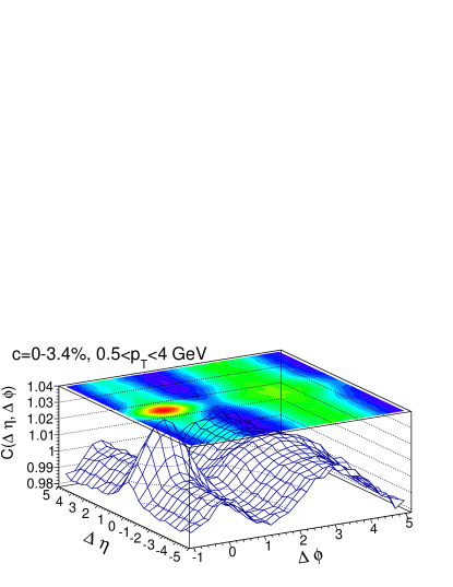
The result of our simulations for the most central p-Pb collisions ($c=0-3.4$ %) with the kinematic cuts corresponding to the ATLAS setup ATLAS:pPb is shown in Fig. 7. We display the standard-source case, as for the compact or Glauber+NB cases the results are quantitatively similar. We note the two prominent ridges, generated with flow, as well as the central peak, coming in our simulation from the charge balancing Bozek:2012en .

The same-side ridge appears naturally as a consequence of the collective flow. More precisely, in our framework the shape and flow in the fireball in the forward and backward rapidity regions is correlated, reflecting the assumption on the factorization of the transverse and longitudinal distributions in the initial condition. In particular, the principal axes of the elliptic flow are correlated along the whole pseudorapidity span. Thus, there are more pairs with $\Delta\phi\sim 0$ and $\Delta\phi~{}\sim\pi$ regardless of $\Delta\eta$. This “flow explanation” of the ridge formation is appealing in its simplicity.

Figure 8: (Color online) Projected and ZYAM-subtracted correlation function $Y\Delta(\phi)$ for the most central p-Pb collisions for the standard source (solid line) and compact source (dashed line), compared to the ATLAS data (points) at $\Sigma E_{T}^{Pb}>80$ GeV. The total transverse momentum is approximately conserved with the condition $P_{T}<5$ GeV. Charge balancing is imposed.

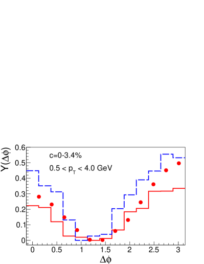
Next, to compare quantitatively to the data, we look at the projected correlation function $Y(\Delta\phi)$. There is a technical issue which must be discussed. By construction, the prefactor of $Y(\Delta\phi)$ is proportional to $\langle N(N-1)\rangle/\langle N\rangle$ – the ratio of the average number of pairs to the average number of particles. Thus to reproduce $Y(\Delta\phi)$ in a model calculation one needs to have proper correlations, but also correct fluctuations of the multiplicity. The second requirement is not easy to accomplish, in particular as ATLAS is using the transverse energy to define the centrality classes, and the fluctuations of multiplicity are large. For that reason in our comparison we rescale our model $Y(\Delta\phi)$ in such a way that the subtraction constant $b_{\rm ZYAM}$ is the same in the model and in the experiment. This assumes that the mechanism generating the flow and the ridge structures is “factorisable” from the multiplicity fluctuations.

The result of this procedure is shown in Fig. 8 for the most central collisions. We note that experimental data fall within our model results for the standard (solid line) and compact (dashed line) sources. We note that the compact source, leading to larger flow, has more prominent ridges.

The CMS correlation data for the p-Pb collisions have been compared to in our previous short paper Bozek:2013df , hence we do not repeat these results here, but only mention they are in semiquantitative agreement with the data.

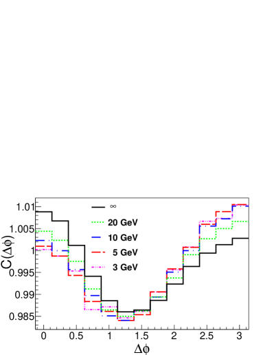
III.3 Effects of transverse momentum conservation

We can now demonstrate the relevance of the transverse momentum conservation and the simple procedure introduced in Sec. II.9. We use the projected correlation function $C(\Delta\phi)$ for that purpose. We note that limiting the value of the maximum total transverse momentum $P_{T}$ in the accepted events moves the strength from the same-side ridge to the away-side ridge. This is natural, as the momentum conservation increases the back-to-back motion of the particle. We note that for a practical purpose it is enough to use $P_{T}<5-10$ GeV. A further reduction changes the results very little at the expense of deteriorating the statistics. The numerical results, displaying the mentioned convergence, are shown in Fig. 9.

Figure 9: (Color online) Projected correlation function $C\Delta(\phi)$ for the most central p-Pb collisions for the standard source and several values of the maximum total transverse momentum $P_{T}$, listed in the legend.

IV Harmonic flow

IV.1 Cumulant method

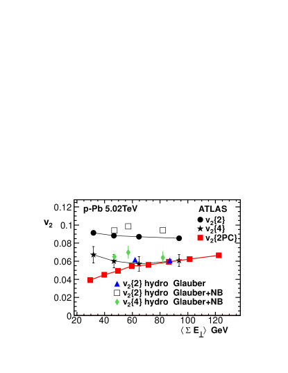
¿From the two- and four-particle cumulant method Borghini:2000sa ; *Bilandzic:2010jr we obtain the values of the flow coefficients collected in Table 2. The kinematic cuts correspond to the ATLAS experimental setup. We compare the standard and the Glauber+NB simulation, without or with the local charge conservation, and list the results for the two highest centrality classes. In Table 3 we show the dependence of $v_{2}\{2\}$ for the most central events on the parameters of the model: the value of the sheer viscosity $\eta$ and the time when hydrodynamics is initiated, $\tau_{0}$.

Table 2: Model predictions for the elliptic and triangular flow coefficients from the cumulant method for the p-Pb collisions at $\sqrt{s_{NN}}=5.02$ TeV. The cuts $|\eta|<2.5$, $0.3<p_{T}<5$ GeV correspond to the ATLAS setup. The standard and Glauber+NB cases are used, with $\eta/s=0.08$ and $\tau_{0}=0.6$ fm/c, without and with charge balancing. The errors are statistical and reflect the accumulated number of simulated THERMINATOR events (the actual error are somewhat larger due to a small number of the event sample).

	$c$=0-3.4%	$c$=3.4-7.8%
standard, no balancing
$v_{2}\{2\}^{2}$ [$10^{-3}$]	3.70(1)	3.78(2)
$v_{3}\{2\}^{2}$ [$10^{-3}$]	1.04(1)	0.95(1)
$v_{2}\{4\}^{4}$ [$10^{-6}$]	-0.4(4)	1.83(5)
$v_{3}\{4\}^{4}$ [$10^{-6}$]	0.0(2)	-0.3(3)
Glauber+NB, no balancing
$v_{2}\{2\}^{2}$ [$10^{-3}$]	8.18(12)	8.24(10)
$v_{3}\{2\}^{2}$ [$10^{-3}$]	1.52(8)	1.51(6)
$v_{2}\{4\}^{4}$ [$10^{-6}$]	15(7)	16(6)
$v_{3}\{4\}^{4}$ [$10^{-6}$]	-2(2)	-2(2)
Glauber+NB, with balancing
$v_{2}\{2\}^{2}$ [$10^{-3}$]	8.22(7)	8.68(6)
$v_{3}\{2\}^{2}$ [$10^{-3}$]	1.57(4)	1.62(4)
$v_{2}\{4\}^{4}$ [$10^{-6}$]	19(4)	19(4)
$v_{3}\{4\}^{4}$ [$10^{-6}$]	-1(1)	0(1)

Table 3: Parameter dependence of the predictions for the elliptic and triangular flow coefficient from the two-particle cumulant method for the p-Pb collisions at $\sqrt{s_{NN}}=5.02$ TeV, $c=0-3.4$ %, $|\eta|<2.5$, $0.3<p_{T}<5$ GeV. Charge balancing not included.

	$v_{2}\{2\}$ [%]	$v_{3}\{2\}$ [%]
standard
$\eta/s=0.08$, $\tau_{0}=0.6$ fm/c	6.09(1)	3.22(2)
$\eta/s=0.08$, $\tau_{0}=0.2$ fm/c	7.44(1)	4.49(1)
$\eta/s=0.16$, $\tau_{0}=0.6$ fm/c	5.57(1)	2.67(2)
$\eta/s=0.16$, $\tau_{0}=0.2$ fm/c	7.12(2)	4.01(2)
Glauber+NB
$\eta/s=0.08$, $\tau_{0}=0.6$ fm/c	9.0(1)	3.9(2)

We note several qualitative features from Tables 2 and 3:

• The dependence on centrality is very weak, as expected from the flow generated mainly by the fluctuations of the initial condition.

• The $v_{n}\{4\}^{4}$ coefficients are, within the statistical limit of our simulations, compatible with zero for the standard case, while for the Glauber+NB simulations $v_{2}\{4\}^{4}$ is positive. This again shows the fluctuation nature of the generated flow from the Glauber initial conditions. Additional fluctuations of the entropy deposited initially in the fireball increase the eccentricity and yield a nonzero value of $v_{2}\{4\}$ (cf. Table 1).

• Increased sheer viscosity quenches, as expected, the flow. The relative effect is stronger for higher harmonics.

• A shorter time of starting hydrodynamics increases the flow, which again is expected.

• The effect of the local charge balancing increases somewhat the flow coefficients.

As a matter of fact, the first two items above are crucial for the proper interpretation of the observed phenomenon. Detailed comparisons of the model predictions to experimental measurements provide a way of learning about the shape and fluctuations of the initial density in the p-Pb system. The observation of nonzero $v_{2}\{4\}$ by the ATLAS Collaboration Aad:2013fja indicates that in the small interaction region formed in the p-Pb collisions the large fluctuations of the energy deposited in each NN collision, as present in the Glauber+NB case, are crucial. Thus the initial conditions from the Glauber model in p-Pb collisions are fluctuation-dominated, analogously to the central A-A collisions. The same observation applies to the final elliptic and triangular flow in p-Pb collisions.

Figure 10: (Color online) The flow coefficients $v_{2}(\Delta\eta)$ (upper lines) and $v_{3}(\Delta\eta)$ (lower lines) calculated from the two-particle correlations as function of the relative pseudorapidity of the particles in the pair. The solid and dashed lines are for the unlike- and like-sign pairs, respectively. The central peak is due to charge balancing and, to a lesser extent, resonance decays.

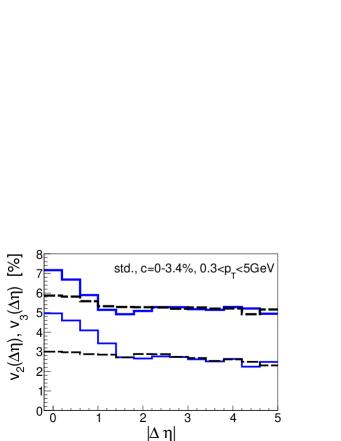
In view of the recent experimental results for the 2D correlations functions in p-Pb collisions, it is interesting to look at the possibility of measuring directly the harmonic flow coefficients. We plot the elliptic and triangular flow coefficients as functions of the pseudorapidity gap in Fig. 10. The quantities are obtained in our hydrodynamic model from the Fourier decomposition of the correlation function $C_{\rm trig}(\Delta\eta,\Delta\phi)$ Bozek:2012en . The non-flow effects present in our model are important only for pairs of small pseudorapidity separation. In the intervals $|\Delta\eta|>2$ the non-flow effects from the resonance decays and the local charge conservation can be neglected. We note that the flow coefficients in Fig. 10 are sizable, thus could be measured. It must be noted, however, that other sources of non-flow correlations may be present also in that kinematic region, but with smaller amplitudes, as measured in the p-p collisions Khachatryan:2010gv .

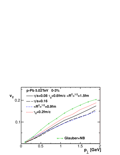
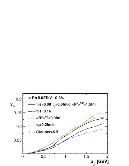
The $p_{\perp}$-dependent elliptic and triangular flow coefficients calculated with the two-particle cumulant method Borghini:2000sa are presented in Figs. 11 and 12. In the $p_{\perp}<2$ GeV range, where hydrodynamics applies, the flow coefficients show a typical hydrodynamic behavior and the magnitude of the flow is large. We find the elliptic (triangular) flow of about 10% (5%) for $p_{\perp}\sim 1$ GeV. The results are sensitive to the physical parameters of the model (cf. Table 3). The flow decreases for larger viscosity or when using compact initial conditions, and increases when starting the hydrodynamic evolution earlier. It also increases with the presence of additional initial fluctuations, as in the Glauber+NB case. We notice a larger relative variation for the triangular flow than for the elliptic flow when varying the parameters.

Figure 11: (Color online) The $p_{\perp}$ dependence of the elliptic flow coefficient of charged particles with $|\eta|<1$, obtained from the second-order cumulant method. The solid line corresponds to the standard calculation, $\eta/s=0.08$, $\tau_{0}=0.6$ fm/c, with the initial source rms size of $1.5$ fm, the dotted line shows the case where the initial time is reduced to $0.2$ fm/c, the dashed line stands for the calculations with increased viscosity, $\eta/s=0.16$, and the dash-dotted line represents the case of the compact source with rms size of $0.9$ fm/c. Finally, the solid line with the triangle symbols shows the Glauber+NB case (Sect. II.5).

Figure 12: (Color online) Same as Fig. 11 for the triangular flow coefficient, $v_{3}\{2\}$.

Figure 13: (Color online) The elliptic flow coefficient of charged particles for $|\eta|<2.5$, $0.3<p_{\perp}<5.0$ GeV from the cumulant method $v_{2}\{2\}$ and $v_{2}\{4\}$, and from the di-hadron correlation function measured by the ATLAS Collaboration Aad:2013fja , compared to our hydrodynamic calculation for the standard case ($v_{2}\{2\}$ at centralities 0-3.4% and 3.4-7.8%) and for the Glauber+NB case ($v_{2}\{2\}$ and $v_{2}\{4\}$ at centralities 0-5%, 5-10% and 10-20%). The corresponding transverse-energy for the centralities in the model calculations is obtained via interpolation of the experimental values.

IV.2 Scalar product method

The correlation between particles produced in p-Pb collisions can have different origin. A way to reduce some of the non-flow contributions to the harmonic flow coefficients is to use methods involving a rapidity gap between the reference particles defining the event plane orientation and the particles used to calculate the flow coefficient. In this subsection we present results for the scalar product method Adler:2002pu ; Luzum:2012da . One defines the $Q_{n}$ vector

$$Q_{n}^{A,B}e^{i\Psi_{n}}=\sum_{k}w_{k}e^{in\phi_{k}}$$ (14)

as a sum over charged particles in a given reference bin ($A$ or $B$). We use two definitions of the event plane, one with charged particles with $0.3<p_{\perp}<3$ GeV and $2.0<\eta<2.5$ (Pb side), or with $-2.5<\eta<2.0$ (proton side). The weights are equal to the transverse energy ($w_{k}=E_{\perp}$) for the $3.2<|\eta|<4.8$ bin. The resolution correction is

$$\bar{Q}_{n}^{A}=\sqrt{\frac{\langle Q_{n}^{A}Q_{n}^{B}\rangle\langle Q_{n}^{A}Q_{n}^{C}\rangle}{\langle Q_{n}^{C}Q_{n}^{B}\rangle}},$$ (15)

where the reference bin $C$ is defined in all cases as $0.3<p_{\perp}<3$ GeV and $|\eta|<0.5$. We have checked that the results do not differ noticeably when changing the $p_{\perp}$ or $\eta$ limits defining the $Q$ vectors. The flow coefficients are then calculated as

$$v_{n}^{A,B}\{SP\}=\frac{<Q_{N}^{A,B}\cos\left(n(\phi_{k}-\Psi_{n})\right)>}{\bar{Q}_{n}^{A,B}}.$$ (16)

The flow coefficients with reduced statistical error can be obtained with combined event planes on the proton and Pb sides.

Figure 14: (Color online) The elliptic (solid symbols and dashed line) and triangular (open symbols and solid line) flow coefficients obtained with the scalar product method. The circles and squares represent the calculation using the Q vector calculated on the proton and lead side, respectively. The lines show the result of combining the the two event planes.

Figure 15: (Color online) Comparison of the elliptic flow coefficients for $|\eta|<1$ calculated from the second cumulant method (solid line), from the scalar product method with event planes defined by charged particles in $2<|\eta|<2.5$ and $0.3<p_{\perp}<3.0$ GeV (dotted line), and from the scalar product method with event planes defined by the transverse energy in $3.2<|\eta|<4.8$ (dashed line).

Figure 16: (Color online) Same as Fig. 15 for the triangular flow.

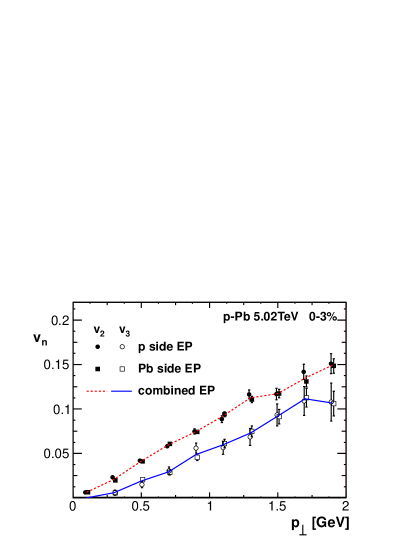
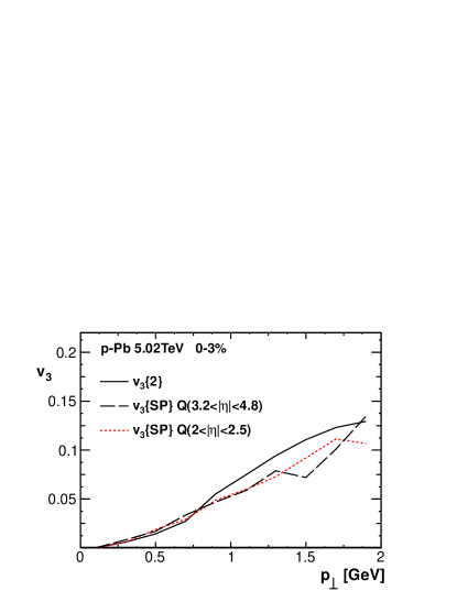
In Fig. 14 we show the elliptic and triangular flow coefficients obtained from the scalar-product method with the $Q$ vector from the bin $2.0<|\eta|<2.5$ on either the proton or the lead side. We notice that the two results are very consistent, with slightly smaller statistical errors for the $Q$ vector defined on the lead side. This reflects a better resolution of the event plane in that case. The azimuthally asymmetric initial source for hydrodynamic evolution is longitudinally extended, which yields a strong correlation between the event planes on the lead and proton sides. The observed two-particle correlation functions are almost symmetric for $\Delta\eta>0$ and $\Delta\eta<0$, which shows that the correlations are similar on the proton and the lead side CMS:2012qk . The consistency of flow correlations defined with $Q$ vectors for positive and negative rapidities justifies the use of the combined $Q$ vector, which reduces the statistical error.

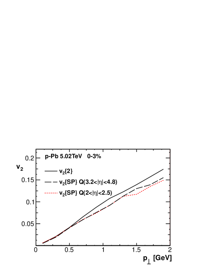
The results obtained with the $Q$ vectors defined by charged particle tracks or the calorimeter energy are compared to the results of the second cumulant method in Figs. 15 and 16. The elliptic and triangular flow coefficients obtained from the different definitions of the $Q$ vector are very similar. The second cumulant harmonic flow is calculated for smaller average pseudorapidity separation of the pair, thus contains some contribution of non-flow effects which increase the observed correlations. We expect that in the presence of additional non-flow correlation in the small system, such deviations could be larger. By comparing the second cumulant $v_{n}$ to methods using large rapidity gaps, the importance of such non-flow correlations could be estimated in the data.

IV.3 Correlations of flow and the initial geometry

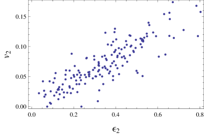
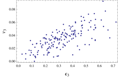
One of the main reasons to study the flow is to acquire the knowledge on the early phase of the reaction. One result that holds event-by-event is the proportionality of the eccentricity coefficients of the “geometric” distribution, $\epsilon_{n}$, to the coefficient of the harmonic flow of the produced hadrons, $v_{n}$. In Figs. 17 and 18 we show the event-by-event scattered plots of eccentricity-flow distributions. For this calculation the hydrodynamic events are combined from $1000$ THERMINATOR events corresponding to the same freeze-out configuration. We notice large correlation coefficients, defined as

$$\rho=\frac{\langle\epsilon_{n}v_{n}\{2\}\rangle-\langle\epsilon_{n}\rangle\langle v_{n}\{2\}\rangle}{{\rm var}(\epsilon_{n}){\rm var}(v_{n}\{2\})}$$ (17)

in these distributions, $\rho=0.85$ for the elliptic and $\rho=0.74$ for the triangular case, respectively. This feature, well know for the A-A collisions, is vividly present in our treatment of the p-Pb collisions.

Figure 17: The scattered plot of the event-by-event eccentricity-elliptic flow correlations. Glauber+NB, correlation coefficient 0.85.

Figure 18: Same as Fig. 17 for the triangular case. Correlation coefficient 0.74.

V Conclusion

We have analyzed various aspects of soft collective dynamics of the relativistic p-Pb collisions in the approach consisting of three stages: Glauber modeling of the initial phase, event-by-event viscous 3+1 D hydrodynamic, and statistical hadronization. Our analysis shows that the collective dynamics may very well be present in the highest-centrality p-Pb system formed in ultra-relativistic heavy-ion collisions. The application of the three-stage model, where the shape fluctuations in the initial stage are carried over to the harmonic flow coefficients in the hadronic spectra, allows for a quantitative understanding of the data for $v_{2}$ and $v_{3}$, as well as to describe the ridge structures in the two-particle correlation functions. The issues connected to the femtoscopic variables in p-Pb collisions, which display considerable sensitivity to collectivity, have been presented elsewhere Bozek:2013df .

Thus, following the successful experience of describing the A-A collisions in the three-stage approach, we argue that the collective scheme provides a natural and conventional explanation of numerous aspects of the soft dynamics of the “small” p-Pb system.

In central p-Pb collisions, the initial shape eccentricity parameters $\epsilon_{n}$ are entirely due to fluctuations. These fluctuations are enhanced by the distribution of overlaid weights on the spatial distribution of the participant nucleons. We find it quite remarkable that the same distribution that explains the multiplicity distribution of the produced hadrons in minimum-bias collisions leads also to quantitative agreement for the values of the elliptic and triangular flow coefficients measured recently by the ATLAS collaboration Aad:2013fja . This agreement includes the elliptic flow coefficient obtained from the four-particle cumulants.

We argue that the lowest harmonic flow coefficient may be measured directly in the LHC p-Pb experiments, hence we compute them through various methods (cumulant, scalar-product, rapidity-gap). These predictions, as well as the femtoscopic radii Bozek:2013df , will hopefully be verified shortly in the upcoming experimental analyzes.