Carnegie Supernova Project: Observations of Type IIn supernovae

Abstract

Aims. The observational diversity displayed by various Type IIn supernovae (SNe IIn) is explored and quantified. In doing so, a more coherent picture ascribing the variety of observed SNe IIn types to particular progenitor scenarios is sought.

Methods. Carnegie Supernova Project (CSP) optical and near-infrared light curves and visual-wavelength spectroscopy of the Type IIn SNe 2005kj, 2006aa, 2006bo, 2006qq, and 2008fq are presented. Combined with previously published observations of the Type IIn SNe 2005ip and 2006jd, the full CSP sample is used to derive physical parameters that describe the nature of the interaction between the expanding SN ejecta and the circumstellar material (CSM).

Results. For each SN of our sample, we find counterparts, identifying objects similar to SNe 1994W (SN 2006bo), 1998S (SN 2008fq), and 1988Z (SN 2006qq). We present the unprecedented initial $u$-band plateau of SN 2006aa, and its peculiar late-time luminosity and temperature evolution. For each SN, mass-loss rates of 10${}^{-4}-$10^-2 $M_{\odot}$ yr^-1 are derived, assuming the CSM was formed by steady winds. Typically wind velocities of a few hundred km s^-1 are also computed.

Conclusions. The CSP SN IIn sample seems to be divided into subcategories rather than to have exhibited a continuum of observational properties. The wind and mass-loss parameters would favor a luminous blue variable progenitor scenario. However the assumptions made to derive those parameters strongly influence the results, and therefore, other progenitor channels behind SNe IIn cannot be excluded at this time.

1 Introduction

Schlegel (1990) was the first to introduce the narrow-line Type IIn supernova (SN IIn) subclass to accommodate objects like SN 1987F (Wegner & Swanson 1996) and SN 1988Z (Stathakis & Sadler 1991; Turatto et al. 1993), which exhibit prevalent narrow-emission features. Today, members of this SN subclass cover a broad range of observational properties; however, they share the commonality of early phase spectra containing narrow Balmer emission features placed over a blue continuum. The most prominent features (e.g. H$\alpha$) typically exhibit multiple components, which consist of narrow cores (full-width-at-half-maximum FWHM_n of tenths to hundreds of km s^-1) that are often situated on top of intermediate-velocity components (FWHM${}_{i}\sim 1000$ km s^-1) and broad bases (FWHM_b of a few thousand km s^-1).

The multicomponent emission features are powered through a combination of SN emission and circumstellar interaction (CSI) processes. CSI occurs when the SN blast-wave shocks circumstellar material (CSM) (e.g. Chugai & Danziger 1994; Fransson et al. 2002), which originates in prevalent winds and/or violent eruptions of the progenitors during their pre-SN evolutionary phase (Kudritzki & Puls 2000).

In general, one finds that a forward shock is generated and propagates through the pre-SN wind as the outward moving SN blast-wave shocks CSM, while a reverse shock forms and propagates back through the expanding SN ejecta. At the interface between the forward and reverse shocks, a cold dense shell (CDS) of gas forms and rapidly cools through collisional de-excitation processes. Within the shock region, high-energy radiation is produced, which subsequently ionizes the un-shocked pre-SN wind. As this gas recombines, narrow emission lines are produced that can span a wide range in ionization potential (e.g. Chevalier & Fransson 1994; Chugai & Danziger 1994; Smith et al. 2009a).

Within this general picture, the broad-line component is typically associated with SN emission, although one cannot rule out thermal broadening of the narrow core for an optically thick wind (Chugai 2001). The intermediate-component originates in gas emitting in the post-shock region. Strong CSI also generates X-ray and radio emission (e.g. Nymark et al. 2006; Dwarkadas & Gruszko 2012; Chandra et al. 2012) and may also have an important influence on producing the necessary conditions to form dust, which has been detected in a handful of SNe IIn (see e.g. Fox et al. 2011).

Over the last two decades, observations have led to the realization of a remarkable heterogeneity between the photometric and spectroscopic properties, which have been exhibited by various SNe IIn (e.g. Pastorello et al. 2002; Kiewe et al. 2012). Today, the SNe IIn class consists of objects that show a large range in peak luminosities. At the very bright end of the distribution are SN 2006gy-like objects (Smith et al. 2007), which can reach peak absolute magntiudes of $M_{R}\lesssim$ $-$21, while at the faint end are objects like SN 1994aj, which reach peak values of $M_{R}\gtrsim$ $-$17 mag (Benetti et al. 1998).

Some SNe IIn are observable in the optical for years past discovery (e.g. SN 1995N, Fransson et al. 2002), while others fade to obscurity within months (e.g SN 1994W, Sollerman et al. 1998). Moreover, objects discovered soon after explosion indicate rise times ranging from several days to tens of days (see Kiewe et al. 2012). Around peak brightness, a handful of SNe IIn show Gaussian-shaped light curves (e.g. SN 2006gy), whereas others like SN 1994W exhibit a plateau light-curve phase that is reminiscent of Type IIP SNe (Kankare et al. 2012; Mauerhan et al. 2012a). The evolution of SN IIn light curves post-maximum also shows a large degree of heterogeneity.

Close examination of SN IIn spectra not only reveals the presence of multicomponent emission features but also a variety of emission line profiles, ranging from symmetric to highly asymmetric. These line profile asymmetries are often observed to grow over time. For example, prevalent attenuation of the red wing of H$\alpha$ in the cases of SNe 2006jd (Stritzinger et al. 2012, , hereafter S12) and 2010jl (Smith et al. 2012) was observed to increase over the first six months from discovery. Depending on the nature of the SN-CSM interaction, this behavior could be linked to increasing absorption due to dust condensation or to the occultation of radiation by a thick photosphere and/or surrounding CSM (e.g. a thick disk).

CSI has also been observed to occur in hydrogen poor core collapse (CC) SNe, which interact with helium-rich CSM. The prototype of this phenomenon is the Type Ibn SN 2006jc (Pastorello et al. 2008). Furthermore, some thermonuclear explosions may occur in a hydrogen-rich environment, producing Type IIn-like SNe Ia. Examples of these events include SNe 2002ic (Hamuy et al. 2003), 2005gj (Aldering et al. 2006; Prieto et al. 2007), 2008J (Taddia et al. 2012) and PTF 11kx (Dilday et al. 2012).

Progenitor stars of SNe IIn must eject enough mass to enable efficient CSI. A luminous blue variable (LBV) star, which was identified in pre-SN explosion images, has been linked to the Type IIn SN 2005gl (Gal-Yam & Leonard 2009). More recently, SN 2009ip has also been linked to an LBV (Mauerhan et al. 2012b), which has exhibited episodic rebrightening events three years prior to core collapse. However, Pastorello et al. (2012) and Soker & Kashi (2012) have suggested that the last bright event of SN 2009ip is due to other mechanisms rather than to core-collapse. LBVs are known to suffer significant mass loss ($\dot{M}\sim 10^{-2}-10^{-3}\leavevmode\nobreak\ M_{\odot}\leavevmode\nobreak\ yr^{-1}$) through episodic outbursts that occur on time scales ranging from months to years. This behavior is well-documented through detailed observations of Eta Carinae and other “SN impostors” (e.g. see Smith et al. 2011).

Nevertheless, the variety of SN IIn properties suggests that their origins may lie within a diversity of progenitor stars. For example, Fransson et al. (2002) and Smith et al. (2009b) have suggested that red supergiant (RSG) stars, which experience a pre-SN mass-loss phase driven by a superwind, could be viable progenitors for a large fraction of observed SNe IIn. This behavior is observed in VY Canis Majoris.

A proper determination of the progenitor mass-loss history is crucial to discern the nature of the progenitor itself. Estimates of mass-loss rates found in the literature often assume that the progenitor wind is steady, even though X-ray observations demonstrate that this is likely not the case for the majority of objects (Dwarkadas 2011). Ad hoc assumptions on the density profiles of progenitor pre-SN winds can therefore lead to incorrect mass-loss rate estimates. From the theoretical point of view, steady, line-driven winds are the only mass-loss mechanism that is reasonably understood (but see Smith et al. 2011, and reference therein), whereas the physics behind episodic and eruptive mass loss behavior is still in its infancy (see e.g. Smith & Owocki 2006; Yoon & Cantiello 2010).

In this paper, we present and analyze optical and near-infrared (NIR) light curves and visual-wavelength spectroscopy of five SNe IIn observed by the Carnegie Supernova Project (CSP, Hamuy et al. 2006). These new objects are SNe 2005kj, 2006aa, 2006bo, 2006qq, and 2008fq. Basic information of these SNe IIn is provided in Tables 1 and 2. In addition to these five objects, the full CSP SN IIn sample includes detailed observations of SNe 2005ip and 2006jd, which are presented by S12.

The organization of this paper is as follows: Sect. 2 contains details concerning data acquisition and reduction; Sect. 3 describes the CSP SN IIn sample; Sect. 4 reports the broad-band optical and near-infrared photometry; Sect. 5 describes the spectroscopic observations; Sect. 6 presents the discussion and the interpretation of the data; and finally, Sect. 7 presents the conclusions.

2 Observations

Optical and NIR photometry of the five SNe IIn, which are presented in this paper, were computed from images obtained with the Henrietta Swope 1 m and the Irénée du Pont 2.5 m telescopes located at the Las Campanas Observatory (LCO). The vast majority of optical imaging were taken with the Swope, which was equipped with the direct imaging camera known as “Site3” and a set of Sloan $ugri$ and Johnson $BV$ filters. A small amount of optical imaging was also obtained for two objects, SNe 2006aa and 2006bo, using the du Pont, which was equipped with a direct imaging camera named after its chip Tek-5, also known as “Tek-cinco”. NIR imaging was performed with both the Swope ($+$ RetroCam) and du Pont ($+$ Wide Field IR Camera, WIRC), which were equipped with a set of $YJH$ filters. A small amount of $K_{s}$-band imaging was also obtained with the du Pont for SNe 2005kj and 2008fq. The Magellan (Baade) telescope at LCO was also used to get three epochs of $K_{s}$-band imaging for SN 2005kj. Complete details concerning the instruments and passbands used by the CSP can be found in Hamuy et al. (2006), Contreras et al. (2010) and Stritzinger et al. (2011).

A detailed description of CSP observing techniques and data reduction pipelines can be found in Hamuy et al. (2006) and Contreras et al. (2010). In short, each optical image undergoes a series of reduction steps consisting of (i) bias subtraction, (ii) flat-field correction, and (iii) the application of a shutter time and CCD linearity corrections. Given the nature of observing in the NIR, the basic reduction process for these images consists of (i) dark subtraction, (ii) flat-field correction, (iii) sky subtraction, (iv) non-linearity correction, and finally, (v) the geometrical alignment and combination of each dithered frame.

Deep template images of each SN host galaxy were obtained using the du Pont telescope under excellent seeing conditions. The templates are used to subtract away the host contamination at the position of the SN from each science image (see Contreras et al. 2010, for details). In Table 6, the UT date of each template observation is reported. In some cases (e.g. SNe 2005kj and 2006qq), we had to wait several years after discovery to obtain useful templates without SN contamination because of the long-lasting CSI and late-time dust emission. SNe 2005ip and 2006jd are still bright, and templates are not available (S12).

PSF photometry of each SN was computed differentially with respect to a local photometric sequence of stars. The calibration of the photometric sequences was done with respect to Smith et al. (2002) ($ugri$), Landolt (1992) ($BV$), and Persson et al. (1998) ($YJHK_{s}$) standard fields observed over a minimum of three photometric nights. The local sequences for each CSP SN IIn in the standard photometric systems are provided in Table 3, while final SN optical and NIR photometry in the natural system are listed in Table 4 and Table 5, respectively.

Visual-wavelength spectroscopy of the CSP SN IIn sample was obtained using the Du Pont and Magellan (Baade ad Clay) telescopes at LCO and the ESO New Technology Telescope (NTT) at the La Silla Observatory. A spectrum of SN 2005kj was obtained with the 60-inch telescope at the Cerro Tololo Inter-American Observatory (CTIO). These data were reduced in a standard manner as described by Hamuy et al. (2006), which included: (i) overscan correction, (ii) bias subtraction, (iii) flat-fielding, (iv) 1-D spectrum extraction, (v) wavelength calibration (vi) telluric corrections, (vii) flux calibration, and (viii) combination of multiple exposures. Finally, the flux of each spectrum was adjusted to match broad-band photometry. The journal of the spectroscopic observations is provided in Table 7.

3 The CSP SN IIn sample

Table 1 lists the properties of the full CSP SN IIn sample, which include the SN coordinates, its host galaxy name, type, distance, the estimates of total absorption [$E(B-V)_{MW}$ $+$ $E(B-V)_{host}$] and the equivalent width (EW) of interstellar Na i D absorption. Finding charts for the five new CSP SNe IIn are given in Fig. 1. As most of the SNe followed by the CSP were discovered by targeted surveys, it is not surprising that the hosts of the CSP SN IIn sample are bright, nearby spiral galaxies in the redshift range of 0.007$\leq$z$\leq$0.029. Quoted distances to each event correspond to the luminosity distances that are provided by NED, which include corrections for peculiar motion (GA+Shapley+Virgo) and are based on cosmological parameters obtained by WMAP5 (Komatsu et al. 2009). Galactic absorption values were taken from NED (Schlafly & Finkbeiner 2011), while estimates of $E(B-V)_{\rm host}$ were determined through the combination of EW measurements of interstellar Na i D absorption lines at the host-galaxy redshift and the relation $E(B-V)_{\rm host}=0.16\cdot\rm EW({\rm{Na\textsc{i}}\leavevmode\nobreak\ D})_{\rm h}$ (Turatto et al. 2003). Only two objects display significant Na i D absorption. SN 2006qq exhibits clear Na i D absorption at the host rest frame in the spectrum taken on January 1, 2007. We note that the host galaxy of this object is remarkably tilted, exhibiting an inclination between the line of sight and its polar axis of 85.6 deg. SN 2008fq, which is located close to the center of its host, shows prominent narrow absorption lines of Na i D in each spectrum, although the individual D1 and D2 components are not resolved. In the case of SN 2008fq, we take the mean of the EW measurements as obtained from our series of spectra. We determined $E(B-V)_{\rm host}$ $=$ 0.12 and 0.46 mag for SN 2006qq and 2008fq, respectively. We note, however, that the EW of Na i D from low resolution spectra is a debatable proxy for the extinction of extragalactic sources, and it does not work for SNe Ia (Poznanski et al. 2011).

Table 2 indicates that several of the objects were discovered within a few days to weeks past the last non-detection. Specifically for three SNe IIn, we have early observations and good constraints on their explosion epoch (see column 5 in Table 2). Only SNe 2005kj and 2006bo have poorly constrained explosion dates. As noted in S12, SNe 2005ip and 2006jd are believed to have been discovered soon after explosion. In what follows, the discovery date is used to define the temporal phase of each object.

Plotted in Fig. 2 are the optical and NIR light curves of the five new CSP SNe IIn. Typically, each SN was observed for approximately 100 days with a cadence of several days, however, the SN 2005kj observations extend to over 180 days. Due to scheduling constraints, the NIR coverage typically is with a lower cadence.

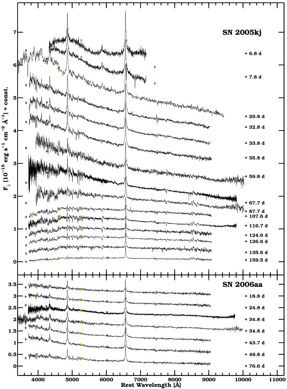
Figure 3: Spectroscopic sequences of SNe 2005kj and 2006aa. Days relative to the discovery epoch are reported next to each spectrum. Fluxes obtained from interpolated magnitudes at the epoch of each spectrum in each optical filter are marked by diamonds.

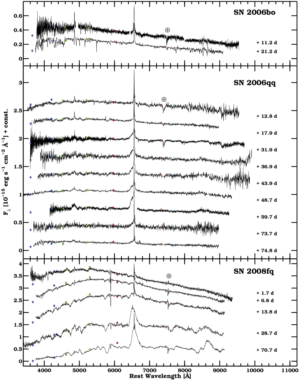
Figure 4: Spectroscopic sequences of SNe 2006bo, 2006qq and 2008fq. Days relative to the discovery epoch are reported next to each spectrum. Fluxes obtained from interpolated magnitudes at the epoch of each spectrum in each optical filter are marked by diamonds.

As indicated in Table 7 the number of optical spectra for this sample of five SNe IIn vary from two (SN 2006bo) to 15 (SN 2005kj) epochs. Spectroscopic follow-up started from a maximum of 19 days after discovery (i.e. SN 2006aa) down to a minimum of 2 days after discovery (i.e. SN 2008fq). Depending on the exact instrument used, the wavelength coverage typically ranges from 3800 Å to 9300 Å (see Table 7). The spectroscopic sequences of these five SNe IIn are presented in Fig. 3 and Fig. 4. Included in each panel as colored diamonds are photometric broad-band measurements derived from interpolated light curves.

Our dataset is also complemented with data published in the literature. Several of the SNe IIn in our sample were observed in the mid-infrared (MIR) with the Spitzer Space Telescope (Fox et al. 2011). In particular, late-phase Spitzer observations of SN 2006qq (approximately 1050 days past discovery) found this object to be quite bright at $\lambda>$3.6 $\mu$m, while similar imaging of SNe 2006aa and 2006bo showed no MIR emission.

4 Photometry

4.1 Light curves

SN 2005kj was observed only after maximum light, and its explosion date is not well constrained by pre-explosion images. Its optical light curves (Fig. 2) show a decline of approximately 3.5 mag in the first 100 days in the $u$ band, whereas the decline is slower for the redder bands in the same time interval ($i$ band becomes only 0.8 mag fainter). After 100 days the light curve slope steepens, the $i$ band decays by 1.4 mag in the following 70 days, and the bluer bands show a higher rate of decline. The NIR light curves exhibit a somewhat slower evolution at all phases. The SN was detected even at 382 days in $Y$ and $J$ bands (see Table 5).

SN 2006aa was discovered relatively young and has an uncertainty of $\pm$8 days on the explosion date. Its light curves are characterized by a “Gaussian” shape with an initial rise that culminates at maximum light approximately 50 days after discovery for all the filters. Interestingly, the super-luminous SNe II (Gal-Yam 2012) and the peculiar SN Ib/c 2005bf (Folatelli et al. 2006) peak at 50-60 days. However, no sign of interaction was seen in the case of SN 2005bf, and its long rise time can be attributed to the delay in the diffusion of photons through the ejecta. The rise in the $u$ band follows an initial 10 day “plateau”. This feature is observed for the first time in the SN IIn class for which a small number of early time observations in the near ultraviolet exists. We note that the SN IIn 2011ht did not present this “plateau”, although it was discovered soon after explosion (Roming et al. 2012). After maximum light, the light-curve decline is steeper in the bluer bands, as seen in SN 2005kj, with $B$ and $i$ bands fading by approximately 2 mag and 1 mag respectively in about 80 days.

SN 2006bo was discovered after maximum light (its explosion date is not well-constrained from pre-SN images), and its optical light curves are characterized by an initial linear decline (in mag), which is more pronounced in the bluer bands. In the first 40 days, the $u$ band faded by approximately 2 mag, whereas the $i$ band faded by only 0.5 mag. The last optical observation that was obtained approximately 150 days after discovery and 3 months subsequent to the previous optical observation reveals an increase in the decline rate some point after 60 days. The NIR light curves cover only the first tens of days after discovery and are nearly flat, showing only a marginal decline in brightness.

SN 2006qq was observed after its maximum light in the optical bands and before its maximum light in the NIR. Each optical band is characterized by a decline, which becomes progressively less steep with time and wavelength. The NIR light curves show a maximum emission at 20–30 days after discovery. The SN was detected in $H$ band later than 700 days after discovery (see Table 5).

SN 2008fq was discovered prior to 9 days after explosion. It has a light curve that exhibits a fast rise, which culminates in an early maximum (approximately 10 days in $B$ band, 20 days in $i$ band, and a few days later in the NIR). Then a steep decline lasts approximately 2 weeks, which is followed by a slow, linear decline until the end of the observations (approximately day 70).

We determined the slopes of the optical light curves by dividing the difference in magnitude of contiguous photometric epochs by their temporal difference and then fitting the obtained slopes with low-order polynomials. The slope evolutions confirm that bluer bands tend to decline faster than redder bands after maximum light (this is not true for the long-lasting SNe 2005ip, 2006jd, and for SN 2006qq). The decline after maximum light is not linear at least for those objects which were observed for less than 100 days, whereas SN 2006qq shows an almost linear decline in each band after 100 days. For SNe 2005kj and 2006aa, the decline rate increases with time; for SNe 2005ip, 2006jd and 2006bo, the decline rate decreases. When we compare the decay rate of ⁵⁶Co (0.0098 mag day^-1) with that of the $V$ band for the five SNe that are observed after 100 days since discovery, we find that only SN 2006qq (and marginally SN 2005ip) has a slope compatible with radioactive decay. SN 2006bo might also be characterized by a late-time decline rate, which is compatible with radioactive decay. Unfortunately, the data do not allow us to confirm it. Decay rates at 100 days are summarized in Table 8.

4.2 Absolute magnitudes and colors

Armed with the distances and $E(B-V)_{tot}$ color excess values listed in Table 1, absolute magnitude light curves were computed for the entire CSP SN IIn sample and were plotted in Fig. 5 (top panels). In doing so, a standard reddening law characterized by an $R_{V}$ $=$ 3.1 (Cardelli et al. 1989) was used to convert $E(B-V)_{tot}$ to absorption in each photometric bandpass. We assume that the host reddening is zero for the SNe with no detectable Na i D.

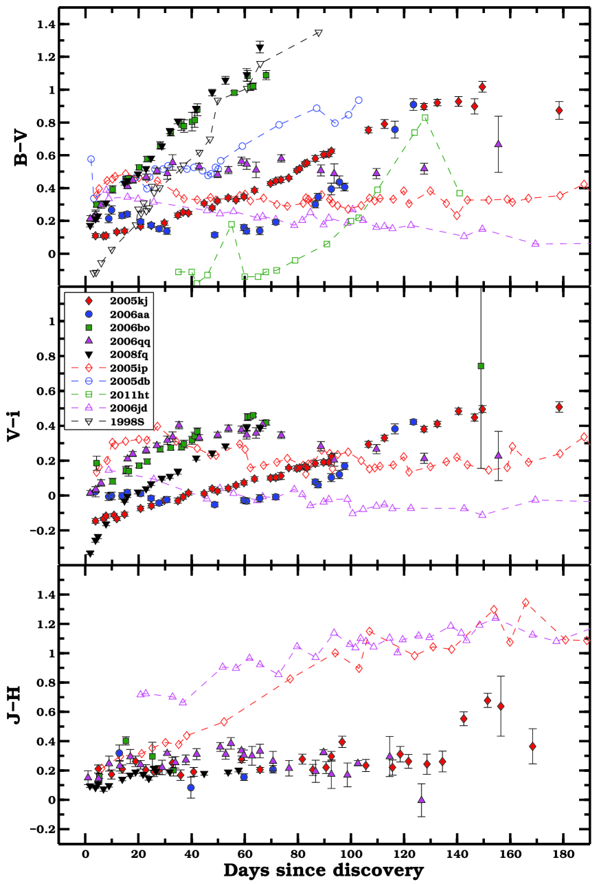
Figure 6: Intrinsic optical and NIR color-curve evolution of the CSP SNe IIn sample. The top panel $B-V$ color curves also include several objects from the literature (see caption of Fig. 5 for references).

Since it is approximately 1 mag more luminous than SNe 2005kj, 2006aa, and 2006qq, SN 2008fq turns out to be the intrinsically brightest object in the sample. We note that SN 2008fq was corrected for a substantial amount of extinction ($A_{V}$ $=$ 1.6 mag), which is derived from Na i D absorption that is known to provide poor constraints on reddening (Blondin et al. 2009; Folatelli et al. 2010; Poznanski et al. 2011). Nevertheless, when adopting the Na i D-based color excess, the $r$-band light curve of SN 2008fq reaches a maximum value only 0.2 mag brighter than that of SN 1998S (Liu et al. 2000), which exhibits similar light curve shape and spectral properties (see bottom panel of Fig. 5 and Sect. 5.6). With this color excess, the intrinsic broadband colors of SN 2008fq also appear consistent to those of SN 1998S, as revealed in the top panel of Fig. 6. Peaking at $V$ $=$ $-$19.3 mag, SN 2008fq belongs to the bright-end of the “normal” SN IIn category, whereas the super-luminous SNe IIn exhibit absolute magnitudes brighter than $-21$ (Gal-Yam 2012).

Since it is approximately 2 mag less luminous than SN 2008fq at peak and never brighter than $V$ $\approx-$17 mag, SN 2006bo is the faintest object within the full CSP SN IIn sample. The $r$-band light curve evolves along a plateau phase over the first two months of monitoring and, as revealed in Fig. 5, is similar in overall shape to the 1994W-like SN 2011ht (Mauerhan et al. 2012a) but with a somewhat fainter luminosity along the plateau. Since the explosion epoch of SN 2006bo is poorly constrained, it may have been discovered weeks after explosion. This possibility would then imply a higher tail luminosity as compared to that of SN 2011ht.

SNe 2005kj, 2006aa, and 2006qq have peak $V$- and $r$-band absolute magntiudes between $-$17.7 and $-$18.5 mag. Among them, SN 2006qq decays similarly to the slow-declining and long-lasting SNe 2005ip and 2006jd (S12), although it is brighter than those objects (see Fig. 5). In addition, SN 2005kj exhibits a relatively high luminosity for more than 180 days, but its decline rate beyond 100 days is larger than that of SN 2006qq. The evolution and brightness of the $r$-band light curve of SN 2006aa closely resembles that of SN 2005db (Kiewe et al. 2012). However, the rise time for SN 2006aa is particularly long (approximately 50 days). SN 2006aa also displays faint emission in the NIR, since it is approximately 1 mag fainter than the bright SN 2008fq.

Estimates of the peak absolute magnitudes, derived from the individual light curves of each SN, are given in Table 9. These values have been determined by fitting the light curves with low-order polynomials. For completeness, the peak absolute magnitudes of SNe 2005ip and 2006jd are also included in Table 9 (S12).

Figure 6 contains the comparison of intrinsic $B-V$, $V-i$, and $J-H$ colors of the full CSP SN IIn sample. For comparison, the panel containing the $B-V$ color curve evolution also includes several well-observed objects taken from the literature. Both the $B-V$ and $V-i$ color curves indicate that SNe IIn evolve to the red over time, and in this sample, SNe 2008fq and 2006bo show the largest $B-V$ color evolution ranging from 0.2 mag to 1.0 mag over a period of approximately 50 days. SN 2006bo appears to be much redder than the 1994W-like SN 2011ht, even though the light curve shapes are similar. SNe 2005kj and 2006qq experience a slow cooling, which is comparable to that of the long-lasting SNe IIn 2005ip and 2006jd. In particular, SN 2005kj takes approximately 120 days to reach a $B-V$ $=$ 1.0 mag. Interestingly, SN 2006aa first evolves to the blue, then reaches a minimum value in the optical colors at the time of maximum light, and then evolves to the red over time.

The NIR ($J-H$) color curves follow more flat trajectories compared to the optical color curves. However, the $J-H$ color curve clearly exhibits values that increase over time in the case of SNe 2005ip and 2006jd, and this evolution is likely driven by emission related to newly formed dust (Fox et al. 2011, S12).

4.3 Bolometric properties

The photometric dataset of our CSP SN IIn sample is well-suited to construct quasi-bolometric light curves. To do so requires the interpolation (or when necessary extrapolation) of NIR magnitudes at epochs that coincide with the optical observations. Next, broad-band magnitudes were converted to fluxes at the effective wavelength of each bandpass. After correcting each flux point for reddening, a spectral energy distribution (SED) at each observed epoch was fit with a spline, which resulted in a nearly complete UV-optical-NIR (UVOIR) SED. The SEDs were then integrated over wavelength space spanning from $u$ to $H$ band, and then the final UVOIR luminosity was computed by multiplying the UVOIR flux with 4$\pi$D${}_{L}^{2}$ (where D_L is the luminosity distance). The error on $L$ was obtained through simulating hundreds of SEDs (according to the uncertainties on the specific fluxes) and taking the standard deviation of their integrals.

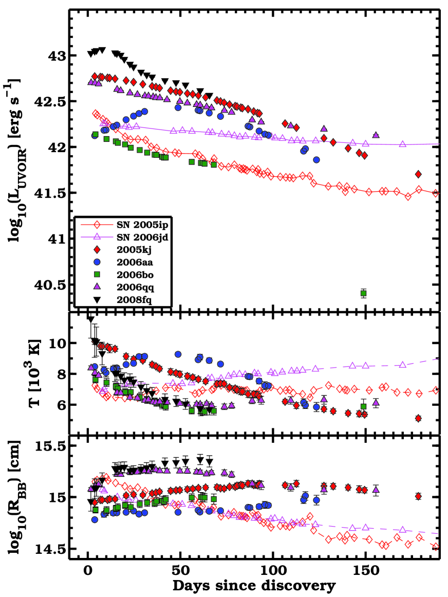
Figure 7: (Top panel) UVOIR light curves for the full CSP SN IIn sample. Theoretical light curve tails powered by radioactive decay for different amounts of ⁵⁶Ni are included as dashed lines. (Middle panel) Temperature evolution derived from BB fits to the time-series of SEDs. For SNe 2005ip and 2006jd we plot the temperature associated with the optical emission (see S12). (Bottom panel) Radius evolution was computed assuming BB emission. For SNe 2005ip and 2006jd, we plot the radius associated with the optical emission (see S12).

The final UVOIR light curves for the full CSP SN IIn sample are plotted in the top panel of Fig. 7. As observed in the $r$-band absolute magnitude light curves, SN 2008fq and SN 2006bo are the brightest and faintest objects within the CSP SN IIn sample, respectively, while SN 2006aa and SN 2008fq appear to have been discovered before reaching maximum. The peak bolometric luminosities range from those of normal CC SNe IIP to values 10 times higher, which are comparable to those of luminous SNe II (Inserra et al. 2012).

Inspection of the late phase portion of the UVOIR light curves reveals that the sample exhibits a diversity of decline rates, ranging from values both above and below the expeced decline rate of the full trapping of energy produced by the radioactive decay chain ⁵⁶Co $\rightarrow$ ⁵⁶Fe. SNe 2005kj and 2006aa exhibit steeper slopes than those expected for full trapping of gamma-rays that are produced from the ⁵⁶Co decay, while the slopes of SNe 2005ip, 2006jd, and 2006qq are more shallow. UVOIR light curve decline rates at 100 days after discovery are reported in Table 8. The inconsistency between observed and ⁵⁶Co decline rates suggests radioactivity is not the prevalent energy source for these objects.

The SEDs were also used to estimate temperature ($T$) and radius ($R$) of the emitting region, by using black-body (BB) fits. When performing the BB fits, $u$- and $B$-band flux points were excluded, because they sample portions of the optical spectrum that suffer a significant reduction in continuum flux because of line blocking effects, particularly at late epochs. In addition, the $r$ band was also excluded from the BB fits given the presence of prevalent H$\alpha$ emission.

The time evolution of $T$ and $R$ for the full CSP SN IIn sample is plotted in the bottom portion of Fig. 7. During early epochs, $T$ monotonically drops over time for each SN except for SN 2006aa, which shows a peak at approximately 9000 K at the time of maximum light. At epochs past 50 days after discovery, all objects decrease in $T$ except for SNe 2005ip and 2006jd, which both show enhanced thermal emission related to dust condensation (S12). The maximum $T$ values range from approximately 7000 to 11,500 K and decline over time to values no less than 5500 K by about day 60. These values are consistent with SNe IIn presented in the literature (see e.g. Smith et al. 2009a).

For all the SNe with a SED that is well fit by a single BB component (i.e. all objects, except SNe 2005ip and 2006jd), Fig. 7 also reveals that $R$ slowly increases over time until it reaches an almost constant value. Typical radii extend to approximately 10¹⁵ cm, which is also typical for many SNe IIn in the literature (e.g. SN 1998S, Fassia et al. 2001). In a SN IIn, most of the continuum emission is likely to come from an expanding thin cold-dense shell. This shell continually expands to larger radii. However, the black-body (BB) radius appears to stall or in some cases, even to shrink, because the shell-covering factor decreases as the optical depth drops. This was discussed by Smith et al. (2008), where they present SN 2006tf.

5 Spectroscopy

In this section, the visual-wavelength spectra of the five new CSP SNe IIn are analysed and compared to other objects in the literature. A special emphasis is placed on constraining the evolution of both luminosity and line profile shape for the H$\alpha$ and H$\beta$ emission features. We note that the resolution of our spectra (see Table 7) allow us to resolve H$\alpha$ FWHM velocities down to only 320 km s^-1 for SNe 2008fq, while H$\alpha$ FWHM velocities are resolved down to 180 km s^-1 for the other objects.

5.1 SN 2005kj

The spectral sequence of SN 2005kj (Fig. 3, top panel) covers approximately 150 days of evolution. Each spectrum exhibits prevalent, symmetric Balmer emission lines. The left panel of Fig. 8 displays the H$\alpha$ and H$\beta$ emission features, which were fit by multiple Lorentizian components, while the right panel contains the flux and velocity evolution of both features. Flux and velocity measurements are also reported in Tables 10 and 11.

During the first 70 days of evolution, H$\alpha$ and H$\beta$ are characterized by a narrow FWHM_n $\approx$ 1000 km s^-1 and a broad FWHM_b $\approx$ 2500 km s^-1 component. Around 70 days, the broad component becomes difficult to detect, while H$\beta$ begins to form a P-Cygni profile with an absorption minimum of $v_{min}$ $=-$600–800 km s^-1.

H$\beta$ is initially very bright and almost comparable to H$\alpha$ in luminosity. However, the Balmer decrement increases over time, and H$\beta$ is found to be much fainter at late epochs. The total flux of both H$\alpha$ and H$\beta$ drops over time. The H$\gamma$ and H$\delta$ lines are also detected: both exhibit a P-Cygni profile that shows a minimum absorption with similar velocity to H$\beta$. After approximately 35 days, they are barely discernible from the noise.

He i $\lambda$5876 is visible until $\approx$ 20 days, showing narrow and broad components in emission. Concerning the narrow absorption lines, Na i D is not detected during early epochs; however, the presence of Ca ii H&K $\lambda\lambda$3933,3968 is clear. Numerous Fe ii and Ti ii P-Cygni profiles are visible in the blue portion of the spectra of SN 2005kj from day $+$32.8. At epochs $\gtrsim$70 days, the Ca ii triplet and O i $\lambda$8447 emerge, and at later times ($\gtrsim$100 days), a P-Cygni profile identified with Na i D is also visible. The continuum flux, initially dominated by UV and blue photons, progressively becomes red, as expected from the decreasing temperature (see Fig. 7, middle panel).

5.2 SN 2006aa

The seven spectra that we obtained for SN 2006aa (Fig. 3, bottom panel) are typical SN IIn spectra, which are mainly characterized by Balmer emission lines (in particular H$\alpha$ and H$\beta$, but also H$\gamma$ and H$\delta$). As shown in Fig. 9, their continuum-subtracted, extinction-corrected profiles are well fit by the sum of a broad (FWHM${}_{\rm b}\approx$2000 km s^-1) and a narrow (FWHM${}_{\rm n}\lesssim$700 km s^-1) Lorentzian in emission. In addition, a narrow Lorentzian in absorption is fit at $\approx-$800 km s^-1 from the central wavelength, in order to reproduce the narrow absorption feature. The H$\alpha$ and H$\beta$ broad-component fluxes reach maximum values when the SN is at maximum light, whereas the narrow component exhibits nearly constant emission over time. Fluxes and velocities of the most important hydrogen lines are reported in Tables 12 and 13.

Fe ii features are observed in all the spectra (between 20 and 80 days). As in the case of SN 2005kj, narrow lines of Na i D in absorption are not detected at the host galaxy rest frame, whereas narrow Ca ii H&K absorption lines are observed. The spectral continuum is well fit by a BB function with temperature T_BB $=$ 8000-10000 K.

5.3 SN 2006bo

Only two early-time spectra were collected for SN 2006bo (Fig. 4, top panel). However, these reveal an interesting H$\alpha$ profile (see Fig. 10), which is characterized by a prevalent narrow emission (FWHM${}_{\rm n}\approx$1000 km s^-1) feature and an absorption component at $\approx-$600 km s^-1. Identical features are present in H$\beta$ and in the faint H$\gamma$ line, where the absorption is even more pronounced. This is a case of a SN IIn that shows no clear signatures of a broad component. H$\alpha$ and H$\beta$ fluxes and velocities are given in Tables 14 and 15.

No Na i D absorption features are found in the spectra at the redshift of SN 2006bo; however, features attributed to Ca ii H&K are discernible. Fe ii and Ti ii P-Cygni profiles are also observed, while weak traces of the Ca ii NIR triplet characterize the red end of the spectrum. The spectral continuum is well reproduced by a BB function with temperatures T_BB $=$ 7000-8000 K.

5.4 SN 2006qq

The spectral sequence of SN 2006qq covers the first 70 days (Fig. 4, middle panel). H$\alpha$ is the most conspicuous feature in emission. Besides its narrow, unresolved component (FWHM${}_{\rm n}\lesssim$ 200 km s^-1), a broad, strongly blue-shifted component emerges at 30 days, reaching maximum flux at approximately 60 days. At this epoch, both H$\alpha$ and H$\beta$ have an almost parabolic shape (see Fig. 11). The blue and red velocities at zero intensity (BVZI and RVZI) of the asymmetric H$\alpha$ profile are approximately 10,000 km s^-1 and 3000 km s^-1. We note that the narrow Balmer lines are likely contaminated by the emission of an underlying H ii region. In the last two spectra, the broad Balmer emission significantly drops, indicating that after 70 days the ejecta-CSM interaction is weaker. This is consistent with the $r$-band “jump” at similar epochs (see Fig. 2). All the Balmer line fluxes and velocities are given in Tables 16 and 17.

Beside the Balmer lines, the spectra are characterized by broad features in the blue, especially in the first two spectra. H$\beta$ falls between two of these broad features, which we identify as Fe ii (similar broad features were identified in SN 1996L by Benetti et al. 1999). At late times, the spectrum is flatter, and only Balmer lines are clearly identifiable on a continuum that is well represented by a 6000 K BB function. In the spectrum taken on 1st January 2007, narrow Na i D absorption (EW$=$0.76$\pm$0.21 Å) and traces of Ca ii H&K are present. Narrow emission of [N ii] $\lambda$5755 are clearly observed until $\approx$ 70 days. In the first spectrum, narrow emission lines of He i $\lambda$5876 and $\lambda$7065 are also present.

5.5 SN 2008fq

The spectral sequence of SN 2008fq (Fig. 4, bottom panel) shows strong evolution within the first month of follow-up, which includes the appearance of a broad H$\alpha$ emission line that dominates the last spectra. The analysis of the Balmer lines is presented in Fig. 12, where H$\alpha$ and $H\beta$ are shown after low-order polynomial continuum-subtraction and extinction correction. H$\alpha$ lines have also been fit by the sum of several Lorentzian functions to measure fluxes and typical velocities (see also Tables 18 and 19). The first three spectra exhibit a narrow H$\alpha$ P-Cygni profile, characterized by unresolved emission (FWHM${}_{\rm n}<$ 200–400 km s^-1) and blue-shifted absorption with velocity $v_{min}$ $=-$ 400–500 km s^-1. H$\beta$ presents a similar shape. A narrow [N ii] emission is also present, indicating that the narrow Balmer lines are contaminated by the flux of an underlying H ii region. A faint and broad H$\alpha$ P-Cygni profile is also observable in the first two spectra with FWHM${}_{\rm b}\approx$4000 km s^-1 in emission and an absorption minimum at $v_{min}$ $=-$7000-8000 km s^-1. H$\beta$ also shows broad features, but the presence of nearby, broad Fe ii lines makes it difficult to fit these components. In the first two spectra ,narrow emission lines of He i $\lambda$5876 are also observed. This line is located close to the narrow Na i D absorption line, which is present in all five spectra. Ca ii H&K is also detected in all of the spectra. In the first spectrum, the emission feature at 4640$-$4690 Å is likely due to C iii $\lambda$4648, N iii $\lambda$4640, and He ii $\lambda$4686. Given the strong similarity between SN 2008fq and SN 1998S (see Sect. 5.6), we follow the line identification that was proposed for SN 1998S by Fassia et al. (2001). We note that high-ionization lines of carbon and nitrogen are commonly found in the spectra of Wolf-Rayet stars. At $V_{\rm max}$ (14 days after discovery), the broad H$\alpha$ emission increases in brightness, while the faint, broad absorption continues to be present. At the same time, the continuum in the blue portion of the spectrum exhibits some P-Cygni features that we attribute to Fe ii, Sc ii, and Na i D lines, while broad Ca ii triplet features emerge in the red portion of the SED. After $\approx$ 30 days, H$\alpha$ shows a prevalent, broad emission (FWHM${}_{\rm b}\approx$7000 km s^-1). The faint and broad blue absorption is characterized by $v_{min}$ $\approx-$7000 km s^-1). The narrow Balmer P-Cygni absorption is difficult to identify, whereas the narrow Balmer emission (FWHM${}_{\rm n}\approx$200 km s^-1) is still present.

The spectral continuum is affected by a significant amount of extinction (through the EW of Na i D, we estimate $E(B-V)_{\rm host}$ $=$ 0.46$\pm$0.03 mag), which makes the blue portion of the spectrum very faint.

5.6 Spectral comparison

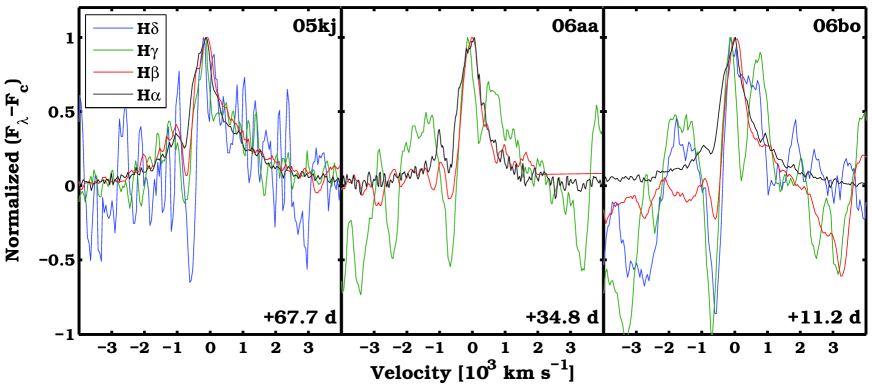
Figure 13: Over-imposed Balmer line profiles after continuum subtraction and peak normalization for SNe 2005kj, 2006aa, and 2006bo.

Each of our five objects discussed in the previous sections has prevalent H$\alpha$ and H$\beta$ features, which serve as the basis for their classification as bonafide SNe IIn. In three of them (SNe 2005kj, 2006aa, and 2006bo), the narrow Balmer lines show P-Cygni profiles that sit on top of broad and symmetric bases. In the three panels of Fig. 13, the Balmer lines of these three objects are compared after continuum-subtraction, extinction correction, and peak normalization. It turns out that for shorter wavelengths, the narrow absorption deepens. The broad component is likely produced by fast moving material that is associated with the underlying SN ejecta, but it might also be due to the electron scattering of the narrow line photons.

Concerning the narrow Balmer lines, their narrow P-Cygni profiles suggest that they arise from the recombination of a slow CSM that surrounds the SN rather than from an underlying H ii region. Only for SN 2006qq, the narrow Balmer absorption is not detected, and in these spectra, we also observe narrow emission from [N ii], which is typical of H ii regions. However, the absence of strong oxygen and sulfur emission lines suggests that the narrow emission in SN 2006qq is not only due to contamination, but also to ionization of the CSM.

Plotted in the left panel of Fig. 14 are the H$\alpha$ EW values for the full CSP SN IIn sample, along with those of several objects from the literature. For some objects, this parameter tends to increase over time, suggesting that the bulk of the radiation at early phases is related to continuum flux, whereas line emission dominates at later epochs. In particular, SNe 1998S and 2008fq standout, both showing a strong H$\alpha$ EW enhancement of 10 Å to 250 Å within the first 70 days of evolution. Other events, like SNe 2005kj and 2006aa, exhibit an almost constant H$\alpha$ EW. In Table 20, we report the EW values of our five objects.

We also examine the total H$\alpha$ luminosity, which is shown in the right panel of Fig. 14. $L$(H$\alpha$) values were computed by multiplying the de-reddened fluxes (presented in Figs. 8–12) by 4$\pi$D${}_{L}^{2}$, where D_L is the luminosity distance listed in Table 1. H$\alpha$ luminosities of our objects are comparable with the typical values found for SNe IIn in the literature.

Concerning other lines, it is known that SNe IIn can exhibit Fe ii and Ti ii P-Cygni profiles. Following the line identification presented by Kankare et al. (2012), these features are identified in moderately young spectra of SNe 2005kj, 2006aa, and 2006bo and shown in Fig. 15 (left panel). In SNe 2006qq and 2008fq, Fe ii features are present as well, although they appear heavily blended. As shown in the right panel of Fig. 15, the Ca ii NIR triplet is observed in neither SNe 2006aa nor 2006qq, is barely detected in SNe 2005kj and 2006bo, and is clearly observed in SN 2008fq, whose red portion of the spectrum is characterized by broad P-Cygni profiles.

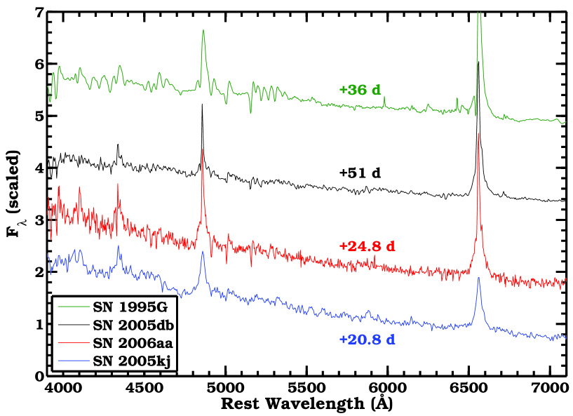
Figure 16: Spectral comparison between SNe 2005kj and 2006aa to SNe 2005db and 1995G.

All of our objects are found to be spectroscopically similar to other events that were previously reported in literature. In Fig. 16, we present a spectral comparison of SNe 2005kj and 2006aa to SNe 2005db (Kiewe et al. 2012) and 1995G (Pastorello et al. 2002). Each spectrum is corrected for reddening and presented in its rest frame. The spectra are mainly characterized by a combination of narrow and broad Balmer features. Fe ii lines are also present, modifying the bright blue continuum. The red continuum is almost featureless. Basically, the spectra of SNe 2005kj and 2006aa follow the definition of SN IIn provided by Schlegel (1990) and are similar to those of many other SNe IIn in the literature (e.g. SNe 1999eb and 1999el; see Fig. 8 of Pastorello et al. 2002).

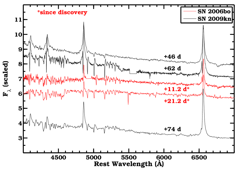
Figure 17: Spectral comparison between SN 2006bo and the 1994W-like SN 2009kn (Kankare et al. 2012).

SN 2006bo appears to fit well within the recently suggested Type IIn-P subclass (see Mauerhan et al. 2012a). The light curves presented in Sect. 4 show a luminosity drop after a plateau phase, which was also observed in SNe 1994W (Sollerman et al. 1998), 2009kn (Kankare et al. 2012), and 2011ht (Mauerhan et al. 2012a). The spectral comparison to SN 2009kn confirms that SN 2006bo is a similar object, as shown in Fig. 17. SN 2006bo spectra clearly resemble those of SN 2009kn $\approx$ 2 months after explosion (during the plateau phase). The common features are the narrow Balmer emission lines, along with the narrow Balmer absorption lines, and the Fe ii P-Cygni profiles.

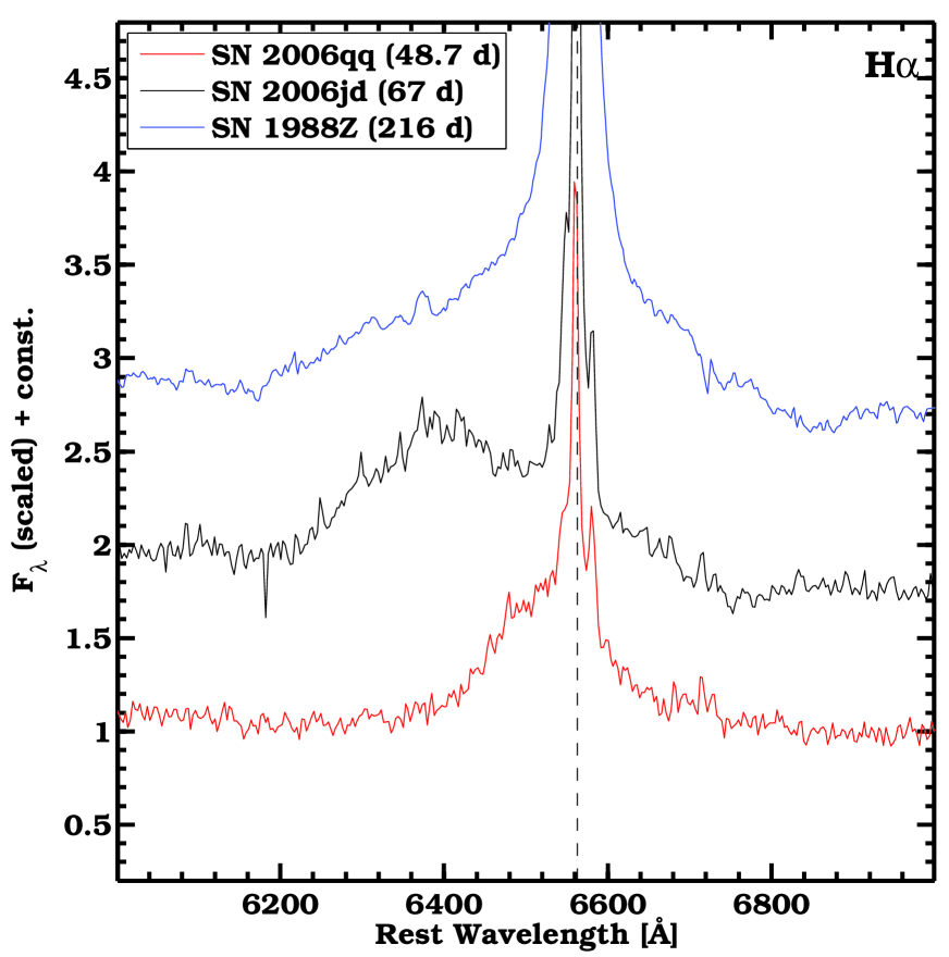
Figure 18: H$\alpha$ comparison between SNe 1988Z, 2006jd, and 2006qq. Each object exhibits preferential emission in the blue wing.

SN 2006qq is a peculiar object with its very broad emission features and its strong asymmetry in the H$\alpha$ profile. In Fig. 18, its H$\alpha$ profile is compared to those of SNe 1988Z (Turatto et al. 1993) and 2006jd (S12). Even though SN 2006qq clearly exhibits slower velocities in the broad component than those of SNe 1988Z and 2006jd, the profile is similarly characterized by a strong suppression of the red-wing. The fact that the broad H$\alpha$ component significantly strengthens weeks after explosion is similar to what was observed for SN 2006jd but on different timescales (for SN 2006jd, H$\alpha$ became remarkably brighter about 400 days after explosion).

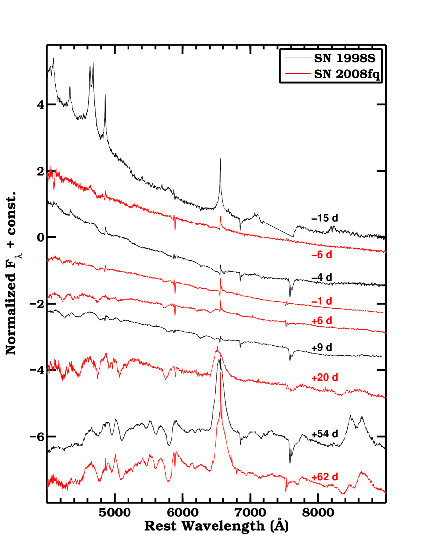
Figure 19: Spectral evolution of SNe 1998S and 2008fq. Temporal phase of each spectrum is given relative to the time of $V$-band maximum.

SN 2008fq can be defined as a SN 1998S-like event. SN 1998S is among the best-studied interacting SNe. A comparison of the spectral evolution of SNe 1998S and 2008fq is presented in Fig. 19. Here, the spectra were de-reddened, and the listed epochs are relative to the time of $V$-band maximum. The similarity between the two objects is remarkable at all epochs. We note that the light curves are also very similar, as demonstrated in Sect. 4. The first example of SNe similar to 1998S and 2008fq is actually SN 1983K (Niemela et al. 1985; Phillips et al. 1990), but a less extensive set of spectral and photometric observations exists for this object. SN 2005gl also shows a spectral evolution that resembles that of SN 1998S (Gal-Yam et al. 2007; Gal-Yam & Leonard 2009). Another object, which shares similar properties to SNe 1998S and 2008fq is SN 2007pk, which has recently been presented by Inserra et al. (2012). We note that SNe 2007pk and 2008fq show traces of C iii and N iii emission that were strong at early epochs for both SNe 1983K and 1998S. Finally, the late-time spectra ($\geq$232 days) of SN 2007od (Andrews et al. 2010) are similar to those of SN 1998S. Interestingly, the absolute magnitudes of the above-mentioned events are also similar, ranging between $V_{\max}\sim$ $-$18.5 mag (SN 2007pk) and $V_{\max}\sim$ $-$19.3 mag (SN 2008fq). These values are affected by large uncertainties on the extinction.

6 Discussion

In the following, we discuss the data for each of the five new CSP SNe IIn to determine the likely scenario underlying each object. Consistent with the interpretation of other SNe IIn, we assume that the ejecta of the exploding progenitor stars are experiencing strong interaction with surrounding CSM. In the following, constraints are placed on the mass-loss rate, the density, and the extent of the CSM for each SN. Estimates derived in the following section are summarized in Table 21, which also includes the corresponding values derived from observations of SNe 2005ip and 2006jd. We stress that the mass-loss rate estimates are based on the uncertain assumption that the progenitor wind was steady. Therefore, the more robust density wind parameter $w$ = $\dot{M}v_{w}^{-1}$ is also reported in Table 21.

6.1 SN 2005kj

The explosion date of SN 2005kj is not well constrained by pre-explosion images (see Table 2). However, its light curves were probably observed only a few days after maximum, which can be inferred from their flattening at early epochs. The high (approximately 10,000 K) early-time temperatures determined by BB fits and presented in Fig. 7 (middle panel) also suggest that the observations began soon after explosion. Based on the temperature comparison between SN 2005kj to SN 2008fq, we assume here that the explosion of SN 2005kj occurred 8 days prior to its discovery.

The high-energy radiation produced via shock interaction ionizes the slow moving CSM and gives rise to observed narrow (FWHM_n $\approx$ 1000 km s^-1) Balmer emission lines through recombination. The narrow Balmer absorption feature, appearing a couple of months after discovery (well visible in H$\beta$), is also likely produced within the slow-moving CSM ($v_{min}$ $\approx$ 600 km s^-1).

SN 2005kj presents iron and hydrogen P-Cygni profiles that are rounded and symmetric. The same properties were observed in the spectra of SN 1994W (Sollerman et al. 1998) and SN 1995G (Pastorello et al. 2002). Because of that, line optical depths of $\tau$ $>$1 were inferred for both objects, which allows the use of the expression n_H $>$ 3 $\times$ 10⁸ v₃ r${}_{15}^{-1}$ cm^-3 (Mihalas 1978) to estimate the electron density of the CSM. Here, r₁₅ is the CSM shell radius, which is close to the photospheric radius (expressed in units of 10¹⁵ cm, from BB fits to the SED); v₃ is the CSM shell velocity measured from the narrow P-Cygni absorption minimum and given in units of 10³ km s^-1. We use the same expression for SN 2005kj (v₃ $\approx$ 0.6 and r₁₅ $\approx$ 1), obtaining a lower limit for the CSM electron density: n_H $>$ 1.8$\times$10⁸ cm^-3.

Clear signs of CSI are observed from the epoch of the first spectrum to the epoch of the last one (approximately 170 days since explosion), which means the ejecta did not overtake the outer radius of the CSM in 170 days. If the fastest ejecta were moving at $v^{\rm max}_{\rm ejecta}$ $\approx$ 3000 km s^-1 (BVZI of the broad component of H$\alpha$), this would then suggest that the outer radius of the CSM is $R_{\rm CSM}^{\rm out}$ $\gtrsim$ 4.4$\times$10¹⁵ cm. Given that the interaction is already present at $\approx$ 15 days after explosion, the inner radius of the CSM is $R_{\rm CSM}^{\rm in}$ $<$ 0.4$\times$10¹⁵ cm.

Following Salamanca et al. (1998), a rough estimate of the mass-loss rate ($\dot{M}$) can be computed via: $L$(H$\alpha_{\rm broad}$) $\approx$ 0.25$\epsilon_{\rm H\alpha}\dot{M}v_{s}^{3}v_{w}^{-1}$, which is based on the assumption that the wind forming the CSM is steady. Here we adopted the shock velocity $v_{s}$ $\approx$ 3000 km s^-1, which is derived from the FWHM of the broad component, and the wind velocity of $v_{w}$ $\approx$ 600 km s^-1, which is obtained from the minimum of the narrow P-Cygni absorption. The efficiency factor is assumed to be $\epsilon_{\rm H\alpha}$ $=$ 0.1, which is found in the literature (see e.g Kiewe et al. 2012). The broad H$\alpha$ luminosity is measured to be $L$(H$\alpha_{\rm broad}$) $\approx$ 1.0$-$3.4$\times$10⁴⁰ erg s⁻¹. From these values, we obtain $\dot{M}$ $\approx$ 1.4$-$4.8$\times$10^-3 $M_{\odot}$ yr^-1.

6.2 SN 2006aa

SN 2006aa was discovered before maximum luminosity and its explosion date is well constrained (uncertainty of $\pm$8 days) thanks to pre-explosion images. We therefore assume the core collapse occurred 8 days before discovery (see Table 2).

The spectra and the bolometric light curve suggest that the main source of energy is CSI, rather than the radioactive decay of ⁵⁶Ni and ⁵⁶Co. If we naively assume that the peak luminosity is powered solely due to radioactive decay, the combinination of the epoch of the peak and the peak bolometric luminosity with Arnett’s rule (Arnett 1982; Arnett et al. 1985; Branch 1992) gives a ⁵⁶Ni mass $=$ 0.3 $M_{\odot}$. This value is large compared to the typical ⁵⁶Ni masses measured for SNe II (see Figure 9 in Smartt et al. 2009).

BB fits of the SEDs reveal that the peak temperature was reached close to maximum light – i.e, around 60 days after explosion. This late-time peak and the initial rise of the temperature can be explained by a strengthened interaction due to the presence of a dense shell of CSM. Given that the maximum ejecta velocity is $v^{\rm max}_{\rm ejecta}$ $\approx$ 2500 km s^-1 (BVZI of H$\alpha$) and $t_{\rm max}$ $\approx$ 60 days, the densest part of the CSM is likely located at $R_{\rm CSM}^{\rm sh}$ $\approx$ 1.3$\times$10¹⁵ cm. Since the wind velocity, which is derived from the narrow P-Cygni absorption minimum, is $\approx$ 600 km s^-1, the mass-loss episode that produces this dense shell likely occurred $\approx$ 8 months prior to core collapse.

As the spectra of SN 2006aa are quite similar to those of SN 2005kj, similar techniques can be adopted to estimate the electron density of the wind, the physical extension in radius from the progenitor of the CSM, and the progenitor’s mass-loss rate. We obtain n_H $>$ 7.6$\times$10⁸ cm^-3 by assuming v₃ $\approx$ 0.6 and r₁₅ $\approx$ 0.8. The inner CSM radius is $R_{\rm CSM}^{\rm in}$ $<$ 0.5$\times$10¹⁵ cm, and the outer one is $R_{\rm CSM}^{\rm out}$ $\gtrsim$ 1.8$\times$10¹⁵ cm, assuming the above mentioned value of $v^{\rm max}_{\rm ejecta}$ and the interaction begins 24 and ends 85 days after explosion.

The mass-loss rate is $\dot{M}$ $\approx$ 5.4$-$16.2$\times$10^-3 $M_{\odot}$ yr^-1, where a wind velocity $v_{w}$ $\approx$ 600 km s^-1 and a shock velocity $\approx$ 2000 km s^-1 (FWHM_b) were used. The efficiency factor is again assumed to be $\epsilon_{\rm H\alpha}$ $=$ 0.1. The broad H$\alpha$ luminosity is found to be $L$(H$\alpha_{\rm broad}$) $\approx$ 1.1$-$3.4$\times$10⁴⁰ erg s^-1.

6.3 SN 2006bo

The explosion date of SN 2006bo is not well constrained by pre-explosion images. Since we observed a plateau in the light curve having a duration of about 70 days and then observed a sudden drop in luminosity, we classify SN 2006bo as a SN 1994W-like event. These transients are characterized by a 100 days plateau; therefore, it is possible that SN 2006bo was discovered even a month after explosion. Because we did not observe the SN between 70 and 145 days after discovery, it makes impossible to know whether the drop in luminosity occurred immediately after 70 days or later, and therefore, a proper comparison of the plateau’s length is difficult. On the other hand, the spectral comparison to SN 2009kn shown in Fig. 17 suggests that the SN could have been discovered at least 40 days after explosion. The large uncertainty on the explosion date determines the uncertainty on the amount of ⁵⁶Ni that is likely to power the light curve tail, which was the case in SN 2009kn (Kankare et al. 2012). Assuming that the explosion occurred on the day of discovery, the bolometric light curve tail then yields a ⁵⁶ Ni mass of $M_{\rm{}^{56}Ni}$ $=$ 0.007$M_{\odot}$. If the explosion occurred 40 days before, then a $M_{\rm{}^{56}Ni}$ $=$ 0.011$M_{\odot}$ is obtained. In any case, that value would be lower than the upper limit estimated for SN 2009kn of 0.023 $M_{\odot}$ (Kankare et al. 2012) and comparable to the value 0.01 $M_{\odot}$, inferred for SN 2011ht (Mauerhan et al. 2012a). Unfortunately, it is not possible to determine if the slope of the SN tail is consistent with the ⁵⁶Co decay, since only a single photometric epoch was obtained at late epochs.

The Balmer lines appearing in the two spectra of SN 2006bo seem to be well reproduced by the addition of a single Lorentzian function, with typical FWHM $\approx$ 1000 km s^-1 and an absorption component that peaks at $-$600 km s^-1. We believe that both components are generated in the CSM with wind velocity $v_{w}$ $\approx$ 600 km s^-1. The reason that the narrow emission component has slightly higher velocities than the narrow absorption might be due to the electron-scattering broadening of the narrow emission in the wind. The likely absence of a broad component might mean that ionized ejecta are not visible because of a CDS (cold-dense-shell). Given that we do not observe the broad component, we assume the shock velocity to have a lower limit equal to the FWHM of the narrow component, i.e. $v_{s}$ $\gtrsim$ 1000 km s^-1.

The duration of the plateau is 70$-$110 days, which means the outer radius of the CSM surrounding SN 2006bo is $R_{\rm CSM}^{\rm out}$ $\approx$ 1.5$-$2.4$\times$10¹⁵ cm. We assume here that the emission after the plateau phase is mainly due to radioactive decay rather than to CSI and a maximum ejecta velocity of $v^{\rm max}_{\rm ejecta}$ $\approx$ 2500 km s^-1 (BVZI of H$\alpha$). The limit on the inner CSM radius is computed from the epoch of the first spectrum (11$-$41 days depending on the explosion date). We obtain $R_{\rm CSM}^{\rm in}$ $\approx$ 0.2$-$0.9$\times$10¹⁵ cm.

The mass-loss rate estimate gives $\dot{M}$ $\lesssim$ 2.28$-$3.42$\times$10^-2 $M_{\odot}$ yr^-1. We assume here that the total H$\alpha$ luminosity is the upper limit value for the broad H$\alpha$ luminosity, $L$(H$\alpha_{\rm broad}$) $\lesssim$ 0.6$-$0.9$\times$10⁴⁰ erg s^-1, using the mentioned values of $\epsilon_{\rm H\alpha}$, $v_{s}$ and $v_{w}$. For a photospheric radius of 7.9$\times$10¹⁴ cm (see Fig. 7, bottom panel), the electron density is n_H $>$ 3.8$\times$10⁸ cm^-3.

6.4 SN 2006qq

SN 2006qq was discovered relatively soon after explosion. Given the constraint from the pre-explosion images, we assume the explosion occurred 16 days before discovery (see Table 2). This appears consistent with the temperature comparison to SN 2008fq (see Fig. 7, middle panel), whose explosion date is better constrained, although the temperature evolution is hard to standardize.

Given the bright emission lines, it is likely that CSI powers the emission of SN 2006qq, although the bolometric light curve seems to follow the ⁵⁶Co radioactive decay at late times. If radioactive decay was the main powering source at late times, a ⁵⁶Ni mass of $M_{\rm{}^{56}Ni}$ $=$ 0.4 $M_{\odot}$ is derived.

As discussed in Sect. 5, the spectra reveal strong, broad H$\alpha$ and H$\beta$ emission from the ionized ejecta, whose luminosity reaches its maximum at 76 days after explosion. The broad emission from the ejecta is strongly asymmetric, where H$\alpha$ BVZI $\approx$ 10⁴ km s^-1 and RVZI $\approx$ 3$\times$10³ km s^-1. The asymmetry can be explained in terms of dust obscuration of the radiation coming from the back of the ejecta. Indeed, Fox et al. (2011) detected 0.5$-$1.7$\times$10^-2 $M_{\odot}$ of (graphite) dust emitting in the MIR for this SN. The strong asymmetric H$\alpha$ profile can also be produced through the occultation of the radiation that comes from the receding ejecta by an opaque photosphere. The ratio between the photospheric radius and the maximum ejecta radius ($R_{\rm p}/R_{\rm max}$) can be determined from H$\alpha$ BVZI and RVZI for each spectral epoch (see S12). In this case, we obtain $R_{\rm p}/R_{\rm max}$ $\approx$ 0.87 at 28 days and $R_{\rm p}/R_{\rm max}$ $\approx$ 0.95 at 76 days after explosion.

The epoch of the maximum broad emission and the maximum ejecta velocity ($v^{\rm max}_{\rm ejecta}$, from the H$\alpha$ BVZI) set the distance ($R_{\rm CSM}^{\rm sh}$) to the densest part of the CSM, which is $R_{\rm CSM}^{\rm sh}$ $\approx$ 6.6$\times$10¹⁵ cm. This dense shell was ejected during the end of the life of the progenitor star. If the wind velocity is $v_{w}$ $\lesssim$ 200 km s^-1, as measured from the FWHM of the narrow emission lines, then the mass-loss episodes that produced the dense shell occurred at least 10 years before core collapse. With the assumed $v_{w}$ and $v_{s}$ $\approx$ 6000 km s^-1 (that corresponds to the broad H$\alpha$ FWHM if we neglect the occultation effect), the broad H$\alpha$ luminosity gives a mass-loss rate of $\dot{M}$ $\lesssim$ 0.3$-$0.7$\times$ 10^-3 $M_{\odot}$ yr^-1. We derive an electron density lower limit of n_H $>$ 1.1$\times$10⁹ cm^-3 from a photospheric radius of 1.6$\times$10¹⁵ cm. The inner and the outer CSM radii that we can probe correspond to the phase of the first and the last spectral epoch (29 and 91 days since explosion, respectively) multiplied by $v^{\rm max}_{\rm ejecta}$. We obtain $R_{\rm CSM}^{\rm in}$ $\lesssim$ 2.5$\times$10¹⁵ cm and $R_{\rm CSM}^{\rm out}$ $\gtrsim$ 7.9$\times$10¹⁵ cm.

6.5 SN 2008fq

The explosion date of SN 2008fq is well constrained by pre-explosion images ($\pm$4.5 days uncertainty). The light curve comparison with SN 1998S (see bottom panel of Fig. 5) suggests that the explosion occurred soon after the last non-detection, approximately 8 days before discovery. The presence of broad H$\alpha$ P-Cygni features in the early time spectra allows us to estimate the ejecta velocity; we obtain $v_{min}=$7000$-$8000 km s^-1. Given that the first spectrum was observed 1.7 days after discovery and that the photospheric radius at that epoch was approximately 10¹⁵ cm, we confirm that the core collapse occurred soon after the last non-detection by assuming free expansion.

The lack of a very early time spectrum prevents us from determining if SN 2008fq displayed strong CSI soon after core collapse, as was observed in SN 1998S (Leonard et al. 2000; Fassia et al. 2001, and see strong emission lines in the spectrum of SN 1998S at 15 days from its in Fig. 19). The presence of a wind moving at $v_{w}$ $\approx$ 500 km s^-1 (from the narrow absorption minimum) is observed in SN 2008fq, as was also detected for SN 1998S at similar phases (Leonard et al. 2000; Fassia et al. 2001). We note, however, that the wind velocity of SN 1998S was lower ($\approx$ 150 km s^-1). From the extreme blue edge of the broad H$\alpha$ absorption, we determine a maximum ejecta velocity $v^{\rm max}_{\rm ejecta}$ $\approx$ 9000 km s^-1. If we assume that SN 2008fq had an inner CSM (ICSM) like that of SN 1998S (Leonard et al. 2000; Fassia et al. 2001), with the first spectrum observed approximately 10 days after explosion and the above mentioned $v^{\rm max}_{\rm ejecta}$, the ICSM could not be more extended than $R_{\rm CSM}^{\rm in}$ $\approx$ 7.8$\times$10¹⁴ cm.

As shown in Sect. 5, a broad, prevalent Balmer emission component emerges about 20 days after maximum (45 days after explosion). Following the interpretation of Leonard et al. (2000); Fassia et al. (2001) for SN 1998S, this is likely due to the interaction with an outer, denser CSM (OCSM). Given the assumed $v^{\rm max}_{\rm ejecta}$, the inner part of the OCSM is placed at $R_{\rm CSM}^{\rm sh}$ $\approx$ 3.5$\times$10¹⁵ cm. A similar inner radius was found for the OCSM of SN 1998S (Fassia et al. 2001). The outer radius of the OCSM corresponds to the last spectral epoch (78 days after explosion); we obtain $R_{\rm CSM}^{\rm out}$ $\gtrsim$ 6.1$\times$10¹⁵ cm. Given these radii and the assumed wind velocity, the OCSM was ejected during an episodic mass loss that started at least 3.9 years before core collapse and ended 2.2 years prior to core collapse. Assuming the same wind velocity, the ICSM was formed during a mass-loss that started less than 6 months before core collapse.

The most likely scenario is that the observed spectra up to 6 days after maximum are mainly powered by the ejecta interaction with a low-density, mid-CSM (MCSM). As suggested by Fassia et al. (2001) for SN 1998S, this would explain the low contrast of the P-Cygni profiles (formed in the ejecta) on the blue continuum of the spectra (produced in a cold dense shell at the ejecta/MCSM interface). Only 20 days after maximum, the ejecta reach the OCSM, giving rise to a stronger interaction.

The mass-loss history of SN 2008fq is likely characterized by episodic outbursts that gave rise to a complex CSM. Therefore, an estimate of the mass-loss rate is difficult to obtain as the steady wind hypothesis is likely wrong. If we assume the shock velocity to be similar to the ejecta velocity $v_{min}$ (consistently with the FWHM of the broad H$\alpha$ component in the last spectra), the above-mentioned $v_{w}$ and $L$(H$\alpha$)_broad $\approx$ 1.5$\times$10⁴¹ erg s^-1, however, we obtain $\dot{M}$ $\approx$ 1.1$\times$ 10^-3 $M_{\odot}$ yr^-1. We also obtain n_H $>$ 9.0$\times$10⁸ cm^-3 (for a typical photospheric radius R_ph $\approx$ 2.5$\times$10¹⁵ cm).

6.6 SN IIn subtypes and progenitor scenarios

The seven CSP SNe IIn confirm the diversity of observational properties from this subclass of CC explosions, while the case of SN 2006aa displays previously unobserved properties. Under close examination, these objects show how SNe IIn can be separated out into different categories.

SN 2006bo belongs to the rare SN 1994W-like class (Mauerhan et al. 2012a). Besides SN 1994W (Sollerman et al. 1998), only two additional objects are known to belong to this group, namely SNe 2009kn (Kankare et al. 2012) and 2011ht (Mauerhan et al. 2012a). These objects all have Type IIn spectral features but they also present a characteristic light curve plateau phase, like that observed in SNe IIP.

With a few other objects (e.g. SNe 2007pk and 1983K) SN 2008fq forms the SN 1998S-like category, which presents optical light curves that peak within 10$-$20 days at $-$18.5 $\lesssim$ $V_{\rm max}$ $\approx$ $\lesssim$ $-$19.3 mag, and which displays characteristic spectral evolution with broad emission components that arise after maximum light. SN 2006qq, SNe 2005ip, and 2006jd (S12) resemble the Type IIn SNe 1988Z and 1995N (Turatto et al. 1993; Fransson et al. 2002). Evidently, two common properties among these objects are an asymmetric H$\alpha$ profile and long-lasting dust emission that peaks at MIR wavelengths.

SNe 2005kj is similar to the more common SNe IIn, like those presented in Kiewe et al. (2012) (e.g. SN 2005cp). SN 2006aa shows an interesting and unprecedented initial plateau in the $u$ band and an uncommon late time increase of the photospheric temperature. Like SN 2005kj, its spectral features are however similar to those of typical SNe IIn (Kiewe et al. 2012).

We note that the initial class of Type IIn SNe (Schlegel 1990) is likely to include a variety of phenomena with the common characteristics of CSI giving rise to narrow Balmer lines. Some subtypes have already been identified and singled out in the past, and we note that some of these rare interacting, core-collapse SN types are not represented in the CSP sample, like superluminous SNe-II (Gal-Yam 2012) and SNe Ibn (Pastorello et al. 2008). A couple of SN 2002ic-like objects (Hamuy et al. 2003) were observed by the CSP and presented in Prieto et al. (2007) and Taddia et al. (2012). These events show spectra resembling those of SNe Ia, although diluted by a blue continuum with the addition of Balmer emission lines. These properties can be interpreted as the result of the interaction between a thermonuclear SN and its dense CSM. Following this interpretation, we believe these transients do not belong to the family of core-collapse SNe IIn, and therefore we do not include them in our sample. However, we note that alternative explanations support the idea that SN 2002ic-like objects might actually be core-collapse events (Benetti et al. 2006).

Smith et al. (2011) found that the SNe IIn subclass constitutes about 9 percent of all CC SNe. Although the CSP was not an unbiased survey, the number of SNe IIn (7) and the total number of CC SNe (116) is consistent with the fraction found by Smith et al. (2011). As noted by Kiewe et al. (2012), who added 4 more SNe IIn, the current number of well studied SNe IIn is still very low, and often publications are driven by more peculiar objects. The CSP sample presented here therefore contributes significantly to the current Type IIn sample.

Although our sample is still too small to allow further subclassifications, all the objects we have found do match up with similar objects in the literature, even if there is large diversity in the properties of SNe IIn. It thus seems that the population of narrow-line CC SNe separate out into discrete subcategories. This is based on only a handful of objects, and further observations are clearly needed to map out the diversity of SNe IIn.

What determines the appearance of these objects is foremost the mass-loss history, since this shapes the CSM with which the SN interacts. For line-driven stellar winds, the main factors that affect the mass-loss are the progenitor mass and the metallicity. If that was the main mass-loss mechanism, then we could expect a continuum of observational properties, which reflect the continuous variation of progenitor mass and metallicity. However, SN 1994W-like, SN 1998S-like, and long-lasting SNe IIn look distinctively different, and we have not yet found any transitional or intermediate objects that connect these different subtypes. This could imply that the final fate of these stars can only follow certain specific paths.

One overall aim of continued studies of SNe IIn is to identify the progenitor stars that end their lives following these paths. This is often done by comparing the derived mass-loss properties with those of massive stars. In this regard, we note some caveats.

The mass-loss rate estimates that we have presented assume steady winds. This makes them easy to calculate from the observables, and easy to compare to many similar estimates in the literature. It should be emphasized, however, that this is likely a much too simplistic assumption (e.g Dwarkadas 2011). Much of the observations of SNe IIn seem to favor mass-loss histories of more complicated kinds, including clumped winds and ejected shells. The wind density parameters presented in Table 21 are more closely tied to the observations, which are independent from wind velocities.

We also remind the reader that the mass-loss period probed by observations of SNe IIn is only a very tiny fraction of the lifetime of the progenitor stars. What we know observationally about the mass-loss properties of RSG or LBV stars is derived from stars that are not that close ($\lesssim$ 1000 years) to their final explosion.

If the mass-loss history in SNe IIn was dominated by other mechanisms, like pulsations (Yoon & Cantiello 2010), which drive episodic outbursts occurring only under specific conditions, we could more easily explain the existence of such different subtypes. Our sample does imply that dense shells have likely been ejected soon before explosion by episodic outbursts, at least for some SNe (2006aa, 2006jd, 2006qq, and 2008fq).

The values derived for the mass-loss rates in this work (10^-4–10^-2 $M_{\odot}$ yr^-1) are similar to those found by Kiewe et al. (2012) for other SNe IIn. Such high numbers may imply that LBVs are the most likely progenitor channel, but it is unclear if RSG may not also produce some of the events when the steady wind assumption is not enforced. The wind density parameter of three SNe in our sample is higher than 10¹⁶ g cm^-1; the other objects exhibit $w$ $\sim$ 10¹⁵ g cm^-1. These values are consistent with those found for other events in the literature (e.g. Chugai & Danziger 1994; Smith et al. 2009a).

There are certainly objects like SN 2005gl (Gal-Yam & Leonard 2009) and SN 2009ip (Mauerhan et al. 2012b; Pastorello et al. 2012) with identified LBV progenitors; in these cases, the progenitor was directly detected before core collapse. However, we caution that other channels (like RSGs) cannot be excluded on the basis of rough mass-loss rate estimates. Interestingly, Anderson et al. (2012) show that SNe IIn are located in environments similar to those of SNe IIP (whose progenitors are RSGs), indicating that the majority of events may not arise from very massive stars like LBVs.

The estimates of wind velocities from the narrow P-Cygni absorption features (for our sample, we find typical values of 500–600 km s^-1) are also consistent with LBV wind velocities. However, slower winds might have been accelerated at the shock breakout by the radiation pressure. In that case, we would detect velocities of hundreds of km s^-1, even though the wind had an original velocity of tenths of km s^-1 (such as those measured for RSGs).

7 Conclusions

In this paper, we have presented the data for five of the seven CSP SNe IIn, including extensive optical and NIR photometry and visual-wavelength spectroscopy. We confirm the diversity of this class of SNe, although a comparison to objects in the literature provides counterparts for each object. This implies that several subcategories are present within the SNe IIn class, including SN 1994W-like (SN 2006bo), SN 1998S-like (SN 2008fq) and SN 1988Z-like (SN 2006qq) events. These subcategories appear significantly different from each other, suggesting that SNe IIn might be the result of different conditions in the progenitor mass/metallicity phases space. With a late-time maximum and an initial $u$-band plateau, the peculiar SN 2006aa was also studied. Estimates for CSM parameters have been derived and compared to objects in the literature. Mass-loss rates and wind velocities derived from this sample are compatible with LBV progenitors, although caveats of such a connection are discussed.

Table 1: Full CSP sample of SNe IIn.

SN	RA	DEC	Galaxy	Galaxy	Redshift	Distance	$E(B-V)_{\rm MW}$	$E(B-V)_{\rm host}$	EW$(\rm{Na\textsc{i}}\leavevmode\nobreak\ D)_{\rm h}$
				Type		(Mpc)	(mag)	(mag)	(Å)
2005ip	09:32:06.42	$+$08:26:44.4	NGC 2906	Scd	0.0071	34.9$\pm$0.6	0.042	…	…
2005kj	08:40:09.18	$-$05:36:02.2	A084009-0536	$\cdots$	0.0170	77.3$\pm$1.5	0.025	…	…
2006aa	11:53:19.89	$+$20:45:18.2	NGC 3947	SBb	0.0207	97.5$\pm$1.8	0.036	…	…
2006bo	20:30:41.90	$+$09:11:40.8	UGC 11578	Sdm	0.0153	70.0$\pm$1.3	0.091	…	…
2006jd	08:02:07.43	$+$00:48:31.5	UGC 4179	SBb	0.0186	83.8$\pm$1.5	0.048	…	…
2006qq	05:19:50.43	$-$20:58:06.4	E553-G36	Sb	0.0290	125.0$\pm$2.3	0.034	0.12$\pm$0.03	0.76$\pm$0.21
2008fq	20:25:06.20	$-$24:48:28.00	NGC 6907	SB(s)bc	0.0106	49.6$\pm$0.9	0.056	0.46$\pm$0.03	2.90$\pm$0.20

Table 2: Discovery Telegrams.

SN	Discovery	Classification	Last non detection	Discovery	Explosion date
	telegram	telegram	JD$-$2453000	JD$-$2453000	JD$-$2453000
2005ip	CBET 275	CBET 276	391.50	679.66	535.58$\pm$144.08
2005kj	CBET 296	CBET 296	$\cdots$	692.00	$\cdots$
2006aa	CBET 395	ATel 732	758.99	774.98	766.99 $\pm$8.00
2006bo	CBET 468	CBET 481	702.5 0	830.65	766.58 $\pm$64.07
2006jd	CBET 673	CBET 679	846.7	1021.04	933.87$\pm$ 87.17
2006qq	CBET 766	CBET 766	1035.90	1069.87	1052.89$\pm$16.98
2008fq	CBET 1507	CBET 1510	1715.80	1724.79	1720.29$\pm$4.49

3

Table 3: Optical and near-infrared photometry of the local sequences in the standard system

			$u^{\prime}$	$g^{\prime}$	$r^{\prime}$	$i^{\prime}$	$B$	$V$	$Y$	$J$	$H$	$K_{s}$
STAR	$\alpha(2000)$	$\delta(2000)$	(mag)	(mag)	(mag)	(mag)	(mag)	(mag)	(mag)	(mag)	(mag)	(mag)
SN 2005kj
01	08:40:14.48	$-$05:35:21.98	$\cdots$	$\cdots$	$\cdots$	$\cdots$	14.142(016)	$\cdots$	$\cdots$	$\cdots$	$\cdots$	$\cdots$
02	08:40:06.53	$-$05:37:07.63	$\cdots$	$\cdots$	$\cdots$	$\cdots$	$\cdots$	$\cdots$	$\cdots$	$\cdots$	$\cdots$	$\cdots$
03	08:40:05.50	$-$05:37:05.35	15.772(015)	$\cdots$	$\cdots$	$\cdots$	14.555(009)	13.753(014)	12.616(005)	12.348(016)	11.932(005)	$\cdots$
04	08:39:59.04	$-$05:36:21.37	$\cdots$	$\cdots$	$\cdots$	$\cdots$	$\cdots$	$\cdots$	$\cdots$	$\cdots$	$\cdots$	$\cdots$
05	08:40:16.65	$-$05:37:38.33	15.540(015)	14.434(015)	14.189(015)	14.133(015)	14.710(008)	14.270(008)	13.639(005)	13.457(005)	13.239(005)	$\cdots$
06	08:39:59.30	$-$05:33:06.59	16.148(010)	14.931(007)	14.534(007)	14.394(008)	15.282(008)	14.685(007)	$\cdots$	$\cdots$	$\cdots$	$\cdots$
07	08:40:09.91	$-$05:32:33.87	16.671(008)	15.326(007)	14.847(007)	14.673(009)	15.715(008)	15.039(007)	14.047(007)	13.775(007)	13.419(010)	$\cdots$
08	08:40:18.33	$-$05:37:23.79	16.433(008)	15.277(007)	14.961(007)	14.875(008)	15.580(008)	15.076(007)	14.328(006)	14.117(005)	13.851(006)	$\cdots$
09	08:39:58.25	$-$05:37:37.49	17.131(019)	15.576(007)	15.034(007)	14.814(008)	16.002(008)	15.249(007)	$\cdots$	$\cdots$	$\cdots$	$\cdots$
10	08:40:04.83	$-$05:33:04.74	17.201(017)	16.043(007)	15.682(007)	15.567(009)	16.378(008)	15.820(007)	15.017(007)	14.800(007)	14.507(011)	$\cdots$
11	08:40:13.98	$-$05:36:32.59	17.353(013)	16.164(007)	15.739(007)	15.597(010)	16.517(008)	15.899(007)	15.003(005)	14.761(006)	14.424(005)	14.384(015)
12	08:40:14.29	$-$05:39:07.22	17.907(027)	16.395(007)	15.847(007)	15.647(007)	16.834(008)	16.068(007)	14.967(007)	14.670(010)	14.269(006)	$\cdots$
13	08:40:06.11	$-$05:38:50.08	17.897(039)	16.421(007)	15.955(007)	15.813(008)	16.828(008)	16.135(007)	15.217(005)	14.970(005)	14.656(007)	$\cdots$
14	08:40:01.31	$-$05:37:38.36	17.851(017)	16.468(007)	15.994(007)	15.827(007)	16.859(008)	16.185(007)	$\cdots$	$\cdots$	$\cdots$	$\cdots$
15	08:40:22.60	$-$05:35:12.62	17.864(019)	16.587(007)	16.148(007)	15.985(010)	16.961(009)	16.312(007)	15.373(005)	15.119(005)	14.770(005)	$\cdots$
16	08:40:14.45	$-$05:32:31.58	18.027(022)	16.631(008)	16.160(007)	15.992(008)	17.010(008)	16.341(009)	$\cdots$	$\cdots$	$\cdots$	$\cdots$
17	08:40:10.94	$-$05:34:14.92	18.038(027)	16.664(007)	16.213(007)	16.070(008)	17.052(008)	16.388(007)	15.480(005)	15.227(005)	14.897(007)	$\cdots$
18	08:40:07.61	$-$05:38:09.01	19.131(064)	17.137(007)	16.342(007)	16.061(008)	17.660(017)	16.697(007)	15.277(006)	14.934(008)	14.430(006)	$\cdots$
19	08:40:16.87	$-$05:35:30.14	18.484(029)	17.218(008)	16.817(007)	16.681(007)	17.565(011)	16.965(007)	$\cdots$	$\cdots$	$\cdots$	$\cdots$
20	08:40:15.64	$-$05:34:50.35	18.768(037)	17.353(013)	16.861(009)	16.698(007)	17.772(008)	17.061(007)	$\cdots$	$\cdots$	$\cdots$	$\cdots$
21	08:40:08.45	$-$05:32:57.14	19.018(048)	17.749(007)	17.300(007)	17.152(011)	18.125(014)	17.480(007)	$\cdots$	$\cdots$	$\cdots$	$\cdots$
22	08:40:17.46	$-$05:34:09.57	18.867(226)	17.845(009)	17.357(009)	17.187(010)	18.235(013)	17.554(013)	$\cdots$	$\cdots$	$\cdots$	$\cdots$
23	08:40:05.58	$-$05:33:42.42	20.211(156)	18.227(010)	17.537(010)	17.288(010)	18.756(030)	17.831(013)	$\cdots$	$\cdots$	$\cdots$	$\cdots$
24	08:40:12.45	$-$05:35:51.28	$\cdots$	$\cdots$	$\cdots$	$\cdots$	$\cdots$	$\cdots$	15.009(005)	14.756(007)	14.418(006)	14.314(017)
25	08:40:07.12	$-$05:36:18.91	$\cdots$	$\cdots$	$\cdots$	$\cdots$	$\cdots$	$\cdots$	16.227(006)	15.792(008)	15.236(007)	15.070(048)
26	08:40:07.76	$-$05:36:34.89	$\cdots$	$\cdots$	$\cdots$	$\cdots$	$\cdots$	$\cdots$	16.071(007)	15.658(007)	15.052(006)	14.900(080)
27	08:40:10.34	$-$05:35:14.26	$\cdots$	$\cdots$	$\cdots$	$\cdots$	$\cdots$	$\cdots$	16.723(008)	16.379(010)	15.862(010)	15.679(066)
28	08:40:13.00	$-$05:35:14.74	$\cdots$	$\cdots$	$\cdots$	$\cdots$	$\cdots$	$\cdots$	16.716(007)	16.300(009)	15.685(010)	15.419(039)
29	08:40:07.65	$-$05:35:03.76	$\cdots$	$\cdots$	$\cdots$	$\cdots$	$\cdots$	$\cdots$	17.548(017)	17.125(014)	16.548(024)	16.224(054)
30	08:40:04.51	$-$05:36:51.69	$\cdots$	$\cdots$	$\cdots$	$\cdots$	$\cdots$	$\cdots$	17.240(016)	16.962(020)	16.514(035)	16.414(056)
31	08:40:17.07	$-$05:36:12.80	$\cdots$	$\cdots$	$\cdots$	$\cdots$	$\cdots$	$\cdots$	15.322(005)	14.834(005)	14.286(005)	$\cdots$
32	08:40:16.31	$-$05:36:01.90	$\cdots$	$\cdots$	$\cdots$	$\cdots$	$\cdots$	$\cdots$	15.957(005)	15.661(006)	15.264(010)	$\cdots$
33	08:40:30.21	$-$05:34:43.65	$\cdots$	$\cdots$	$\cdots$	$\cdots$	$\cdots$	$\cdots$	14.308(005)	13.875(006)	13.243(005)	$\cdots$
34	08:40:29.67	$-$05:37:15.36	$\cdots$	$\cdots$	$\cdots$	$\cdots$	$\cdots$	$\cdots$	12.496(006)	12.279(006)	12.003(005)	$\cdots$
35	08:40:31.93	$-$05:36:53.58	$\cdots$	$\cdots$	$\cdots$	$\cdots$	$\cdots$	$\cdots$	14.960(005)	14.639(006)	14.206(005)	$\cdots$
36	08:40:19.26	$-$05:35:03.61	$\cdots$	$\cdots$	$\cdots$	$\cdots$	$\cdots$	$\cdots$	16.482(009)	16.081(010)	15.521(010)	$\cdots$
37	08:40:28.72	$-$05:33:34.19	$\cdots$	$\cdots$	$\cdots$	$\cdots$	$\cdots$	$\cdots$	13.381(007)	13.149(007)	12.850(007)	$\cdots$
38	08:40:16.23	$-$05:39:02.28	$\cdots$	$\cdots$	$\cdots$	$\cdots$	$\cdots$	$\cdots$	14.383(007)	14.037(007)	13.540(006)	$\cdots$
39	08:40:11.59	$-$05:40:01.15	$\cdots$	$\cdots$	$\cdots$	$\cdots$	$\cdots$	$\cdots$	14.097(007)	13.839(009)	13.487(007)	$\cdots$
40	08:40:09.13	$-$05:32:11.20	$\cdots$	$\cdots$	$\cdots$	$\cdots$	$\cdots$	$\cdots$	14.771(007)	14.324(007)	13.686(008)	$\cdots$
41	08:40:25.37	$-$05:32:31.03	$\cdots$	$\cdots$	$\cdots$	$\cdots$	$\cdots$	$\cdots$	12.312(008)	12.086(008)	11.797(007)	$\cdots$
42	08:40:22.35	$-$05:38:12.10	$\cdots$	$\cdots$	$\cdots$	$\cdots$	$\cdots$	$\cdots$	12.062(007)	11.860(007)	11.612(005)	$\cdots$
SN 2006aa
01	11:53:09.80	$+$20:46:41.82	15.799(012)	$\cdots$	$\cdots$	$\cdots$	14.810(009)	$\cdots$	$\cdots$	$\cdots$	$\cdots$	$\cdots$
02	11:53:23.77	$+$20:45:08.34	18.195(019)	15.559(015)	14.528(015)	14.155(015)	16.114(008)	14.985(014)	13.279(007)	12.920(014)	12.362(020)	$\cdots$
03	11:53:10.70	$+$20:42:50.55	16.488(008)	15.332(007)	14.926(007)	14.784(007)	15.658(008)	15.075(007)	$\cdots$	$\cdots$	$\cdots$	$\cdots$
04	11:53:19.56	$+$20:42:36.14	17.433(022)	15.554(007)	14.931(007)	14.740(007)	16.003(008)	15.179(007)	14.050(008)	13.774(014)	13.412(018)	$\cdots$
05	11:53:31.25	$+$20:41:33.97	17.050(028)	15.781(011)	15.334(011)	15.179(011)	16.134(011)	15.492(010)	14.548(012)	14.305(022)	13.963(020)	$\cdots$
06	11:53:07.53	$+$20:47:56.43	17.216(012)	15.814(007)	15.349(007)	15.187(007)	16.188(008)	15.522(007)	$\cdots$	$\cdots$	$\cdots$	$\cdots$
07	11:53:38.97	$+$20:44:05.46	18.856(033)	16.591(007)	15.773(007)	15.487(007)	17.094(012)	16.127(008)	14.693(008)	14.356(022)	13.872(014)	$\cdots$
08	11:53:09.89	$+$20:45:07.54	20.229(171)	17.483(013)	16.209(012)	14.898(010)	18.252(010)	16.741(011)	$\cdots$	$\cdots$	$\cdots$	$\cdots$
09	11:53:27.89	$+$20:43:05.29	20.281(128)	17.651(013)	16.293(007)	15.444(007)	18.399(020)	16.888(013)	14.242(008)	13.818(013)	13.252(014)	$\cdots$
10	11:53:26.04	$+$20:47:37.05	$\cdots$	18.175(008)	16.909(007)	16.303(007)	18.842(019)	17.484(010)	15.274(008)	14.854(010)	14.273(022)	$\cdots$
11	11:53:22.42	$+$20:49:18.93	18.828(033)	17.488(007)	16.980(007)	16.759(009)	17.847(009)	17.185(007)	16.070(028)	15.800(016)	15.452(047)	$\cdots$
12	11:53:10.11	$+$20:44:04.23	20.757(184)	18.767(011)	17.560(007)	17.007(008)	19.364(019)	18.042(048)	$\cdots$	$\cdots$	$\cdots$	$\cdots$
13	11:53:29.16	$+$20:43:56.80	21.003(251)	19.462(013)	18.480(009)	18.082(009)	20.021(032)	18.920(018)	$\cdots$	$\cdots$	$\cdots$	$\cdots$
14	11:53:13.91	$+$20:48:49.24	20.126(110)	18.428(017)	17.687(007)	17.405(007)	18.916(014)	18.033(016)	$\cdots$	$\cdots$	$\cdots$	$\cdots$
15	11:53:41.45	$+$20:45:18.73	20.678(176)	18.111(009)	17.042(009)	16.653(011)	18.699(014)	17.521(019)	15.781(008)	15.409(013)	14.868(021)	$\cdots$
16	11:53:07.51	$+$20:43:11.16	$\cdots$	$\cdots$	$\cdots$	$\cdots$	$\cdots$	$\cdots$	$\cdots$	$\cdots$	$\cdots$	$\cdots$
17	11:53:38.84	$+$20:41:15.47	$\cdots$	$\cdots$	$\cdots$	$\cdots$	$\cdots$	$\cdots$	11.953(012)	11.632(020)	$\cdots$	$\cdots$
18	11:53:42.95	$+$20:43:05.38	$\cdots$	$\cdots$	$\cdots$	$\cdots$	$\cdots$	$\cdots$	12.450(008)	12.117(017)	11.664(017)	$\cdots$
19	11:53:46.33	$+$20:45:15.55	$\cdots$	$\cdots$	$\cdots$	$\cdots$	$\cdots$	$\cdots$	15.001(008)	14.672(014)	14.233(019)	$\cdots$
20	11:53:35.91	$+$20:48:38.84	$\cdots$	$\cdots$	$\cdots$	$\cdots$	$\cdots$	$\cdots$	15.445(012)	14.951(018)	14.364(020)	$\cdots$
21	11:53:36.96	$+$20:40:28.74	$\cdots$	$\cdots$	$\cdots$	$\cdots$	$\cdots$	$\cdots$	16.118(017)	15.639(012)	15.182(038)	$\cdots$
22	11:53:25.28	$+$20:46:31.66	$\cdots$	$\cdots$	$\cdots$	$\cdots$	$\cdots$	$\cdots$	16.686(015)	16.254(011)	15.731(013)	$\cdots$
23	11:53:27.61	$+$20:40:09.52	$\cdots$	$\cdots$	$\cdots$	$\cdots$	$\cdots$	$\cdots$	16.673(017)	16.356(020)	16.254(109)	$\cdots$
24	11:53:42.87	$+$20:47:35.09	$\cdots$	$\cdots$	$\cdots$	$\cdots$	$\cdots$	$\cdots$	16.839(013)	16.345(016)	15.837(064)	$\cdots$
25	11:53:32.23	$+$20:45:47.84	$\cdots$	$\cdots$	$\cdots$	$\cdots$	$\cdots$	$\cdots$	17.146(020)	16.643(033)	16.230(073)	$\cdots$
26	11:53:17.54	$+$20:40:25.57	$\cdots$	$\cdots$	$\cdots$	$\cdots$	$\cdots$	$\cdots$	17.162(026)	16.980(066)	16.771(168)	$\cdots$
27	11:53:34.20	$+$20:46:19.99	$\cdots$	$\cdots$	$\cdots$	$\cdots$	$\cdots$	$\cdots$	17.400(032)	16.886(024)	16.170(073)	$\cdots$
28	11:53:44.26	$+$20:42:40.07	$\cdots$	$\cdots$	$\cdots$	$\cdots$	$\cdots$	$\cdots$	17.384(023)	16.926(042)	16.498(199)	$\cdots$
29	11:53:15.20	$+$20:43:37.02	$\cdots$	$\cdots$	$\cdots$	$\cdots$	$\cdots$	$\cdots$	17.490(026)	16.923(024)	$\cdots$	$\cdots$
30	11:53:34.42	$+$20:45:32.33	$\cdots$	$\cdots$	$\cdots$	$\cdots$	$\cdots$	$\cdots$	17.492(026)	16.987(024)	16.199(183)	$\cdots$
31	11:53:18.08	$+$20:47:57.91	$\cdots$	$\cdots$	$\cdots$	$\cdots$	$\cdots$	$\cdots$	17.572(037)	17.017(032)	16.513(123)	$\cdots$
32	11:53:27.03	$+$20:43:31.94	$\cdots$	$\cdots$	$\cdots$	$\cdots$	$\cdots$	$\cdots$	18.006(041)	17.461(071)	17.200(178)	$\cdots$
33	11:53:24.28	$+$20:42:39.06	$\cdots$	$\cdots$	$\cdots$	$\cdots$	$\cdots$	$\cdots$	17.911(043)	17.574(041)	16.939(139)	$\cdots$
34	11:53:27.54	$+$20:47:08.84	$\cdots$	$\cdots$	$\cdots$	$\cdots$	$\cdots$	$\cdots$	18.101(018)	17.593(023)	17.114(038)	$\cdots$
35	11:53:30.96	$+$20:45:17.93	$\cdots$	$\cdots$	$\cdots$	$\cdots$	$\cdots$	$\cdots$	18.138(043)	17.626(057)	17.198(176)	$\cdots$
36	11:53:29.52	$+$20:46:49.08	$\cdots$	$\cdots$	$\cdots$	$\cdots$	$\cdots$	$\cdots$	18.175(051)	17.589(057)	16.871(180)	$\cdots$
37	11:53:41.27	$+$20:41:12.23	$\cdots$	$\cdots$	$\cdots$	$\cdots$	$\cdots$	$\cdots$	15.283(014)	15.060(027)	14.783(027)	$\cdots$
38	11:53:32.46	$+$20:39:54.04	$\cdots$	$\cdots$	$\cdots$	$\cdots$	$\cdots$	$\cdots$	16.488(014)	16.030(044)	15.484(053)	$\cdots$
SN 2006bo
01	20:30:29.94	$+$09:10:16.50	15.722(011)	14.506(015)	14.100(015)	13.972(015)	14.823(011)	14.247(014)	$\cdots$	$\cdots$	$\cdots$	$\cdots$
02	20:30:49.83	$+$09:12:25.20	14.836(015)	$\cdots$	$\cdots$	$\cdots$	13.905(016)	$\cdots$	12.576(131)	12.173(013)	11.891(014)	$\cdots$
03	20:30:45.65	$+$09:09:47.84	15.983(015)	$\cdots$	$\cdots$	$\cdots$	14.592(016)	$\cdots$	12.391(136)	11.866(010)	11.373(014)	$\cdots$
04	20:30:44.28	$+$09:09:05.08	17.494(015)	15.135(015)	14.287(015)	13.960(015)	15.707(008)	14.628(014)	$\cdots$	$\cdots$	$\cdots$	$\cdots$
05	20:30:41.33	$+$09:10:20.32	17.181(010)	15.049(015)	14.276(015)	14.008(015)	15.559(008)	14.592(014)	13.356(078)	12.929(020)	12.521(046)	$\cdots$
06	20:30:58.03	$+$09:12:39.96	16.436(009)	14.895(015)	14.235(015)	13.927(015)	15.331(008)	14.493(014)	$\cdots$	$\cdots$	$\cdots$	$\cdots$
07	20:30:34.60	$+$09:08:11.26	16.567(009)	15.254(217)	14.499(015)	14.322(015)	15.442(008)	14.699(010)	$\cdots$	$\cdots$	$\cdots$	$\cdots$
08	20:30:49.13	$+$09:08:51.50	16.443(009)	15.286(110)	14.769(011)	14.625(011)	15.516(008)	14.913(010)	$\cdots$	$\cdots$	$\cdots$	$\cdots$
09	20:30:56.30	$+$09:11:29.26	16.889(009)	15.475(110)	14.812(009)	14.608(009)	15.790(008)	15.025(008)	$\cdots$	$\cdots$	$\cdots$	$\cdots$
10	20:30:41.83	$+$09:13:59.56	16.899(010)	15.590(109)	15.048(125)	14.733(020)	15.901(008)	15.147(007)	$\cdots$	$\cdots$	$\cdots$	$\cdots$
11	20:30:31.33	$+$09:12:27.22	17.523(017)	15.826(110)	15.163(126)	14.799(021)	16.205(008)	15.313(007)	$\cdots$	$\cdots$	$\cdots$	$\cdots$
12	20:30:47.98	$+$09:09:47.74	17.645(015)	15.894(112)	15.267(123)	14.954(018)	16.261(008)	15.402(007)	$\cdots$	$\cdots$	$\cdots$	$\cdots$
13	20:30:50.68	$+$09:11:28.90	18.311(039)	16.143(110)	15.276(122)	14.811(018)	16.622(008)	15.518(007)	$\cdots$	$\cdots$	$\cdots$	$\cdots$
14	20:30:46.82	$+$09:12:04.64	18.107(022)	16.219(113)	15.503(124)	15.134(018)	16.612(008)	15.678(007)	14.458(081)	14.036(019)	13.590(018)	$\cdots$
15	20:30:32.74	$+$09:12:07.20	18.373(026)	16.330(102)	15.531(127)	15.123(021)	16.753(009)	15.759(007)	$\cdots$	$\cdots$	$\cdots$	$\cdots$
16	20:30:29.10	$+$09:14:24.65	17.872(026)	16.320(141)	15.724(166)	15.378(026)	16.627(019)	15.808(011)	$\cdots$	$\cdots$	$\cdots$	$\cdots$
17	20:30:36.54	$+$09:11:26.12	17.775(016)	16.286(111)	15.720(122)	15.419(020)	16.601(008)	15.827(007)	$\cdots$	$\cdots$	$\cdots$	$\cdots$
18	20:30:37.44	$+$09:08:51.65	18.164(040)	16.438(110)	15.743(121)	15.373(018)	16.802(013)	15.912(007)	$\cdots$	$\cdots$	$\cdots$	$\cdots$
19	20:30:55.99	$+$09:10:16.57	17.641(037)	16.303(107)	15.757(122)	15.423(017)	16.599(008)	15.856(007)	14.892(138)	14.393(016)	14.001(014)	$\cdots$
20	20:30:51.40	$+$09:10:00.66	17.418(015)	16.234(111)	15.767(120)	15.481(017)	16.511(008)	15.827(007)	$\cdots$	$\cdots$	$\cdots$	$\cdots$
21	20:30:48.27	$+$09:14:15.14	17.762(032)	16.492(111)	15.930(123)	15.594(022)	16.794(016)	16.040(007)	$\cdots$	$\cdots$	$\cdots$	$\cdots$
22	20:30:28.61	$+$09:11:52.87	18.626(033)	16.804(144)	16.074(167)	15.637(025)	17.165(019)	16.221(009)	$\cdots$	$\cdots$	$\cdots$	$\cdots$
23	20:30:50.08	$+$09:12:57.96	19.369(103)	17.166(114)	16.202(124)	15.678(019)	17.640(009)	16.511(010)	$\cdots$	$\cdots$	$\cdots$	$\cdots$
24	20:30:36.13	$+$09:10:28.31	18.046(027)	16.866(112)	16.379(123)	16.087(020)	17.136(010)	16.448(009)	$\cdots$	$\cdots$	$\cdots$	$\cdots$
25	20:30:43.46	$+$09:08:25.04	19.015(045)	17.258(102)	16.562(122)	16.192(019)	17.635(013)	16.737(008)	$\cdots$	$\cdots$	$\cdots$	$\cdots$
26	20:30:36.76	$+$09:13:04.84	18.750(037)	17.226(103)	16.643(122)	16.337(022)	17.562(009)	16.757(012)	$\cdots$	$\cdots$	$\cdots$	$\cdots$
27	20:30:34.09	$+$09:12:39.60	18.843(048)	17.525(112)	16.992(117)	16.675(022)	17.848(018)	17.090(010)	$\cdots$	$\cdots$	$\cdots$	$\cdots$
28	20:30:43.65	$+$09:13:55.81	18.641(042)	17.713(095)	17.321(108)	17.104(015)	17.928(019)	17.389(014)	$\cdots$	$\cdots$	$\cdots$	$\cdots$
29	20:30:55.88	$+$09:06:47.16	$\cdots$	$\cdots$	$\cdots$	$\cdots$	$\cdots$	$\cdots$	13.905(290)	13.204(014)	12.608(020)	$\cdots$
30	20:30:49.26	$+$09:08:38.90	$\cdots$	$\cdots$	$\cdots$	$\cdots$	$\cdots$	$\cdots$	15.158(287)	14.485(019)	13.902(020)	$\cdots$
31	20:30:48.61	$+$09:12:23.26	$\cdots$	$\cdots$	$\cdots$	$\cdots$	$\cdots$	$\cdots$	15.371(130)	14.631(014)	14.078(014)	$\cdots$
32	20:31:01.44	$+$09:06:47.63	$\cdots$	$\cdots$	$\cdots$	$\cdots$	$\cdots$	$\cdots$	15.995(278)	15.425(014)	14.957(028)	$\cdots$
33	20:30:38.74	$+$09:09:52.67	$\cdots$	$\cdots$	$\cdots$	$\cdots$	$\cdots$	$\cdots$	16.093(130)	15.505(012)	14.894(019)	$\cdots$
34	20:30:51.85	$+$09:09:29.16	$\cdots$	$\cdots$	$\cdots$	$\cdots$	$\cdots$	$\cdots$	16.204(127)	15.782(017)	15.409(047)	$\cdots$
35	20:30:39.33	$+$09:10:26.04	$\cdots$	$\cdots$	$\cdots$	$\cdots$	$\cdots$	$\cdots$	16.230(065)	15.948(026)	15.614(031)	$\cdots$
36	20:30:43.53	$+$09:14:13.20	$\cdots$	$\cdots$	$\cdots$	$\cdots$	$\cdots$	$\cdots$	16.468(117)	16.013(055)	15.639(092)	$\cdots$
37	20:31:05.05	$+$09:12:47.09	$\cdots$	$\cdots$	$\cdots$	$\cdots$	$\cdots$	$\cdots$	16.421(120)	16.077(016)	15.816(054)	$\cdots$
38	20:30:57.55	$+$09:11:16.80	$\cdots$	$\cdots$	$\cdots$	$\cdots$	$\cdots$	$\cdots$	16.716(124)	16.177(018)	15.653(041)	$\cdots$
39	20:30:44.98	$+$09:13:12.22	$\cdots$	$\cdots$	$\cdots$	$\cdots$	$\cdots$	$\cdots$	16.675(083)	16.161(018)	15.539(024)	$\cdots$
40	20:30:56.80	$+$09:11:49.27	$\cdots$	$\cdots$	$\cdots$	$\cdots$	$\cdots$	$\cdots$	16.631(130)	16.202(032)	15.796(043)	$\cdots$
41	20:30:39.67	$+$09:07:41.45	$\cdots$	$\cdots$	$\cdots$	$\cdots$	$\cdots$	$\cdots$	17.050(238)	16.703(049)	16.354(092)	$\cdots$
42	20:30:39.13	$+$09:09:24.91	$\cdots$	$\cdots$	$\cdots$	$\cdots$	$\cdots$	$\cdots$	17.143(133)	16.826(031)	16.552(085)	$\cdots$
43	20:30:43.91	$+$09:11:55.03	$\cdots$	$\cdots$	$\cdots$	$\cdots$	$\cdots$	$\cdots$	16.285(060)	15.893(021)	15.405(025)	$\cdots$
44	20:30:42.10	$+$09:11:05.24	$\cdots$	$\cdots$	$\cdots$	$\cdots$	$\cdots$	$\cdots$	17.017(046)	16.611(020)	15.894(029)	$\cdots$
45	20:30:43.49	$+$09:11:07.12	$\cdots$	$\cdots$	$\cdots$	$\cdots$	$\cdots$	$\cdots$	16.857(050)	16.341(025)	15.674(020)	$\cdots$
46	20:30:39.07	$+$09:12:20.23	$\cdots$	$\cdots$	$\cdots$	$\cdots$	$\cdots$	$\cdots$	15.848(082)	15.477(017)	15.130(034)	$\cdots$
47	20:30:38.54	$+$09:11:07.22	$\cdots$	$\cdots$	$\cdots$	$\cdots$	$\cdots$	$\cdots$	13.610(079)	13.125(020)	12.587(043)	$\cdots$
48	20:30:45.56	$+$09:11:02.94	$\cdots$	$\cdots$	$\cdots$	$\cdots$	$\cdots$	$\cdots$	16.444(058)	16.082(011)	15.677(026)	$\cdots$
49	20:30:38.14	$+$09:11:27.28	$\cdots$	$\cdots$	$\cdots$	$\cdots$	$\cdots$	$\cdots$	16.096(068)	15.730(025)	15.358(021)	$\cdots$
50	20:30:54.00	$+$09:12:15.84	$\cdots$	$\cdots$	$\cdots$	$\cdots$	$\cdots$	$\cdots$	15.803(138)	15.297(022)	14.876(017)	$\cdots$
51	20:31:00.89	$+$09:14:24.86	$\cdots$	$\cdots$	$\cdots$	$\cdots$	$\cdots$	$\cdots$	15.965(093)	15.569(014)	15.217(024)	$\cdots$
52	20:31:01.45	$+$09:10:23.05	$\cdots$	$\cdots$	$\cdots$	$\cdots$	$\cdots$	$\cdots$	16.901(163)	16.497(039)	16.186(072)	$\cdots$
53	20:30:53.70	$+$09:15:47.27	$\cdots$	$\cdots$	$\cdots$	$\cdots$	$\cdots$	$\cdots$	15.112(126)	14.829(026)	14.603(020)	$\cdots$
SN 2006qq
01	05:20:05.97	$-$21:01:36.08	16.333(016)	$\cdots$	$\cdots$	$\cdots$	14.821(016)	$\cdots$	$\cdots$	$\cdots$	$\cdots$	$\cdots$
02	05:20:01.07	$-$21:01:54.66	17.296(050)	$\cdots$	$\cdots$	$\cdots$	15.545(009)	$\cdots$	$\cdots$	$\cdots$	$\cdots$	$\cdots$
03	05:19:59.46	$-$21:01:55.56	$\cdots$	$\cdots$	$\cdots$	$\cdots$	$\cdots$	$\cdots$	$\cdots$	$\cdots$	$\cdots$	$\cdots$
04	05:19:58.41	$-$21:02:21.05	$\cdots$	$\cdots$	$\cdots$	$\cdots$	$\cdots$	$\cdots$	$\cdots$	$\cdots$	$\cdots$	$\cdots$
05	05:19:57.80	$-$20:59:43.91	$\cdots$	$\cdots$	$\cdots$	$\cdots$	$\cdots$	$\cdots$	12.612(005)	12.341(006)	12.015(005)	$\cdots$
06	05:19:57.12	$-$20:57:42.91	16.259(009)	15.173(007)	14.811(011)	14.685(010)	15.494(009)	14.945(010)	14.124(005)	13.895(006)	13.623(005)	$\cdots$
07	05:20:08.10	$-$20:58:26.58	$\cdots$	$\cdots$	$\cdots$	$\cdots$	14.665(016)	$\cdots$	12.769(005)	12.478(006)	12.137(005)	$\cdots$
08	05:19:50.53	$-$20:59:36.53	17.846(027)	15.594(008)	14.758(018)	14.427(012)	16.131(008)	15.113(014)	13.771(125)	13.220(007)	12.742(005)	12.617(028)
09	05:19:43.39	$-$20:57:45.72	17.697(031)	15.676(007)	14.935(009)	14.642(008)	16.206(009)	15.230(010)	14.018(132)	13.477(008)	12.969(006)	12.854(034)
10	05:19:38.59	$-$21:00:39.24	18.065(014)	15.860(007)	15.051(007)	14.771(007)	16.381(008)	15.409(008)	$\cdots$	$\cdots$	$\cdots$	$\cdots$
11	05:19:43.78	$-$20:58:24.31	17.550(017)	15.912(007)	15.307(007)	15.085(007)	16.348(008)	15.552(007)	14.468(094)	14.074(008)	13.659(005)	13.586(041)
12	05:19:43.14	$-$20:56:55.86	20.183(096)	17.426(007)	16.101(007)	15.436(007)	18.117(014)	16.693(008)	14.356(005)	13.930(005)	13.323(005)	$\cdots$
13	05:19:46.39	$-$21:01:48.22	$\cdots$	17.477(013)	16.199(007)	15.466(007)	18.155(011)	16.770(008)	$\cdots$	$\cdots$	$\cdots$	$\cdots$
14	05:19:36.25	$-$20:57:24.62	18.122(031)	16.778(009)	16.294(011)	16.109(017)	17.156(011)	16.484(010)	$\cdots$	$\cdots$	$\cdots$	$\cdots$
15	05:19:45.23	$-$20:58:52.75	19.475(051)	17.385(007)	16.619(007)	16.343(007)	17.856(013)	16.954(007)	15.664(098)	15.225(009)	14.730(007)	14.659(023)
16	05:19:50.87	$-$21:00:32.51	$\cdots$	18.199(010)	16.940(007)	16.089(007)	18.943(030)	17.481(009)	14.864(005)	14.411(006)	13.827(005)	$\cdots$
17	05:19:55.38	$-$20:54:28.58	18.402(020)	17.360(009)	17.046(013)	16.945(007)	17.645(011)	17.179(007)	$\cdots$	$\cdots$	$\cdots$	$\cdots$
18	05:19:51.49	$-$20:58:54.34	20.810(164)	18.239(009)	17.046(007)	16.550(007)	18.867(020)	17.594(009)	15.761(124)	15.150(008)	14.540(006)	14.360(023)
19	05:20:02.46	$-$21:00:54.97	18.696(025)	17.517(009)	17.119(007)	16.970(007)	17.865(012)	17.285(009)	$\cdots$	$\cdots$	$\cdots$	$\cdots$
20	05:19:50.89	$-$21:01:41.66	$\cdots$	18.549(019)	17.172(007)	16.292(007)	19.352(026)	17.775(012)	$\cdots$	$\cdots$	$\cdots$	$\cdots$
21	05:19:38.39	$-$20:57:51.37	19.461(051)	18.184(009)	17.727(007)	17.565(008)	18.590(023)	17.893(011)	$\cdots$	$\cdots$	$\cdots$	$\cdots$
22	05:19:41.94	$-$20:57:07.81	$\cdots$	18.970(018)	17.658(009)	17.061(007)	19.616(037)	18.268(023)	16.015(007)	15.583(007)	14.969(006)	$\cdots$
23	05:19:55.77	$-$20:59:20.18	19.245(059)	18.134(012)	17.754(008)	17.625(014)	18.462(016)	17.919(014)	$\cdots$	$\cdots$	$\cdots$	$\cdots$
24	05:19:46.86	$-$20:55:33.85	19.894(089)	18.416(011)	17.868(007)	17.660(007)	18.814(016)	18.070(013)	16.975(013)	16.671(017)	16.298(036)	$\cdots$
25	05:19:39.46	$-$20:59:06.58	$\cdots$	19.200(022)	17.785(007)	16.502(007)	20.138(051)	18.354(018)	$\cdots$	$\cdots$	$\cdots$	$\cdots$
26	05:20:04.72	$-$20:57:16.16	$\cdots$	19.372(026)	18.032(009)	17.338(007)	20.164(068)	18.599(020)	16.257(008)	15.796(008)	15.191(008)	$\cdots$
27	05:20:06.96	$-$20:59:10.10	19.897(074)	18.558(013)	18.015(012)	17.852(013)	18.913(018)	18.221(014)	$\cdots$	$\cdots$	$\cdots$	$\cdots$
28	05:20:06.60	$-$20:55:02.89	$\cdots$	19.146(027)	18.251(017)	17.901(010)	19.638(055)	18.729(047)	$\cdots$	$\cdots$	$\cdots$	$\cdots$
29	05:19:38.80	$-$20:55:06.56	20.853(197)	19.202(034)	18.627(022)	18.397(018)	19.592(053)	18.811(023)	$\cdots$	$\cdots$	$\cdots$	$\cdots$
30	05:19:36.69	$-$21:01:01.70	$\cdots$	19.585(035)	18.307(012)	17.561(009)	20.325(065)	18.895(031)	$\cdots$	$\cdots$	$\cdots$	$\cdots$
31	05:20:01.26	$-$20:58:55.06	$\cdots$	20.173(077)	18.783(018)	17.885(007)	21.038(158)	19.490(046)	16.669(010)	16.209(012)	15.649(012)	$\cdots$
32	05:19:52.84	$-$20:55:34.46	$\cdots$	19.567(035)	18.702(021)	18.377(011)	20.077(057)	19.137(031)	17.580(020)	17.177(036)	16.705(061)	$\cdots$
33	05:19:46.68	$-$20:57:17.64	$\cdots$	$\cdots$	$\cdots$	$\cdots$	$\cdots$	$\cdots$	16.130(006)	15.568(009)	15.006(007)	14.689(045)
34	05:19:40.08	$-$20:59:40.02	$\cdots$	$\cdots$	$\cdots$	$\cdots$	$\cdots$	$\cdots$	16.166(007)	15.734(008)	15.241(008)	$\cdots$
35	05:19:42.74	$-$20:56:39.34	$\cdots$	$\cdots$	$\cdots$	$\cdots$	$\cdots$	$\cdots$	16.416(007)	15.896(008)	15.319(008)	$\cdots$
36	05:19:48.41	$-$20:58:47.96	$\cdots$	$\cdots$	$\cdots$	$\cdots$	$\cdots$	$\cdots$	16.579(147)	15.925(010)	15.383(012)	15.133(028)
37	05:19:57.48	$-$20:55:39.94	$\cdots$	$\cdots$	$\cdots$	$\cdots$	$\cdots$	$\cdots$	17.406(017)	16.952(024)	16.476(029)	$\cdots$
38	05:19:48.45	$-$20:56:26.52	$\cdots$	$\cdots$	$\cdots$	$\cdots$	$\cdots$	$\cdots$	17.462(019)	16.928(016)	16.393(021)	$\cdots$
39	05:19:51.09	$-$20:56:42.94	$\cdots$	$\cdots$	$\cdots$	$\cdots$	$\cdots$	$\cdots$	18.132(037)	17.727(033)	17.037(045)	$\cdots$
40	05:19:40.06	$-$20:59:00.96	$\cdots$	$\cdots$	$\cdots$	$\cdots$	$\cdots$	$\cdots$	18.387(053)	17.958(047)	17.439(054)	$\cdots$
41	05:19:53.53	$-$20:57:47.38	$\cdots$	$\cdots$	$\cdots$	$\cdots$	$\cdots$	$\cdots$	16.833(008)	16.248(009)	15.510(009)	14.756(076)
42	05:19:53.42	$-$20:58:08.65	$\cdots$	$\cdots$	$\cdots$	$\cdots$	$\cdots$	$\cdots$	17.451(186)	16.372(011)	15.604(008)	14.859(103)
43	05:19:48.22	$-$21:00:11.66	$\cdots$	$\cdots$	$\cdots$	$\cdots$	$\cdots$	$\cdots$	10.998(014)	10.845(012)	10.653(008)	$\cdots$
44	05:19:53.52	$-$20:59:49.06	$\cdots$	$\cdots$	$\cdots$	$\cdots$	$\cdots$	$\cdots$	15.962(093)	15.360(008)	14.804(007)	14.559(032)
45	05:19:58.38	$-$20:58:31.69	$\cdots$	$\cdots$	$\cdots$	$\cdots$	$\cdots$	$\cdots$	16.782(011)	16.331(015)	15.792(015)	$\cdots$
46	05:19:56.94	$-$20:58:30.50	$\cdots$	$\cdots$	$\cdots$	$\cdots$	$\cdots$	$\cdots$	17.168(014)	16.680(012)	16.152(015)	$\cdots$
47	05:20:10.50	$-$20:57:03.74	$\cdots$	$\cdots$	$\cdots$	$\cdots$	$\cdots$	$\cdots$	15.587(010)	15.275(006)	14.851(006)	$\cdots$
SN 2008fq
01	20:24:59.20	$-$24:50:54.28	16.622(017)	15.381(007)	14.918(007)	14.747(007)	15.741(007)	15.093(006)	$\cdots$	$\cdots$	$\cdots$	$\cdots$
02	20:25:01.66	$-$24:49:28.74	16.991(014)	15.631(007)	15.162(007)	15.010(007)	16.001(007)	15.335(006)	14.398(013)	14.172(013)	13.852(010)	13.806(033)
03	20:25:02.64	$-$24:48:33.01	18.180(033)	16.178(007)	15.427(007)	15.135(007)	16.682(007)	15.736(006)	14.332(014)	14.001(014)	13.486(012)	13.382(024)
04	20:25:11.83	$-$24:48:18.40	19.256(041)	16.747(007)	15.815(007)	15.464(007)	17.322(007)	16.221(006)	14.587(014)	14.237(013)	13.714(009)	13.554(024)
05	20:25:22.35	$-$24:47:18.53	18.011(019)	16.320(007)	15.702(007)	15.487(008)	16.783(007)	15.947(006)	14.781(008)	14.516(012)	14.136(012)	$\cdots$
06	20:25:09.48	$-$24:47:48.84	18.629(022)	16.797(007)	16.097(007)	15.830(009)	17.230(056)	16.394(006)	$\cdots$	$\cdots$	$\cdots$	$\cdots$
07	20:25:13.39	$-$24:45:36.22	17.325(015)	16.213(007)	15.769(007)	15.598(008)	16.559(007)	15.936(006)	14.936(012)	14.707(012)	14.377(012)	$\cdots$
08	20:24:53.47	$-$24:50:40.74	18.604(021)	16.706(007)	15.968(007)	15.666(007)	17.188(007)	16.282(006)	$\cdots$	$\cdots$	$\cdots$	$\cdots$
09	20:24:52.25	$-$24:51:23.00	$\cdots$	18.797(011)	17.340(013)	15.906(007)	19.664(021)	17.954(012)	$\cdots$	$\cdots$	$\cdots$	$\cdots$
10	20:25:14.78	$-$24:50:12.41	18.362(010)	17.071(007)	16.557(007)	16.353(007)	17.470(007)	16.753(006)	15.654(012)	15.391(009)	15.017(011)	14.896(021)
11	20:25:09.58	$-$24:45:39.31	18.708(022)	17.211(007)	16.599(007)	16.354(007)	17.648(007)	16.836(006)	$\cdots$	$\cdots$	$\cdots$	$\cdots$
12	20:25:19.59	$-$24:52:10.20	18.778(038)	17.377(007)	16.835(007)	16.628(009)	17.778(007)	17.039(007)	$\cdots$	$\cdots$	$\cdots$	$\cdots$
13	20:24:51.55	$-$24:45:44.17	$\cdots$	19.383(017)	18.008(009)	16.791(007)	20.209(036)	18.592(012)	$\cdots$	$\cdots$	$\cdots$	$\cdots$
14	20:25:02.61	$-$24:49:21.50	18.973(054)	17.570(007)	17.007(007)	16.786(009)	17.984(008)	17.223(006)	16.095(016)	15.831(015)	15.438(013)	15.395(018)
15	20:25:07.27	$-$24:44:50.06	18.660(014)	17.482(007)	17.040(007)	16.858(011)	17.864(011)	17.202(006)	16.185(012)	15.899(012)	15.542(016)	$\cdots$
16	20:25:21.32	$-$24:47:46.10	$\cdots$	19.535(016)	18.118(017)	16.796(007)	20.361(054)	18.728(011)	$\cdots$	$\cdots$	$\cdots$	$\cdots$
17	20:24:59.43	$-$24:47:49.96	18.693(019)	17.644(007)	17.110(007)	16.873(008)	18.005(008)	17.323(006)	16.150(010)	15.872(012)	15.473(014)	$\cdots$
18	20:24:53.45	$-$24:48:59.08	$\cdots$	19.386(027)	17.995(016)	17.017(007)	20.118(050)	18.600(012)	$\cdots$	$\cdots$	$\cdots$	$\cdots$
19	20:24:52.69	$-$24:45:49.46	$\cdots$	18.862(016)	17.646(009)	17.147(008)	19.546(019)	18.190(010)	$\cdots$	$\cdots$	$\cdots$	$\cdots$
20	20:25:08.37	$-$24:46:13.44	20.606(126)	18.423(012)	17.468(023)	17.107(011)	18.957(013)	17.907(007)	$\cdots$	$\cdots$	$\cdots$	$\cdots$
21	20:25:07.95	$-$24:49:29.03	19.298(034)	17.886(007)	17.407(008)	17.227(007)	18.284(009)	17.592(007)	$\cdots$	$\cdots$	$\cdots$	$\cdots$
22	20:25:16.50	$-$24:51:26.24	18.998(029)	17.817(007)	17.364(009)	17.197(007)	18.180(013)	17.525(006)	$\cdots$	$\cdots$	$\cdots$	$\cdots$
23	20:25:20.96	$-$24:51:05.18	19.212(021)	18.010(007)	17.547(007)	17.365(008)	18.361(018)	17.718(006)	$\cdots$	$\cdots$	$\cdots$	$\cdots$
24	20:25:11.58	$-$24:48:35.50	$\cdots$	19.899(033)	18.470(031)	17.277(007)	20.765(077)	19.100(022)	15.873(016)	15.405(013)	14.793(009)	14.526(028)
25	20:24:53.58	$-$24:48:19.44	$\cdots$	19.526(015)	18.151(008)	17.394(007)	20.291(035)	18.768(011)	$\cdots$	$\cdots$	$\cdots$	$\cdots$
26	20:24:53.64	$-$24:48:44.42	$\cdots$	20.022(033)	18.661(011)	17.482(010)	20.877(090)	19.289(039)	$\cdots$	$\cdots$	$\cdots$	$\cdots$
27	20:24:51.86	$-$24:48:33.98	$\cdots$	20.132(026)	18.745(017)	17.619(007)	20.774(060)	19.367(020)	$\cdots$	$\cdots$	$\cdots$	$\cdots$
28	20:24:58.67	$-$24:45:36.79	$\cdots$	19.440(014)	18.147(011)	17.567(007)	20.184(034)	18.765(011)	$\cdots$	$\cdots$	$\cdots$	$\cdots$
29	20:24:54.33	$-$24:48:04.43	19.412(071)	18.255(008)	17.797(008)	17.585(008)	18.634(012)	17.968(008)	$\cdots$	$\cdots$	$\cdots$	$\cdots$
30	20:25:00.33	$-$24:49:34.07	$\cdots$	20.550(073)	19.116(017)	17.889(008)	21.297(094)	19.699(025)	$\cdots$	$\cdots$	$\cdots$	$\cdots$
31	20:24:56.10	$-$24:45:36.86	19.334(036)	18.423(007)	18.152(014)	18.021(013)	18.713(019)	18.233(011)	$\cdots$	$\cdots$	$\cdots$	$\cdots$
32	20:24:54.93	$-$24:46:00.23	20.170(057)	18.853(012)	18.306(008)	18.079(010)	19.282(016)	18.531(010)	$\cdots$	$\cdots$	$\cdots$	$\cdots$
33	20:25:03.17	$-$24:51:15.26	$\cdots$	20.207(029)	18.926(018)	18.272(017)	20.979(073)	19.521(029)	$\cdots$	$\cdots$	$\cdots$	$\cdots$
34	20:25:22.72	$-$24:48:47.99	$\cdots$	20.413(101)	19.204(016)	18.342(023)	21.335(099)	19.716(057)	$\cdots$	$\cdots$	$\cdots$	$\cdots$
35	20:25:30.69	$-$24:51:54.29	$\cdots$	$\cdots$	$\cdots$	$\cdots$	$\cdots$	$\cdots$	12.016(020)	11.662(020)	$\cdots$	$\cdots$
36	20:25:25.04	$-$24:51:13.28	$\cdots$	$\cdots$	$\cdots$	$\cdots$	$\cdots$	$\cdots$	12.566(011)	12.293(010)	11.933(008)	$\cdots$
37	20:25:28.83	$-$24:46:58.40	$\cdots$	$\cdots$	$\cdots$	$\cdots$	$\cdots$	$\cdots$	12.925(010)	12.549(012)	11.977(012)	$\cdots$
38	20:25:16.54	$-$24:43:20.39	$\cdots$	$\cdots$	$\cdots$	$\cdots$	$\cdots$	$\cdots$	13.650(012)	13.426(020)	$\cdots$	$\cdots$
39	20:25:23.84	$-$24:45:31.72	$\cdots$	$\cdots$	$\cdots$	$\cdots$	$\cdots$	$\cdots$	13.934(012)	13.709(012)	13.376(012)	$\cdots$
40	20:25:02.73	$-$24:47:09.56	$\cdots$	$\cdots$	$\cdots$	$\cdots$	$\cdots$	$\cdots$	13.641(014)	13.377(015)	12.947(012)	12.857(041)
41	20:25:10.38	$-$24:44:24.14	$\cdots$	$\cdots$	$\cdots$	$\cdots$	$\cdots$	$\cdots$	14.773(012)	14.539(012)	14.189(015)	$\cdots$
42	20:25:12.28	$-$24:45:10.48	$\cdots$	$\cdots$	$\cdots$	$\cdots$	$\cdots$	$\cdots$	14.911(012)	14.583(012)	14.095(012)	$\cdots$
43	20:25:00.82	$-$24:46:11.64	$\cdots$	$\cdots$	$\cdots$	$\cdots$	$\cdots$	$\cdots$	15.112(009)	14.703(012)	14.062(012)	$\cdots$
44	20:25:28.76	$-$24:48:30.85	$\cdots$	$\cdots$	$\cdots$	$\cdots$	$\cdots$	$\cdots$	15.144(008)	15.002(009)	14.817(010)	$\cdots$
45	20:25:24.20	$-$24:47:24.47	$\cdots$	$\cdots$	$\cdots$	$\cdots$	$\cdots$	$\cdots$	15.241(009)	14.946(012)	14.520(010)	$\cdots$
46	20:25:30.47	$-$24:48:10.48	$\cdots$	$\cdots$	$\cdots$	$\cdots$	$\cdots$	$\cdots$	15.310(008)	14.992(010)	14.518(012)	$\cdots$
47	20:25:27.11	$-$24:46:12.47	$\cdots$	$\cdots$	$\cdots$	$\cdots$	$\cdots$	$\cdots$	15.374(009)	15.021(012)	14.491(012)	$\cdots$
48	20:25:23.48	$-$24:51:52.42	$\cdots$	$\cdots$	$\cdots$	$\cdots$	$\cdots$	$\cdots$	14.943(020)	$\cdots$	14.356(015)	$\cdots$
49	20:25:03.78	$-$24:46:13.33	$\cdots$	$\cdots$	$\cdots$	$\cdots$	$\cdots$	$\cdots$	15.648(009)	15.390(012)	15.005(012)	$\cdots$
50	20:25:04.19	$-$24:49:55.52	$\cdots$	$\cdots$	$\cdots$	$\cdots$	$\cdots$	$\cdots$	15.953(013)	15.658(014)	15.251(020)	15.135(045)
51	20:24:59.93	$-$24:43:59.84	$\cdots$	$\cdots$	$\cdots$	$\cdots$	$\cdots$	$\cdots$	16.381(012)	16.128(012)	15.812(015)	$\cdots$
52	20:25:28.99	$-$24:45:07.27	$\cdots$	$\cdots$	$\cdots$	$\cdots$	$\cdots$	$\cdots$	16.663(021)	16.177(026)	15.658(017)	$\cdots$
53	20:25:31.46	$-$24:43:41.05	$\cdots$	$\cdots$	$\cdots$	$\cdots$	$\cdots$	$\cdots$	17.070(020)	16.560(018)	$\cdots$	$\cdots$

Note. — Uncertainties given in parentheses in thousandths of a magnitude correspond to an rms of the magnitudes obtained on photometric nights.

4

Table 4: Optical Photometry of five CSP SNe IIn in the natural system.

JD$-$2453000	Phase	$u$ (mag)	$g$ (mag)	$r$ (mag)	$i$ (mag)	$B$ (mag)	$V$ (mag)	Telescope
SN 2005kj
692.00	+0.00	…	…	16.3	…	…	…	$\cdots$
695.83	+3.83	16.196(012)	16.067(007)	16.066(008)	16.192(011)	16.209(009)	16.074(008)	SWO
698.83	+6.83	16.224(011)	16.102(005)	16.084(004)	16.195(007)	16.222(007)	16.089(005)	SWO
699.80	+7.80	16.234(012)	16.103(006)	16.082(008)	16.187(008)	16.231(009)	16.097(009)	SWO
702.79	+10.79	16.284(012)	16.122(005)	16.106(004)	16.201(007)	…	16.116(007)	SWO
703.84	+11.84	16.313(013)	16.134(006)	16.104(008)	16.212(009)	16.264(007)	16.106(007)	SWO
706.79	+14.79	16.356(013)	16.152(007)	16.099(009)	16.217(009)	16.300(008)	16.137(008)	SWO
712.79	+20.79	16.457(012)	16.236(007)	16.177(006)	16.236(009)	16.381(007)	16.189(009)	SWO
716.82	+24.82	16.565(013)	16.286(006)	16.213(008)	16.265(009)	16.431(009)	16.234(008)	SWO
721.77	+29.77	16.703(016)	16.347(008)	16.246(008)	16.306(009)	16.517(008)	16.306(009)	SWO
726.82	+34.82	16.836(016)	16.423(008)	16.301(009)	16.354(012)	16.611(009)	16.352(009)	SWO
728.81	+36.81	16.913(016)	16.449(008)	16.320(008)	16.357(009)	16.654(008)	16.377(009)	SWO
730.84	+38.84	16.945(018)	16.495(005)	16.336(008)	16.371(009)	16.686(008)	16.413(005)	SWO
736.77	+44.77	17.142(017)	16.577(007)	16.410(009)	16.426(008)	16.796(008)	16.465(008)	SWO
739.77	+47.77	17.239(019)	16.617(008)	16.429(009)	16.448(009)	16.818(008)	16.514(009)	SWO
741.75	+49.75	17.284(020)	16.644(004)	16.450(005)	16.468(008)	16.869(009)	16.522(008)	SWO
745.81	+53.81	17.340(017)	16.694(008)	16.469(008)	16.494(009)	16.929(008)	16.563(008)	SWO
748.75	+56.75	17.495(020)	16.724(006)	16.503(006)	16.507(008)	16.945(008)	16.593(007)	SWO
751.75	+59.75	17.554(023)	16.771(007)	16.539(008)	16.530(009)	17.003(009)	16.631(008)	SWO
755.71	+63.71	17.660(018)	16.827(007)	16.558(008)	16.552(010)	17.086(009)	16.675(008)	SWO
761.75	+69.75	17.902(018)	16.932(006)	16.642(007)	16.623(008)	17.204(009)	16.751(008)	SWO
763.69	+71.69	18.002(023)	16.956(010)	16.653(012)	16.661(013)	17.261(009)	16.792(008)	SWO
765.69	+73.69	18.115(025)	16.990(011)	16.724(013)	16.684(015)	17.299(011)	16.824(012)	SWO
768.65	+76.65	18.219(025)	17.077(005)	16.752(005)	16.706(006)	17.380(007)	16.893(006)	SWO
771.68	+79.68	18.327(025)	17.130(010)	16.800(013)	16.745(012)	17.460(009)	16.928(008)	SWO
772.67	+80.67	18.410(022)	17.167(007)	16.790(006)	16.754(009)	17.483(008)	16.940(007)	SWO
774.67	+82.67	18.429(029)	17.215(007)	16.825(009)	16.777(009)	17.545(009)	16.971(008)	SWO
775.54	+83.54	18.590(044)	17.230(007)	16.852(006)	16.799(007)	17.562(011)	16.985(007)	SWO
778.66	+86.66	18.557(047)	17.299(012)	16.876(010)	16.811(012)	17.629(014)	17.024(011)	SWO
781.71	+89.71	18.750(049)	17.352(011)	16.925(009)	16.868(010)	17.716(015)	17.087(010)	SWO
783.68	+91.68	18.939(044)	17.415(008)	16.954(008)	16.921(010)	17.773(013)	17.140(009)	SWO
784.70	+92.70	18.956(043)	17.455(007)	16.982(009)	16.908(009)	17.809(010)	17.159(008)	SWO
798.66	+106.66	19.582(053)	17.791(010)	17.266(012)	17.161(014)	18.262(013)	17.483(011)	SWO
804.68	+112.68	19.859(127)	18.001(013)	17.360(009)	17.257(010)	18.431(024)	17.615(012)	SWO
819.56	+127.56	…	18.365(011)	17.650(011)	17.555(011)	18.886(014)	17.964(012)	SWO
824.60	+132.60	…	18.535(011)	17.780(011)	17.672(011)	19.057(016)	18.111(010)	SWO
832.58	+140.58	…	18.755(016)	17.994(011)	17.817(012)	19.282(026)	18.329(014)	SWO
838.62	+146.62	…	18.935(021)	18.155(013)	17.991(012)	19.390(043)	18.467(017)	SWO
841.57	+149.57	…	18.995(015)	18.255(013)	18.062(013)	19.628(029)	18.586(015)	SWO
870.51	+178.51	…	19.643(026)	18.769(015)	18.607(016)	20.041(048)	19.143(026)	SWO
SN 2006aa
774.98	+0.00	…	…	18.1	…	…	…	SWO
776.00	+1.02	…	…	18.0	…	…	…	SWO
778.83	+3.85	18.585(054)	18.282(017)	18.116(019)	18.153(019)	18.481(029)	18.215(022)	SWO
783.77	+8.79	18.410(049)	18.184(016)	17.988(013)	18.030(016)	18.314(021)	18.064(016)	SWO
784.87	+9.89	18.540(063)	18.183(016)	17.940(015)	17.998(016)	18.338(020)	18.036(015)	SWO
788.81	+13.83	18.471(031)	18.059(010)	17.875(011)	17.919(015)	18.226(014)	17.957(011)	SWO
790.77	+15.79	18.458(036)	18.001(009)	17.820(009)	17.864(012)	18.198(013)	17.922(010)	SWO
795.76	+20.78	18.338(028)	17.835(008)	17.690(009)	17.724(011)	18.007(011)	17.776(009)	SWO
799.77	+24.79	18.105(023)	17.742(008)	17.592(008)	17.655(010)	17.890(010)	17.680(009)	SWO
802.75	+27.77	17.946(021)	17.637(008)	17.532(009)	17.615(010)	17.799(011)	17.612(009)	SWO
805.70	+30.72	17.856(029)	17.577(011)	17.478(010)	17.544(011)	17.735(016)	17.561(012)	SWO
823.73	+48.75	17.754(016)	17.471(008)	17.372(008)	17.462(010)	17.601(010)	17.450(009)	SWO
834.70	+59.72	17.879(029)	17.565(009)	17.466(009)	17.508(010)	17.716(013)	17.521(011)	SWO
835.63	+60.65	17.873(028)	17.567(010)	17.458(011)	17.535(012)	17.718(013)	17.544(011)	SWO
840.66	+65.68	17.980(039)	17.646(011)	17.519(010)	17.585(014)	17.786(018)	17.610(015)	SWO
846.67	+71.69	18.201(024)	17.748(008)	17.595(008)	17.653(011)	17.912(010)	17.685(009)	SWO
861.60	+86.62	18.944(057)	18.073(009)	17.820(009)	17.827(011)	18.281(016)	17.946(011)	SWO
862.59	+87.61	18.948(053)	18.092(011)	17.816(010)	17.847(012)	18.332(017)	17.950(013)	SWO
867.59	+92.61	19.214(096)	18.239(018)	17.942(016)	17.926(017)	18.499(032)	18.069(016)	SWO
870.61	+95.63	19.914(187)	18.358(016)	18.036(013)	17.972(013)	18.606(030)	18.133(020)	SWO
872.61	+97.63	19.586(079)	18.391(014)	18.049(012)	17.997(014)	18.649(018)	18.207(014)	SWO
891.56	+116.58	…	19.039(022)	18.411(015)	18.282(016)	19.497(046)	18.705(024)	SWO
892.57	+117.59	…	…	18.435(025)	18.186(052)	…	…	DUP
898.53	+123.55	…	19.393(014)	18.632(009)	18.483(009)	19.890(033)	18.946(012)	DUP
SN 2006bo
830.65	+0.00	…	…	17.6	…	…	…	$\cdots$
832.64	+1.99	…	…	17.1	…	…	…	$\cdots$
834.92	+4.27	18.694(035)	17.816(016)	17.506(020)	17.383(040)	18.059(010)	17.671(009)	SWO
840.86	+10.22	18.981(084)	17.981(018)	17.642(013)	17.567(012)	18.233(019)	17.751(012)	SWO
845.92	+15.27	19.292(064)	18.069(013)	17.651(012)	17.579(019)	18.369(015)	17.827(011)	SWO
846.92	+16.27	19.363(045)	18.140(014)	17.695(013)	17.628(028)	18.419(013)	17.871(010)	SWO
850.88	+20.23	…	18.216(012)	17.743(011)	17.645(010)	18.536(012)	17.920(010)	SWO
853.89	+23.24	…	18.298(014)	17.804(014)	17.674(011)	18.639(013)	17.972(010)	SWO
858.83	+28.18	20.147(136)	18.427(016)	17.881(012)	17.716(013)	18.835(019)	18.085(012)	SWO
862.82	+32.17	20.440(125)	18.542(014)	17.950(011)	17.792(011)	18.998(016)	18.170(010)	SWO
866.82	+36.17	20.627(217)	18.613(021)	18.001(013)	17.861(011)	19.119(031)	18.242(015)	SWO
867.81	+37.16	…	18.661(021)	18.003(013)	17.851(012)	19.117(033)	18.249(018)	SWO
870.83	+40.18	…	18.765(024)	18.016(015)	17.894(011)	19.209(053)	18.314(020)	SWO
871.81	+41.16	…	18.762(026)	18.055(014)	17.907(013)	19.257(041)	18.352(018)	SWO
872.80	+42.15	…	18.804(019)	18.063(015)	17.883(013)	19.321(033)	18.353(015)	SWO
886.79	+56.14	…	…	…	…	19.590(010)	18.518(006)	DUP
891.76	+61.11	…	19.088(016)	18.199(012)	17.984(011)	19.711(029)	18.537(016)	SWO
892.78	+62.13	…	19.084(013)	18.207(010)	17.990(007)	19.651(020)	18.546(005)	DUP
893.79	+63.14	…	19.105(012)	18.233(009)	18.008(006)	19.682(018)	18.571(007)	DUP
898.75	+68.11	…	…	18.290(013)	18.037(009)	19.737(026)	18.559(010)	DUP
979.67	+149.02	…	22.384(328)	21.755(215)	21.534(289)	…	22.380(511)	SWO
SN 2006qq
1069.87	+0.00	…	…	17.0	…	…	…	$\cdots$
1070.88	+1.01	…	…	16.9	…	…	…	$\cdots$
1071.73	+1.86	18.418(028)	17.839(010)	17.579(010)	17.486(010)	18.045(013)	17.676(011)	SWO
1073.76	+3.89	18.549(044)	17.877(011)	17.585(009)	17.472(012)	18.073(018)	17.682(012)	SWO
1075.81	+5.94	18.654(044)	17.916(012)	17.565(012)	17.480(012)	18.180(017)	17.728(014)	SWO
1085.73	+15.86	19.155(026)	18.247(010)	17.731(007)	17.545(009)	18.497(012)	17.932(009)	SWO
1087.73	+17.86	19.241(032)	18.266(010)	17.768(010)	17.565(009)	18.581(014)	17.979(011)	SWO
1092.77	+22.90	19.392(036)	18.399(012)	17.821(011)	17.633(012)	18.690(014)	18.069(012)	SWO
1096.75	+26.88	19.491(044)	18.435(010)	17.866(009)	17.664(008)	18.786(015)	18.128(011)	SWO
1100.71	+30.84	19.606(071)	18.512(025)	17.912(016)	17.692(017)	18.828(031)	18.185(017)	SWO
1102.70	+32.83	19.579(133)	18.493(027)	17.910(019)	17.681(014)	18.903(040)	18.193(025)	SWO
1105.17	+35.30	19.576(129)	18.551(024)	17.959(014)	17.680(011)	…	18.259(018)	SWO
1106.73	+36.86	19.618(094)	18.604(017)	17.960(011)	17.740(009)	18.912(025)	…	SWO
1108.80	+38.93	…	18.594(015)	17.946(010)	17.757(011)	…	…	SWO
1112.71	+42.84	19.719(038)	18.648(013)	18.008(012)	17.805(011)	18.998(014)	18.313(014)	SWO
1119.69	+49.82	19.773(039)	18.726(013)	18.046(011)	17.855(010)	19.015(013)	18.378(013)	SWO
1123.75	+53.88	20.012(061)	18.772(013)	18.068(010)	17.891(012)	19.116(015)	18.452(016)	SWO
1128.68	+58.81	19.980(095)	18.806(017)	18.118(011)	17.928(011)	19.200(018)	18.482(018)	SWO
1130.60	+60.73	20.103(080)	18.839(020)	18.127(014)	17.946(014)	19.170(026)	18.469(019)	SWO
1134.17	+64.30	20.075(133)	18.875(034)	18.170(018)	17.999(013)	19.199(038)	18.534(027)	SWO
1136.69	+66.82	…	18.926(022)	18.140(012)	18.017(012)	…	18.601(021)	SWO
1143.65	+73.78	…	19.075(017)	18.194(010)	18.096(011)	19.353(017)	18.618(016)	SWO
1147.63	+77.76	…	…	18.221(011)	18.149(012)	19.422(017)	…	SWO
1158.62	+88.75	…	19.193(027)	18.406(014)	18.412(016)	19.532(026)	18.870(022)	SWO
1163.61	+93.74	…	19.266(035)	18.459(018)	18.516(016)	19.540(049)	18.897(034)	SWO
1179.54	+109.67	…	19.355(020)	18.451(014)	18.619(015)	19.704(022)	19.061(022)	SWO
1197.50	+127.63	…	…	18.513(017)	18.738(018)	19.800(023)	19.127(023)	SWO
1225.47	+155.60	…	19.696(051)	18.574(037)	18.926(040)	20.150(105)	19.329(136)	SWO
SN 2008fq
1724.79	$+$0.00	…	…	15.4	…	…	…	$\cdots$
1725.71	$+$0.92	…	…	15.5	…	…	…	$\cdots$
1726.57	$+$1.78	17.224(014)	16.205(006)	15.739(005)	15.625(005)	16.571(007)	15.883(006)	SWO
1728.54	$+$3.75	17.285(016)	16.224(019)	15.637(006)	15.504(006)	16.563(011)	15.835(009)	SWO
1729.53	$+$4.74	17.340(014)	16.206(015)	15.628(008)	15.474(008)	16.570(010)	15.826(009)	SWO
1732.59	$+$7.80	17.513(013)	16.219(014)	15.582(006)	15.384(006)	16.632(007)	15.808(007)	SWO
1739.57	$+$14.78	18.022(015)	16.442(016)	15.648(006)	15.391(005)	16.891(009)	15.947(004)	SWO
1740.58	$+$15.79	18.108(017)	16.451(008)	15.671(005)	15.395(005)	16.939(008)	15.978(004)	SWO
1742.59	$+$17.80	…	…	…	…	17.003(020)	…	SWO
1744.59	$+$19.80	18.499(020)	16.678(018)	15.825(007)	15.542(008)	17.151(008)	16.150(007)	SWO
1747.62	$+$22.83	18.830(029)	16.787(009)	15.925(007)	15.670(006)	17.330(012)	16.297(007)	SWO
1749.57	$+$24.78	18.992(037)	16.894(009)	15.991(007)	15.727(007)	17.479(012)	16.382(007)	SWO
1753.56	$+$28.77	19.498(056)	17.095(009)	16.098(005)	15.854(005)	17.711(012)	16.540(007)	SWO
1756.62	$+$31.83	19.716(054)	17.219(011)	16.161(008)	15.917(007)	17.878(014)	16.615(008)	SWO
1759.59	$+$34.80	…	17.315(011)	16.199(009)	15.960(012)	18.008(011)	16.685(009)	SWO
1766.53	$+$41.74	20.442(075)	17.516(018)	16.259(006)	16.025(006)	18.225(015)	16.828(009)	SWO
1772.55	$+$47.76	20.878(075)	17.604(010)	16.295(006)	16.063(009)	18.392(016)	16.894(010)	SWO
1777.58	$+$52.79	21.193(267)	17.729(013)	16.331(006)	16.109(006)	18.554(022)	16.981(009)	SWO
1785.56	$+$60.77	…	18.003(021)	16.462(010)	16.227(007)	18.812(035)	17.206(016)	SWO
1790.54	$+$65.75	21.648(164)	18.158(014)	16.566(009)	16.351(011)	19.102(033)	17.327(013)	SWO

Note. — Values in parentheses are 1$\sigma$ measurement uncertainties in millimag. The quoted uncertainties include the error on the zero point as determined from the flux measure of the local sequence stars and the uncertainty on the measured SN flux.

5

Table 5: NIR Photometry of five CSP SNe IIn.

JD$-$2453000	Phase	$Y$ (mag)	$J$ (mag)	$H$ (mag)	$K_{s}$ (mag)	Telescope
SN 2005kj
696.83	$+$4.83	15.875(014)	15.764(019)	15.545(019)	…	SWO
701.82	$+$9.82	15.890(020)	15.748(020)	15.567(023)	…	SWO
705.86	$+$13.86	15.898(020)	15.782(023)	15.564(017)	…	SWO
710.86	$+$18.86	15.871(015)	15.837(026)	15.566(025)	…	SWO
714.79	$+$22.79	15.918(019)	15.791(026)	15.579(024)	…	SWO
717.81	$+$25.81	15.913(015)	15.779(023)	15.581(020)	…	SWO
719.78	$+$27.78	15.948(020)	15.808(025)	15.596(018)	…	SWO
724.80	$+$32.80	15.956(020)	15.872(030)	15.612(021)	…	SWO
727.86	$+$35.86	15.973(022)	15.815(028)	15.639(023)	…	SWO
732.83	$+$40.83	16.049(021)	15.846(022)	15.647(020)	…	SWO
750.82	$+$58.82	16.090(007)	15.936(007)	15.652(021)	…	DUP
753.69	$+$61.69	…	…	…	15.476(016)	BAA
755.68	$+$63.68	…	…	…	15.470(015)	BAA
757.82	$+$65.82	16.130(007)	15.993(007)	15.780(015)	15.583(014)	DUP
773.75	$+$81.75	16.309(007)	16.140(011)	15.854(032)	15.572(027)	DUP
776.72	$+$84.72	16.298(016)	16.148(024)	…	…	SWO
777.71	$+$85.71	…	16.124(026)	15.912(028)	…	SWO
782.68	$+$90.68	16.384(018)	16.208(027)	15.980(030)	…	SWO
784.69	$+$92.69	16.436(008)	16.239(008)	15.934(032)	15.663(016)	DUP
785.73	$+$93.73	…	16.343(020)	…	15.617(027)	DUP
788.73	$+$96.73	16.497(009)	16.339(014)	15.936(036)	…	DUP
797.67	$+$105.67	16.573(020)	16.408(026)	16.166(033)	…	SWO
806.51	$+$114.51	…	…	…	16.004(019)	BAA
807.69	$+$115.69	16.735(020)	16.520(034)	16.292(040)	…	SWO
810.64	$+$118.64	16.761(021)	16.580(035)	16.261(040)	…	SWO
813.67	$+$121.67	16.833(026)	16.613(033)	16.343(033)	…	SWO
820.65	$+$128.65	16.926(026)	16.687(040)	16.436(056)	…	SWO
826.55	$+$134.55	17.052(023)	16.790(047)	16.521(053)	…	SWO
834.55	$+$142.55	17.243(014)	17.020(019)	16.460(043)	16.413(048)	DUP
843.57	$+$151.57	17.404(017)	17.189(026)	16.503(041)	16.202(058)	DUP
848.51	$+$156.51	17.470(048)	17.456(135)	16.810(153)	…	SWO
859.48	$+$167.48	17.659(158)	…	…	…	SWO
860.50	$+$168.50	…	17.299(083)	16.926(086)	…	SWO
868.48	$+$176.48	17.779(042)	17.512(068)	…	…	SWO
1073.85	$+$381.85	19.680(060)	19.064(056)	…	…	DUP
SN 2006aa
776.82	+1.84	17.752(033)	17.831(080)	…	…	SWO
787.78	+12.80	17.522(010)	17.390(021)	17.060(050)	…	DUP
800.81	+25.83	17.214(015)	17.126(025)	…	…	SWO
808.78	+33.80	17.102(018)	17.020(024)	…	…	SWO
814.76	+39.78	17.069(019)	16.978(024)	16.883(068)	…	SWO
826.75	+51.77	17.087(017)	…	…	…	SWO
834.73	+59.75	17.134(008)	16.971(009)	16.804(021)	…	DUP
844.70	+69.72	17.224(011)	…	…	…	DUP
845.66	+70.68	…	17.058(009)	16.838(024)	…	DUP
SN 2006bo
835.90	+5.25	17.075(020)	16.832(008)	16.644(012)	…	DUP
839.90	+9.25	17.089(026)	16.829(025)	…	…	SWO
845.90	+15.25	17.119(024)	16.915(012)	16.485(026)	…	DUP
851.92	+21.27	17.087(022)	16.902(027)	…	…	SWO
852.89	+22.24	…	…	16.763(057)	…	SWO
855.87	+25.22	17.236(039)	17.076(054)	16.751(079)	…	SWO
863.87	+33.22	17.248(021)	16.980(023)	16.749(033)	…	SWO
868.90	+38.25	17.275(024)	…	…	…	SWO
SN 2006qq
1070.82	+0.95	17.004(016)	16.800(024)	16.600(041)	…	SWO
1074.79	+4.92	16.944(016)	16.715(019)	16.520(029)	…	SWO
1078.79	+8.92	16.903(017)	16.712(038)	16.416(034)	…	SWO
1082.79	+12.92	16.952(018)	16.702(022)	16.421(028)	…	SWO
1086.77	+16.90	16.971(017)	16.666(023)	16.322(042)	…	SWO
1090.70	+20.83	16.950(018)	16.642(018)	16.354(023)	…	SWO
1098.76	+28.89	16.963(016)	16.668(020)	16.398(045)	…	SWO
1100.68	+30.81	16.968(009)	16.694(008)	16.328(009)	…	DUP
1103.76	+33.89	17.015(019)	16.711(026)	16.407(029)	…	SWO
1107.71	+37.84	17.028(017)	16.679(021)	16.358(026)	…	SWO
1111.77	+41.90	17.035(023)	16.740(024)	16.380(028)	…	SWO
1120.65	+50.78	17.104(017)	16.794(020)	16.385(022)	…	SWO
1122.70	+52.83	17.122(018)	16.782(019)	16.422(028)	…	SWO
1124.68	+54.81	17.111(019)	16.813(025)	16.380(031)	…	SWO
1128.65	+58.78	17.128(008)	16.840(009)	16.455(010)	…	DUP
1129.58	+59.71	17.169(019)	16.823(022)	16.470(028)	…	SWO
1132.65	+62.78	17.179(024)	16.930(036)	16.582(053)	…	SWO
1135.60	+65.73	17.279(026)	16.917(031)	16.536(034)	…	SWO
1137.71	+67.84	17.218(009)	16.931(009)	…	…	DUP
1140.55	+70.68	17.340(029)	16.948(045)	16.636(049)	…	SWO
1146.58	+76.71	17.378(023)	16.987(032)	16.723(042)	…	SWO
1156.61	+86.74	17.594(026)	17.216(029)	16.973(069)	…	SWO
1159.57	+89.70	17.595(010)	17.295(011)	16.921(013)	…	SWO
1162.56	+92.69	17.636(038)	17.310(054)	17.086(081)	…	SWO
1168.58	+98.71	17.707(039)	17.280(053)	17.062(061)	…	SWO
1172.56	+102.69	17.709(011)	17.391(011)	17.093(014)	…	DUP
1184.50	+114.63	17.696(071)	17.473(099)	17.129(094)	…	SWO
1196.49	+126.62	17.855(052)	17.430(062)	17.384(093)	…	SWO
1802.73	+732.86	…	…	19.838(112)	…	DUP
1839.57	+769.70	…	…	20.348(151)	…	DUP
SN 2008fq
1726.53	$+$1.74	15.150(006)	15.025(006)	14.769(006)	14.467(011)	DUP
1728.64	$+$3.85	14.985(005)	14.845(004)	14.600(004)	14.323(009)	DUP
1729.64	$+$4.85	14.916(004)	14.799(005)	14.527(004)	14.290(010)	DUP
1731.65	$+$6.86	14.795(010)	14.677(009)	14.442(010)	…	SWO
1733.65	$+$8.86	14.735(009)	14.611(007)	14.352(008)	…	SWO
1738.70	$+$13.91	14.661(005)	14.523(006)	14.221(007)	…	SWO
1741.67	$+$16.88	14.715(009)	14.511(007)	14.180(006)	…	SWO
1743.68	$+$18.89	14.751(007)	14.543(006)	14.192(007)	…	SWO
1746.53	$+$21.74	14.854(006)	14.605(010)	14.269(005)	13.890(011)	DUP
1748.68	$+$23.89	14.927(009)	14.639(007)	14.331(009)	…	SWO
1750.65	$+$25.86	14.967(008)	14.735(008)	14.358(009)	…	SWO
1751.55	$+$26.76	15.012(008)	14.727(007)	14.371(011)	13.938(016)	DUP
1756.59	$+$31.80	15.082(005)	14.811(005)	14.459(004)	14.065(011)	DUP
1769.53	$+$44.74	15.157(008)	14.879(009)	14.537(007)	…	SWO
1778.57	$+$53.78	15.229(009)	14.948(008)	14.597(009)	…	SWO
1782.53	$+$57.74	15.274(007)	14.969(008)	14.605(007)	…	SWO
1796.53	$+$71.74	15.610(010)	15.336(012)	…	…	SWO

Note. — Values in parentheses are 1$\sigma$ measurement uncertainties in millimag. The quoted uncertainties include the error on the zero point as determined from the flux measure of the local sequence stars and the uncertainty on the measured SN flux.

6

Table 6: UT dates of optical and NIR template observations.

SN/filter	$u$	$B$	$g$	$V$	$r$	$i$	$Y$	$J$	$H$	$K_{s}$
2005kj	2008-03-06	2008-03-14	2008-03-06	2008-03-06	2008-03-14	2008-03-06	2011-12-20	2011-12-20	2011-12-20	2013-02-02
2005ip	…	…	…	…	…	…	…	…	…	…
2006aa	2008-03-14	2008-03-14	2008-03-14	2008-03-14	2008-03-14	2008-03-14	2007-06-28	2007-06-28	2011-02-21	…
2006bo	2007-09-16	2007-09-16	2007-09-16	2007-09-16	2007-09-16	2007-09-16	2007-06-29	2007-06-29	2007-06-29	…
2006jd	…	…	…	…	…	…	…	…	…	…
2006qq	2008-03-14	2008-03-14	2008-03-14	2008-03-14	2008-03-14	2008-03-14	2009-04-16	2009-04-16	2009-05-03	…
2008fq	2012-04-22	2012-11-07	2012-09-15	2012-09-15	2012-09-15	2012-09-15	2010-04-29	2010-04-29	2011-07-21	2010-09-25

Note. — SNe 2005ip and 2006jd are still visible given their extraordinary long-lasting CSM-interaction; therefore, templates are not available yet.

7

Table 7: Spectroscopic Observations of five CSP SNe IIn.

Date	Julian Date	Epoch	Telescope	Instrument	Spectral Range	Resolution	Integration
(UT)	JD$-$2453000	(days)			(Å)	(FWHM Å)	(s)
SN 2005kj
2005 Nov. 24	698.77	+6.8	Du Pont	MS	3780 – 7289	5	600x3
2005 Nov. 25	699.76	+7.8	Du Pont	MS	3780 – 7289	5	600x3
2005 Dec. 08	712.76	+20.8	T60	CS	3200 – 9606	14	900x3
2005 Dec. 20	724.81	+32.8	Du Pont	WFCCD	3800 – 9235	8	400x3
2005 Dec. 21	725.76	+33.8	Du Pont	WFCCD	3800 – 9235	8	400x3
2005 Dec. 23	727.76	+35.8	Du Pont	WFCCD	3800 – 9235	8	400x3
2006 Jan. 16	751.76	+59.8	NTT	EMMI	3200 – 10200	6–9	200x3
2006 Jan. 24	759.66	+67.7	Clay	LDSS	3788 – 9980	2–4	200x3
2006 Feb. 13	779.72	+87.7	NTT	EMMI	4000 – 10200	8	300x3
2006 Mar. 05	799.64	+107.6	Du Pont	WFCCD	3800 – 9235	8	600x3
2006 Mar. 14	808.66	+116.7	Clay	LDSS	3785 – 9972	2–4	400x3
2006 Mar. 22	816.63	+124.6	Du Pont	WFCCD	3800 – 9235	8	600x3
2006 Mar. 24	818.57	+126.6	Du Pont	WFCCD	3800 – 9235	8	900x3
2006 Apr. 02	827.56	+135.6	Du Pont	WFCCD	3800 – 9235	8	600x3
2006 Apr. 26	851.49	+159.5	Du Pont	WFCCD	3800 – 9235	8	900x3
SN 2006aa
2006 Feb. 27	793.80	+18.8	Du Pont	WFCCD	3800 – 9235	8	600x3
2006 Mar. 05	799.75	+24.8	Du Pont	WFCCD	3800 – 9235	8	600x3
2006 Mar. 15	809.76	+34.8	Clay	LDSS	3785 – 9969	2–4	600x3-400x3
2006 Mar. 15	809.80	+34.8	NTT	EMMI	3200 – 10200	6–9	300x3
2006 Mar. 24	818.69	+43.7	Du Pont	WFCCD	3800 – 9235	8	600x3
2006 Mar. 30	824.73	+49.8	Du Pont	WFCCD	3800 – 9235	8	600x3
2006 Apr. 26	851.60	+76.6	Du Pont	WFCCD	3800 – 9235	8	600x3
SN 2006bo
2006 Apr. 16	841.86	+11.2	Baade	IMACS	3842 – 9692	4	600x3
2006 Apr. 26	851.88	+21.2	Du Pont	WFCCD	3800 – 9235	8	1200x3
SN 2006qq
2006 Dec. 13	1082.71	+12.8	Du Pont	B&C	3622 – 9833	8	600x3
2006 Dec. 18	1087.77	+17.9	Du Pont	WFCCD	3800 – 9235	8	600x3
2007 Jan. 01	1101.73	+31.9	Clay	LDSS	3705 – 9985	2–4	600x3
2007 Jan. 06	1106.75	+36.9	NTT	EMMI	4000 – 10200	6–9	450x3
2007 Jan. 13	1113.78	+43.9	Du Pont	B&C	3931 – 10140	8	900x3
2007 Jan. 18	1118.59	+48.7	Du Pont	B&C	3402 – 9615	8	1800x3
2007 Jan. 29	1129.58	+59.7	Baade	IMACS	4279 – 9538	4	900x4
2007 Feb. 12	1143.59	+73.7	Du Pont	WFCCD	3800 – 9235	8	900x4
2007 Feb. 13	1144.64	+74.8	Du Pont	WFCCD	3800 – 9235	8	900x3
SN 2008fq
2008 Sep. 17	1726.54	+1.7	Clay	LDSS	3646 – 9459	7	500x1
2008 Sep. 22	1731.56	+6.8	Du Pont	WFCCD	3800 – 9235	8	900x3
2008 Sep. 29	1738.57	+13.8	Du Pont	WFCCD	3800 – 9235	8	900x3
2008 Oct. 14	1753.53	+28.7	NTT	EFOSC	3401 – 9210	27–39	600x3
2008 Nov. 25	1795.53	+70.7	Du Pont	WFCCD	3800 – 9235	8	900x3

Table 8: Decay Rate at 100 Days Since Discovery for five CSP SNe IIn.

SN	$B$	$g$	$V$	$r$	$i$	UVOIR
	(mag/10 days)	(mag/10 days)	(mag/10 days)	(mag/10 days)	(mag/10 days)	(mag/10 days)
2005ip	0.28	0.27	0.32	0.29	0.29	0.11
2005kj	0.28	0.24	0.20	0.18	0.15	0.16
2006aa	0.4	0.33	0.27	0.20	0.20	0.23
2006jd	0.07	0.06	0.06	0.07	0.08	0.03
2006qq	0.06	0.10	0.08	0.05	0.12	0.09

Table 9: Peak Absolute Magnitudes for the Full CSP SN IIn Sample.

SN	$u$ (mag)	$B$ (mag)	$g$ (mag)	$V$ (mag)	$r$ (mag)	$i$ (mag)	$Y$ (mag)	$J$ (mag)	$H$ (mag)
2005ip	$<$ $-$16.99	$<$ $-$17.28	$<$ $-$17.50	$<$ $-$17.63	$<$ $-$17.78	$<$ $-$17.77	$<$ $-$18.18	$<$ $-$18.34	$<$ $-$18.56
2005kj	$<$ $-$18.40	$<$ $-$18.38	$<$ $-$18.49	$<$ $-$18.48	$<$ $-$18.47	$<$ $-$18.33	$<$ $-$18.60	$<$ $-$18.70	$<$ $-$18.91
2006aa	$-$17.41	$-$17.49	$-$17.63	$-$17.60	$-$17.67	$-$17.58	$-$17.94	$-$18.03	$-$18.14
2006bo	$<$ $-$15.97	$<$ $-$16.54	$<$ $-$16.75	$<$ $-$16.84	$<$ $-$16.95	$<$ $-$17.00	$<$ $-$17.26	$<$ $-$17.48	$<$ $-$17.67
2006jd	$<$ $-$16.26	$<$ $-$16.69	$<$ $-$16.92	$<$ $-$17.03	$<$ $-$17.29	$<$ $-$17.17	$<$ $-$-17.96	$-$18.14	$-$19.16
2006qq	$<$ $-$17.84	$<$ $-$18.10	$<$ $-$18.25	$<$ $-$18.32	$<$ $-$18.36	$<$ $-$18.33	$<$ $-$18.75	$<$ $-$18.96	$<$ $-$19.21
2008fq	$<$ $-$18.73	$-$19.09	$-$19.26	$-$19.33	$-$19.31	$-$19.19	$-$19.43	$-$19.43	$-$19.58

Note. — Typical uncertainties are 0.1 mag and are dominated by the errors on distance and extinction. Upper limits are given when the SN was observed after maximum.

10

Table 10: Balmer line fluxes in units of 10${}^{-14}\leavevmode\nobreak\$erg s^-1 cm^-2 for SN 2005kj.

Days	F(H$\alpha_{\rm b}$)	F(H$\alpha_{\rm n}$)	F(H$\alpha_{\rm tot}$)	F(H$\beta_{\rm b}$)	F(H$\beta_{\rm n}$)	F(H$\beta_{\rm P-Cyg}$)	F(H$\beta_{\rm tot}$)
since discovery
$+$6.77	4.76(0.50)	2.86(0.47)	7.63(0.68)	3.18(0.27)	0.58(0.28)	…	3.76(0.39)
$+$7.76	4.14(0.90)	1.25(0.97)	5.39(1.32)	3.37(0.18)	0.37(0.17)	…	3.74(0.25)
$+$20.76	4.03(0.50)	1.98(0.50)	6.02(0.71)	2.94(0.50)	1.67(0.50)	…	4.61(0.71)
$+$32.81	3.31(0.34)	1.75(0.36)	5.06(0.50)	0.80(0.73)	1.19(0.66)	…	1.99(0.98)
$+$33.76	2.70(0.30)	1.76(0.30)	4.46(0.43)	1.75(0.31)	0.35(0.31)	…	2.10(0.44)
$+$35.76	2.85(0.29)	1.80(0.31)	4.65(0.43)	1.96(0.33)	1.03(0.34)	…	2.98(0.47)
$+$59.76	2.45(0.28)	1.63(0.27)	4.08(0.39)	…	0.85(0.14)	…	0.85(0.14)
$+$67.66	2.00(0.17)	1.31(0.18)	3.31(0.25)	…	0.50(0.05)	$-$0.08(0.03)	0.42(0.08)
$+$87.72	1.38(0.34)	1.24(0.32)	2.61(0.47)	…	0.50(0.46)	$-$0.46(0.46)	0.04(0.92)
$+$107.64	…	1.42(0.04)	1.42(0.04)	…	0.26(0.20)	$-$0.50(0.25)	$-$0.24(0.45)
$+$116.66	…	1.66(0.02)	1.66(0.02)	…	0.45(0.16)	$-$0.50(0.17)	$-$0.05(0.33)
$+$124.63	…	1.52(0.05)	1.52(0.05)	…	0.24(0.17)	$-$0.29(0.16)	$-$0.05(0.33)
$+$126.57	…	1.55(0.03)	1.55(0.03)	…	0.26(0.09)	$-$0.28(0.10)	$-$0.01(0.19)
$+$135.56	…	1.32(0.03)	1.32(0.03)	…	0.35(0.43)	$-$0.50(0.45)	$-$0.15(0.88)
$+$159.49	…	1.32(0.02)	1.32(0.02)	…	0.43(0.49)	$-$0.50(0.49)	$-$0.07(0.99)

Note. — Values in parentheses are 1$\sigma$ uncertainties.

11

Table 11: Balmer line velocities for SN 2005kj.

Phase	FWHM(H$\alpha_{\rm b}$)	FWHM(H$\alpha_{\rm n}$)	FWHM(H$\beta_{\rm b}$)	FWHM(H$\beta_{\rm n}$)	vmin(H$\beta_{\rm P-Cyg}$)
(days)	km s-1	km s-1	km s-1	km s-1	km s-1
$+$6.77	3610(391)	839(96)	2432(313)	490(170)	…
$+$7.76	2175(499)	641(269)	2460(219)	443(153)	…
$+$20.76	2518(584)	1041(360)	2969(500)	1455(500)	…
$+$32.81	2972(381)	770(95)	1385(515)	808(234)	…
$+$33.76	2758(267)	833(81)	1597(254)	387(264)	…
$+$35.76	2837(297)	815(80)	3487(780)	805(176)	…
$+$59.76	3345(485)	710(85)	…	758(177)	…
$+$67.66	2256(179)	661(51)	…	425(56)	$-$582(21)
$+$87.72	1933(211)	694(100)	…	907(554)	$-$805(228)
$+$107.64	…	978(41)	…	531(268)	$-$892(331)
$+$116.66	…	1020(15)	…	653(118)	$-$722(94)
$+$124.63	…	1036(49)	…	802(429)	$-$652(103)
$+$126.57	…	975(28)	…	542(163)	$-$819(103)
$+$135.56	…	858(33)	…	726(430)	$-$929(467)
$+$159.49	…	1028(24)	…	889(368)	$-$911(296)

Note. — Values in parentheses are 1$\sigma$ uncertainties.

12

Table 12: Balmer line fluxes in units of 10${}^{-14}\leavevmode\nobreak\$erg s^-1 cm^-2 for SN 2006aa.

Days	F(H$\alpha_{\rm b}$)	F(H$\alpha_{\rm n}$)	F(H$\alpha_{\rm P-Cyg}$)	F(H$\alpha_{\rm tot}$)	F(H$\beta_{\rm b}$)	F(H$\beta_{\rm n}$)	F(H$\beta_{\rm P-Cyg}$)	F(H$\beta_{\rm tot}$)
since discovery
$+$18.82	1.13(0.17)	0.96(0.18)	…	2.10(0.24)	0.50(0.37)	0.41(0.38)	$-$0.09(0.35)	0.82(0.64)
$+$24.77	1.86(0.13)	0.76(0.14)	…	2.62(0.19)	1.08(0.29)	0.34(0.26)	$-$0.09(0.09)	1.33(0.39)
$+$34.78	2.32(0.14)	1.04(0.15)	$-$0.06(0.01)	3.29(0.21)	1.71(0.10)	0.38(0.10)	$-$0.09(0.02)	2.00(0.15)
$+$34.82	2.51(0.28)	0.82(0.29)	…	3.33(0.41)	2.14(0.12)	0.07(0.08)	…	2.21(0.14)
$+$43.71	3.02(0.14)	0.76(0.12)	$-$0.13(0.04)	3.65(0.19)	1.84(0.19)	0.37(0.19)	$-$0.09(0.03)	2.12(0.27)
$+$49.75	2.96(0.13)	0.78(0.14)	…	3.74(0.19)	2.02(0.24)	0.35(0.21)	$-$0.09(0.05)	2.29(0.33)
$+$76.62	2.18(0.21)	1.00(0.23)	…	3.18(0.31)	0.90(0.50)	0.22(0.50)	…	1.12(0.71)

Note. — Values in parentheses are 1$\sigma$ uncertainties.

13

Table 13: Balmer line velocities for SN 2006aa.

Phase	FWHM(H$\alpha_{\rm b}$)	FWHM(H$\alpha_{\rm n}$)	vmin(H$\alpha_{\rm P-Cyg}$)	FWHM(H$\beta_{\rm b}$)	FWHM(H$\beta_{\rm n}$)	vmin(H$\beta_{\rm P-Cyg}$)
(days)	km s-1	km s-1	km s-1	km s-1	km s-1	km s-1
$+$18.82	2444(460)	595(70)	…	1735(823)	593(313)	$-$780(204)
$+$24.77	2077(191)	490(58)	…	1744(342)	518(229)	$-$619(65)
$+$34.78	2401(154)	674(58)	$-$759(17)	2332(192)	513(94)	$-$702(17)
$+$34.82	2221(240)	657(133)	…	…	…	…
$+$43.71	2046(120)	429(45)	$-$648(37)	2190(319)	457(164)	$-$596(125)
$+$49.75	2029(143)	410(53)	…	2158(347)	461(177)	$-$600(120)
$+$76.62	2070(240)	547(74)	…	1301(479)	441(544)	…

Note. — Values in parentheses are 1$\sigma$ uncertainties.

14

Table 14: Balmer line fluxes in units of 10${}^{-14}\leavevmode\nobreak\$erg s^-1 cm^-2 for SN 2006bo.

Days	F(H$\alpha_{\rm n}$)	F(H$\alpha_{\rm P-Cyg}$)	F(H$\alpha_{\rm total}$)	F(H$\beta_{\rm n}$)	F(H$\beta_{\rm P-Cyg}$)	F(H$\beta_{\rm tot}$)
since discovery
$+$11.21	1.62(0.03)	$-$0.11(0.01)	1.51(0.03)	0.79(0.16)	$-$0.25(0.15)	0.54(0.22)
$+$21.23	1.28(0.08)	$-$0.20(0.05)	1.08(0.10)	0.52(0.21)	$-$0.27(0.19)	0.25(0.28)

Note. — Values in parentheses are 1$\sigma$ uncertainties.

15

Table 15: Balmer line velocities for SN 2006bo.

Phase	FWHM(H$\alpha_{\rm n}$)	vmin(H$\alpha_{\rm P-Cyg}$)	FWHM(H$\beta_{\rm n}$)	vmin(H$\beta_{\rm P-Cyg}$)
(days)	km s-1	km s-1	km s-1	km s-1
$+$11.21	1007(20)	$-$661(14)	933(82)	$-$555(90)
$+$21.23	1008(47)	$-$607(39)	876(233)	$-$561(149)

Note. — Values in parentheses are 1$\sigma$ uncertainties.

16

Table 16: Balmer line fluxes in units of 10${}^{-14}\leavevmode\nobreak\$erg s^-1 cm^-2 for SN 2006qq.

Days	F(H$\alpha_{\rm b}$)	F(H$\alpha_{\rm n}$)	F(H$\alpha_{\rm tot}$)	F(H$\beta_{\rm b}$)	F(H$\beta_{\rm n}$)	F(H$\beta_{\rm tot}$)
since discovery
$+$12.84	0.42(0.24)	1.27(0.19)	1.69(0.31)	0.18(0.22)	0.26(0.24)	0.44(0.33)
$+$17.90	0.82(0.08)	1.24(0.04)	2.06(0.09)	0.53(0.06)	0.15(0.05)	0.69(0.07)
$+$31.86	3.24(0.08)	0.77(0.02)	4.00(0.08)	1.05(0.07)	0.05(0.01)	1.10(0.07)
$+$36.88	3.13(0.16)	1.22(0.07)	4.35(0.17)	1.41(0.23)	0.08(0.07)	1.48(0.24)
$+$43.91	2.92(0.15)	1.05(0.06)	3.97(0.16)	0.94(0.27)	0.25(0.21)	1.20(0.34)
$+$48.72	3.06(0.09)	0.66(0.03)	3.72(0.10)	0.73(0.04)	0.07(0.01)	0.81(0.05)
$+$59.71	6.62(1.92)	0.36(0.10)	6.99(2.00)	1.27(0.08)	0.04(0.03)	1.32(0.09)
$+$73.72	2.22(0.19)	0.76(0.05)	2.98(0.20)	…	…	…
$+$74.77	1.38(0.11)	0.43(0.03)	1.81(0.11)	…	…	…

Note. — Values in parentheses are 1$\sigma$ uncertainties.

17

Table 17: Balmer line velocities for SN 2006qq.

Phase	BVZI(H$\alpha_{\rm b}$)	RVZI(H$\alpha_{\rm b}$)	FWHM(H$\alpha_{\rm n}$)	FWHM(H$\beta_{\rm n}$)
(days)	km s-1	km s-1	km s-1	km s-1
$+$12.84	6523(200)	2613(200)	450(39)	706(343)
$+$17.90	7437(200)	2613(200)	328(9)	346(115)
$+$31.86	12462(200)	4897(200)	208(5)	85(25)
$+$36.88	12005(200)	3070(200)	579(34)	254(100)
$+$43.91	9721(200)	3526(200)	572(36)	1516(929)
$+$48.72	10178(200)	3983(200)	381(20)	370(78)
$+$59.71	8807(200)	…	228(70)	370(293)
$+$73.72	9721(200)	1699(200)	296(24)	…
$+$74.77	10178(200)	1699(200)	267(22)	…

Note. — Values in parentheses are 1$\sigma$ uncertainties.

18

Table 18: Balmer line fluxes in units of 10${}^{-14}\leavevmode\nobreak\$erg s^-1 cm^-2 for SN 2008fq.

Days	F(H$\alpha_{\rm b}$)	F(H$\alpha_{\rm n}$)	F(H$\alpha_{\rm P-Cyg^{b}}$)	F(H$\alpha_{\rm P-Cygni^{n}}$)	F(H$\alpha_{\rm tot}$)	F(H$\beta_{\rm n}$)	F(H$\alpha_{\rm P-Cyg^{n}}$)
since discovery
$+$1.75	3.65(0.51)	2.85(0.25)	-0.37(0.12)	-0.96(0.26)	5.17(0.63)	1.00(0.30)	-0.22(0.23)
$+$6.77	6.58(0.73)	3.00(0.41)	-1.19(0.32)	-2.25(0.48)	6.13(1.01)	1.00(0.84)	-1.69(1.04)
$+$13.78	10.00(0.74)	1.30(0.30)	-1.31(0.34)	-0.87(0.42)	9.12(0.97)	…	…
$+$28.75	70.00(7.80)	…	-20.11(8.40)	…	49.89(11.47)	…	…
$+$70.74	60.00(1.41)	1.64(0.18)	-10.19(1.31)	…	51.44(1.94)	…	…

Note. — Values in parentheses are 1$\sigma$ uncertainties.

19

Table 19: Balmer line velocities for SN 2008fq.

Phase	FWHM(H$\alpha_{\rm b}$)	FWHM(H$\alpha_{\rm n}$)	vmin(H$\alpha_{\rm P-Cyg^{b}}$)	vmin(H$\alpha_{\rm P-Cyg^{n}}$)	FWHM(H$\beta_{\rm n}$)	vmin(H$\beta_{\rm P-Cyg^{n}}$)
(days)	km s-1	km s-1	km s-1	km s-1	km s-1	km s-1
$+$1.75	4166(581)	446(36)	$-$7387(239)	$-$531(63)	435(177)	770(100)
$+$6.77	4568(545)	366(38)	$-$7236(450)	$-$414(52)	410(284)	482(232)
$+$13.78	4568(711)	229(63)	$-$7581(307)	$-$441(104)	…	…
$+$28.75	7063(371)	…	$-$7049(1947)	…	…	…
$+$70.74	6463(216)	183(46)	$-$7049(364)	…	…	…

Note. — Values in parentheses are 1$\sigma$ uncertainties.

20

Table 20: H$\alpha$ EWs for 5 CSP SNe IIn.

Phase	EW(H$\alpha$)	$\Delta_{EW(H\alpha)}$
(days since discovery)	(Å)	(Å)
SN 2005kj
$+$6.77	64	7
$+$7.76	56	15
$+$20.76	67	26
$+$32.81	62	6
$+$33.76	55	6
$+$35.76	58	5
$+$59.76	65	6
$+$67.66	56	4
$+$87.72	54	10
$+$107.64	41	1
$+$116.66	55	1
$+$124.63	61	2
$+$126.57	64	1
$+$135.56	65	2
$+$159.49	112	2
SN 2006aa
$+$18.82	99	8
$+$24.77	108	5
$+$34.78	118	5
$+$34.82	119	11
$+$43.71	128	4
$+$49.75	130	5
$+$76.62	146	9
SN 2006bo
$+$11.21	53	10
$+$21.23	43	10
SN 2006qq
$+$12.84	57	10
$+$17.90	72	3
$+$31.86	146	3
$+$36.88	169	8
$+$43.91	165	6
$+$48.72	157	4
$+$59.71	271	50
$+$73.72	163	9
$+$74.77	100	6
SN 2008fq
$+$1.75	11	1
$+$6.77	11	2
$+$13.78	16	2
$+$28.75	143	30
$+$70.74	238	9

Table 21: CSI Parameters for the full CSP SN IIn Sample.

SN	$L(H\alpha_{\rm broad}$)	$v_{s}$	$v_{w}$	$v^{\rm max}_{\rm ejecta}$	$\dot{M}$	$w$	$n_{\rm H}$	$R_{\rm CSM}^{\rm in}$	$R_{\rm CSM}^{\rm out}$	$R_{\rm CSM}^{\rm sh}$	$t_{\rm sh}$
	(1040 erg s${}^{-1})$	(103 km s-1)	(102 km s-1)	(103 km s-1)	(10-3 M⊙ yr-1)	(1015 g cm-1)	(108 cm-3)	(1015 cm)	(1015 cm)	(1015 cm)	(yr before core collapse)
05ip	4	1.0	1.2	16.0	0.2$-$0.4	1.0$-$2.0	$>$3$\times$10-3	$<$0.1	$>$325.1	$-$	$-$
05kj	1.0$-$3.4	3.0	6.0	3.0	1.4$-$4.8	1.5$-$5.0	$>$1.8	$<$0.4	$>$4.4	$-$	$-$
06aa	1.1$-$3.4	2.0	6.0	2.5	5.0$-$16.0	5.7$-$17.1	$>$7.6	$<$0.5	$>$1.8	1.3	0.7
06bo	$<$0.6$-$0.9	$>$1.0	6.0	2.5	$<$ 23.0$-$34.0	$<$24.0$-$36.0	$>$3.8	$<$0.2–0.9	$>$1.5$-$2.4	$-$	$-$
06jd	3.0$-$13.0	1.6	$<$1.6	16.0	$<$7.0$-$32.0	29.3$-$126.9	$>$10-2	$<$3.0	$>$213.1	55.3	$>$110
06qq	5.6$-$12.1	6.0	$<$2.0	10.0	$<$0.3$-$0.7	1.0$-$2.2	$>$11.4	$<$2.5	$>$7.9	6.6	$>$10
08fq	15.0	7.5	5.0	9.0	1.1	1.4	$>$9.0	$<$0.8	$>$6.1	3.5	0.5$-$0.0 / $>$3.9$-$2.2

Note. — Luminosity values for H$\alpha$ of SNe 2005ip and 2006jd are from S12 (here, we use the intermediate component, which is associated with post-shock gas). $v_{s}$, $v_{w}$, $v^{\rm max}_{\rm ejecta}$, and n_H for SNe 2005ip and 2006jd are from Smith et al. (2009a) and S12, respectively. The mass-loss rate and the wind density ($w$) of SN 2005ip are from Smith et al. (2009a). The limits for $R_{\rm CSM}^{\rm in}$ and $R_{\rm CSM}^{\rm out}$ of SNe 2005ip and 2006jd are obtained from the first and the last spectral epochs (Smith et al. 2009a, , S12), and from the assumed $v^{\rm max}_{\rm ejecta}$. The CSM of SN 2006jd is characterized by the presence of a dense structure, as indicated by the re-brightening of the $r$-band light curve approximately 400 days after explosion. Its radius ($R_{\rm CSM}^{\rm sh}$) and epoch of the outburst are computed from the epoch of the $r$-band maximum and from the assumed $v^{\rm max}_{\rm ejecta}$ and $v_{w}$. In the case of SN 2008fq, we present the epochs of two outbursts that formed the inner and the outer CSM, as described in Section 6. Here, $R_{\rm CSM}^{\rm in}$ is the extent of the inner CSM, $R_{\rm CSM}^{\rm sh}$ the inner radius of the outer CSM, and $R_{\rm CSM}^{\rm out}$ the outer radius of the outer CSM.

1

$\begin{array}[]{cc}\includegraphics[width=170.71652pt]{SN2005kj.eps}&\includegraphics[width=170.71652pt]{SN2006aa.eps}\\ \includegraphics[width=170.71652pt]{SN2006bo.eps}&\includegraphics[width=170.71652pt]{SN2006qq.eps}\\ \includegraphics[width=170.71652pt]{SN2008fq.eps}&\end{array}$

Figure 1: Swope $V$-band images of 5 CSP SNe IIn.

$\begin{array}[]{cc}\includegraphics[width=260.17244pt]{LC2005kj.eps}&\includegraphics[width=260.17244pt]{LC2006aa.eps}\\ \includegraphics[width=260.17244pt]{LC2006bo.eps}&\includegraphics[width=260.17244pt]{LC2006qq.eps}\\ \includegraphics[width=260.17244pt]{LC2008fq.eps}&\end{array}$

Figure 2: Optical and NIR light curves of 5 CSP SNe IIn. For presentation the light curves have been offset by arbitrary values. Epochs coinciding with spectral observations are indicated with vertical lines at the top of each panel. The discovery epoch is indicated by a vertical dashed line.

$\begin{array}[]{cc}\includegraphics[width=369.88582pt]{absmagIIn.eps}\\ \includegraphics[width=369.88582pt]{absmagIIn_R.eps}\end{array}$

Figure 5: (Top panel) Optical and NIR absolute magnitude light curves of the full CSP SN IIn sample plotted vs. days relative to the epoch of discovery. (Bottom panel) The $r$-band absolute magnitude light curves for the full CSP SN IIn sample are compared to those of other SNe IIn in the literature. Photometry and values of $E(B-V)_{host}$ of SNe 1998S, 2005db, 2005ip, 2006jd, and 2011ht are taken from Liu et al. (2000), Kiewe et al. (2012), S12 and Mauerhan et al. (2012a). To set the absolute flux scale, luminosity distances from NED were adopted, using WMAP5 cosmological parameters and correcting for peculiar motions.

$\begin{array}[]{cc}\includegraphics[height=241.84842pt]{BalmerSEQ05kj.eps}&\includegraphics[height=241.84842pt]{analysis05kj.eps}\\ \end{array}$

Figure 8: (Left panel) H$\alpha$ and H$\beta$ profiles of SN 2005kj after low-order polynomial continuum subtraction and reddening correction. A combination of Lorentzians has been used to fit the profiles. (Right panel) Fluxes and velocities for the different Lorentzian components.

$\begin{array}[]{cc}\includegraphics[height=241.84842pt]{BalmerSEQ06aa.eps}&\includegraphics[height=241.84842pt]{analysis06aa.eps}\\ \end{array}$

Figure 9: (Left panel) H$\alpha$ and H$\beta$ profiles of SN 2006aa after low-order polynomial continuum subtraction and reddening correction. A combination of Lorentzians has been used to fit the profiles. (Right panel) Fluxes and velocities for the different Lorentzian components.

$\begin{array}[]{cc}\includegraphics[height=241.84842pt]{BalmerSEQ06bo.eps}&\includegraphics[height=241.84842pt]{analysis06bo.eps}\\ \end{array}$

Figure 10: (Left panel) H$\alpha$ and H$\beta$ profiles of SN 2006bo after low-order polynomial continuum subtraction and reddening correction. A combination of Lorentzians has been used to fit the profiles. (Right panel) Fluxes and velocities for the different Lorentzian components.

$\begin{array}[]{cc}\includegraphics[height=241.84842pt]{BalmerSEQ06qq.eps}&\includegraphics[height=241.84842pt]{analysis06qq.eps}\\ \end{array}$

Figure 11: (Left panel) H$\alpha$ and H$\beta$ of SN 2006qq profiles after low-order polynomial continuum subtraction and reddening correction. A combination of Lorentzians has been used to fit the profiles. (Right panel) Fluxes and velocities for the different Lorentzian components.

$\begin{array}[]{cc}\includegraphics[height=241.84842pt]{BalmerSEQ08fq.eps}&\includegraphics[height=241.84842pt]{analysis08fq.eps}\\ \end{array}$

Figure 12: (Left panel) H$\alpha$ and H$\beta$ profiles of SN 2008fq after low-order polynomial continuum subtraction and reddening correction. A combination of Lorentzians has been used to fit the profiles. (Right panel) Fluxes and velocities for the different Lorentzian components.

$\begin{array}[]{cc}\includegraphics[height=167.87108pt]{EWHalpha_IIn.eps}&\includegraphics[height=167.87108pt]{LHalpha_IIn.eps}\\ \end{array}$

Figure 14: (Left panel) H$\alpha$ EW time evolution for the full CSP SN IIn sample and several objects in the literature including: SNe 1998S (Leonard et al. 2000), 2005db (Kiewe et al. 2012), and 2009kn (Kankare et al. 2012). (Right panel) H$\alpha$ luminosities for the full CSP SN IIn sample compared to those of some objects in the literature. Data for SNe 2005db and 1998S are from the spectra published by Kiewe et al. (2012), and Fassia et al. (2001). The H$\alpha$ fluxes of SN 1994W were published by Chugai et al. (2004).

$\begin{array}[]{cc}\includegraphics[height=193.47882pt]{FeII.eps}&\includegraphics[height=193.47882pt]{CaII.eps}\\ \end{array}$

Figure 15: (Left panel) Spectral comparison of the five new CSP SNe IIn between wavelength 3800 and 5300 Å. Line identification is based on Kankare et al. (2012). In addition to Balmer lines, each spectrum is dominated by Fe ii and Ti ii features. (Right panel) Spectral comparison of the same objects in the wavelength region of the Ca ii NIR triplet.

References

- (1)
- Aldering et al. (2006) Aldering, G., Antilogus, P., Bailey, S., et al. 2006, ApJ, 650, 510
- Anderson et al. (2012) Anderson, J. P., Habergham, S. M., James, P. A., & Hamuy, M. 2012, MNRAS, 424, 1372
- Andrews et al. (2010) Andrews, J. E., Gallagher, J. S., Clayton, G. C., et al. 2010, ApJ, 715, 541
- Arnett (1982) Arnett, W. D. 1982, ApJ, 253, 785
- Arnett et al. (1985) Arnett, W. D., Branch, D., & Wheeler, J. C. 1985, Nature, 314, 337
- Benetti et al. (1999) Benetti, S., Turatto, M., Cappellaro, E., Danziger, I. J., & Mazzali, P. A. 1999, MNRAS, 305, 811
- Benetti et al. (1998) Benetti, S., Cappellaro, E., Danziger, I. J., et al. 1998, MNRAS, 294, 448
- Benetti et al. (2006) Benetti, S., Cappellaro, E., Turatto, M., et al. 2006, ApJ, 653, L129
- Blanc et al. (2006) Blanc, N., Copin, Y., Gangler, E., et al. 2006, The Astronomer’s Telegram, 732, 1
- Blondin et al. (2006) Blondin, S., Modjaz, M., Kirshner, R., Challis, P., & Hernandez, J. 2006, Central Bureau Electronic Telegrams, 481, 1
- Blondin et al. (2006) Blondin, S., Modjaz, M., Kirshner, R., et al. 2006, Central Bureau Electronic Telegrams, 679, 1
- Blondin et al. (2009) Blondin, S., Prieto, J. L., Pata, F., et al. 2009, ApJ, 693, 207
- Boles et al. (2005) Boles, T., Nakano, S., & Itagaki, K. 2005, Central Bureau Electronic Telegrams, 275, 1
- Boles & Monard (2006) Boles, T., & Monard, L. A. G. 2006, Central Bureau Electronic Telegrams, 468, 1
- Bonnaud et al. (2005) Bonnaud, C., Pecontal, E., Blanc, N., et al. 2005, Central Bureau Electronic Telegrams, 296, 1
- Branch (1992) Branch, D. 1992, ApJ, 392, 35
- Cardelli et al. (1989) Cardelli, J. A., Clayton, G. C., & Mathis, J. S. 1989, ApJ, 345, 245
- Chandra et al. (2012) Chandra, P., Chevalier, R. A., Chugai, N., et al. 2012, ApJ, 755, 110
- Chevalier & Fransson (1994) Chevalier, R. A., & Fransson, C. 1994, ApJ, 420, 268
- Chugai et al. (2004) Chugai, N. N., Blinnikov, S. I., Cumming, R. J., et al. 2004, MNRAS, 352, 1213
- Chugai (2001) Chugai, N. N. 2001, MNRAS, 326, 1448
- Chugai & Danziger (1994) Chugai, N. N., & Danziger, I. J. 1994, MNRAS, 268, 173
- Contreras et al. (2010) Contreras C., Hamuy, M., Phillips, M. M., et al. 2010, AJ, 139, 519
- Dilday et al. (2012) Dilday, B., Howell, D. A., Cenko, S. B., et al. 2012, Science, 337, 942
- Leonard et al. (2000) Leonard, D. C., Filippenko, A. V., Barth, A. J., & Matheson, T. 2000, ApJ, 536, 239
- Dwarkadas & Gruszko (2012) Dwarkadas, V. V., & Gruszko, J. 2012, MNRAS, 419, 1515
- Dwarkadas (2011) Dwarkadas, V. V. 2011, MNRAS, 412, 1639
- Fassia et al. (2001) Fassia, A., Meikle, W. P. S., Chugai, N., et al. 2001, MNRAS, 325, 907
- Folatelli et al. (2006) Folatelli, G., Contreras, C., Phillips, M. M., et al. 2006, ApJ, 641, 1039
- Folatelli et al. (2010) Folatelli, G., Phillips, M. M., Burns, C. R. et al. 2010, AJ, 139, 120
- Fransson et al. (2002) Fransson, C., Chevalier, R. A., Filippenko, A. V., et al. 2002, ApJ, 572, 350
- Fox et al. (2011) Fox, O. D., Chevalier, R. A., Skrutskie, M. F., et al. 2011, ApJ, 741, 7
- Fransson et al. (2002) Fransson, C., Chevalier, R. A., Filippenko, A. V., et al. 2002, ApJ, 572, 350
- Gal-Yam et al. (2007) Gal-Yam, A., Leonard, D. C., Fox, D. B., et al. 2007, ApJ, 656, 372
- Gal-Yam & Leonard (2009) Gal-Yam, A., & Leonard, D. C. 2009, Nature, 458, 865
- Gal-Yam (2012) Gal-Yam, A. 2012, Science, 337, 927
- Hamuy et al. (2006) Hamuy, M., Folatelli, G., Morrell, N., & Phillips, M. M. 2006, PASP, 118, 2
- Hamuy et al. (2003) Hamuy, M., Phillips, M. M., Suntzeff, N. B., et al. 2003, Nature, 424, 651
- Inserra et al. (2012) Inserra, C., Pastorello, A., Turatto, M., et al. 2012, arXiv:1210.1411
- Kankare et al. (2012) Kankare, E., Ergon, M., Bufano, F., et al. 2012, MNRAS, 424, 855
- Kiewe et al. (2012) Kiewe, M., Gal-Yam, A., Arcavi, I., et al. 2012, ApJ, 744, 10
- Komatsu et al. (2009) Komatsu, E., Dunkley, J., Nolta, M. R., et al. 2009, ApJS, 180, 330
- Kudritzki & Puls (2000) Kudritzki, R.-P., & Puls, J. 2000, ARA&A, 38, 613
- Landolt (1992) Landolt, A. U. 1992, AJ, 104, 340
- Lee & Li (2006) Lee, E., & Li, W. 2006, Central Bureau Electronic Telegrams, 395, 1
- Leonard et al. (2000) Leonard, D. C., Filippenko, A. V., Barth, A. J., & Matheson, T. 2000, ApJ, 536, 239
- Liu et al. (2000) Liu, Q.-Z., Hu, J.-Y., Hang, H.-R., et al. 2000, A&AS, 144, 219
- Mauerhan et al. (2012a) Mauerhan, J. C., Smith, N., Silverman, J. M., et al. 2012, arXiv:1209.0821
- Mauerhan et al. (2012b) Mauerhan, J. C., Smith, N., Filippenko, A., et al. 2012, arXiv:1209.6320
- Mihalas (1978) Mihalas, D. 1978, San Francisco, W. H. Freeman and Co., 1978. 650 p.,
- Modjaz et al. (2005) Modjaz, M., Kirshner, R., Challis, P., & Calkins, M. 2005, Central Bureau Electronic Telegrams, 276, 1
- Niemela et al. (1985) Niemela, V. S., Ruiz, M. T., & Phillips, M. M. 1985, ApJ, 289, 52
- Nymark et al. (2006) Nymark, T. K., Fransson, C., & Kozma, C. 2006, A&A, 449, 171
- Pastorello et al. (2005) Pastorello, A., Aretxaga, I., Zampieri, L., et al. 2005, ASPC, 342, 285
- Pastorello et al. (2002) Pastorello, A., Turatto, M., Benetti, S., et al. 2002, MNRAS, 333, 27
- Pastorello et al. (2008) Pastorello, A., Mattila, S., Zampieri, L., et al. 2008, MNRAS, 389, 113
- Pastorello et al. (2012) Pastorello, A., Cappellaro, E., Inserra, C., et al. 2012, arXiv:1210.3568
- Phillips et al. (1990) Phillips, M. M., Hamuy, M., Maza, J., et al. 1990, PASP, 102, 299
- Poznanski et al. (2011) Poznanski, D., Ganeshalingam, M., Silverman, J. M., Filippenko, A. V. 2011, MNRAS, 415, L81
- Persson et al. (1998) Persson, S. E., Murphy, D. C., Krzeminski, W., Roth, M., & Rieke, M. J. 1998, AJ, 116, 2475
- Poznanski et al. (2011) Poznanski, D., Ganeshalingam, M., Silverman, J. M., & Filippenko, A. V. 2011, MNRAS, 415, L81
- Prasad & Li (2006) Prasad, R. R., & Li, W. 2006, Central Bureau Electronic Telegrams, 673, 1
- Prieto et al. (2007) Prieto, J. L., Garnavich, P. M., Phillips, M. M., et al. 2007, arXiv:0706.4088
- Quinn et al. (2008) Quinn, J., Baade, D., Clocchiatti, A., et al. 2008, Central Bureau Electronic Telegrams, 1510, 1
- Roming et al. (2012) Roming, P. W. A., Pritchard, T. A., Prieto, J. L., et al. 2012, ApJ, 751, 92
- Salamanca et al. (1998) Salamanca, I., Cid-Fernandes, R., Tenorio-Tagle, G., et al. 1998, MNRAS, 300, L17
- Schlafly & Finkbeiner (2011) Schlafly, E. F., & Finkbeiner, D. P. 2011, ApJ, 737, 103
- Schlegel (1990) Schlegel, E. M. 1990, MNRAS, 244, 269
- Silverman et al. (2006) Silverman, J. M., Wong, D., Filippenko, A. V., & Chornock, R. 2006, Central Bureau Electronic Telegrams, 766, 2
- Smartt et al. (2009) Smartt, S. J., Eldridge, J. J., Crockett, R. M., & Maund, J. R. 2009, MNRAS, 395, 1409
- Smith et al. (2012) Smith, N., Silverman, J. M., Filippenko, A. V., et al. 2012, AJ, 143, 17
- Smith et al. (2011) Smith, N., Li, W., Filippenko, A. V., & Chornock, R. 2011, MNRAS, 412, 1522
- Smith et al. (2011) Smith, N., Li, W., Silverman, J. M., Ganeshalingam, M., & Filippenko, A. V. 2011, MNRAS, 415, 773
- Smith et al. (2009b) Smith, N., Hinkle, K. H., & Ryde, N. 2009, AJ, 137, 3558
- Smith et al. (2009a) Smith, N., Silverman, J. M., Chornock, R., et al. 2009, ApJ, 695, 1334
- Smith et al. (2008) Smith, N., Chornock, R., Li, W., et al. 2008, ApJ, 686, 467
- Smith et al. (2007) Smith, N., Li, W., Foley, R. J., et al. 2007, ApJ, 666, 1116
- Smith & Owocki (2006) Smith, N., & Owocki, S. P. 2006, ApJ, 645, L45
- Smith et al. (2002) Smith, J. A., Tucker, D. L., Kent, S., et al. 2002, AJ, 123, 2121
- Soker & Kashi (2012) Soker, N., & Kashi, A. 2012, arXiv:1211.5388
- Sollerman et al. (1998) Sollerman, J., Cumming, R. J., & Lundqvist, P. 1998, ApJ, 493, 933
- Stathakis & Sadler (1991) Stathakis, R. A., & Sadler, E. M. 1991, MNRAS, 250, 786
- Stritzinger et al. (2012) Stritzinger, M., Taddia, F., Fransson, C., et al. 2012, ApJ, 756, 173
- Stritzinger et al. (2011) Stritzinger, M. D., Phillips, M. M., Boldt, L. N., et al. 2011, AJ, 142, 156
- Taddia et al. (2012) Taddia, F., Stritzinger, M. D., Phillips, M. M., et al. 2012, A&A, 545, L7
- Thrasher et al. (2008) Thrasher, P., Li, W., & Filippenko, A. V. 2008, Central Bureau Electronic Telegrams, 1507, 1
- Turatto et al. (2003) Turatto, M., Benetti, S., & Cappellaro, E. 2003, From Twilight to Highlight: The Physics of Supernovae, ed. W. Hillebrandt & B. Leibundgut (Berlin: Springer), 200
- Turatto et al. (1993) Turatto, M., Cappellaro, E., Danziger, I. J., et al. 1993, MNRAS, 262, 128
- Wegner & Swanson (1996) Wegner, G., & Swanson, S. R. 1996, MNRAS, 278, 22
- Yoon & Cantiello (2010) Yoon, S.-C., & Cantiello, M. 2010, ApJ, 717, L62