The stability of Delaunay triangulations

Abstract

We introduce a parametrized notion of genericity for Delaunay triangulations which, in particular, implies that the Delaunay simplices of $\delta$-generic point sets are thick. Equipped with this notion, we study the stability of Delaunay triangulations under perturbations of the metric and of the vertex positions. We quantify the magnitude of the perturbations under which the Delaunay triangulation remains unchanged.

1 Introduction

One of the central properties of Delaunay complexes, which was demonstrated when they were introduced [Del34], is that under a very mild assumption they are embedded, i.e., they define a triangulation of Euclidean space. The required assumption is that there are not too many cospherical points; the points are “generic”. The assumption is not considered limiting because, as Delaunay showed, an arbitrarily small affine perturbation can transform any given point set into one that is generic.

Given the assumption of a generic point set, we are assured that the Delaunay complex defines a triangulation, but a couple of issues arise when working with these triangulations. One is that the Delaunay triangulation can be highly sensitive to the exact location of the points. For example, the Delaunay triangulation of a point set might be different if a coordinate transform is first performed using floating point arithmetic.

Another problem concerns the geometric quality of the simplices in the triangulation. We define the thickness of a simplex as a number proportional to the ratio of the smallest altitude to the longest edge length of the simplex, and we demonstrate why this is a useful measure of the geometric quality of the simplex. For points in the plane, if there is an upper bound on the ratio of the radius of a Delaunay ball to the length of the shortest edge of the corresponding triangle, then there is a lower bound on the thickness of any Delaunay triangle. However, when there are three or more spatial dimensions, the thickness of Delaunay simplices may become arbitrarily small in spite of any bound on the circumradius to shortest edge length.

Both of these issues are shown to be related to points being close to a degenerate (non-generic) configuration. We parameterize Delaunay’s original definition of genericity, saying that a point set $\mathsf{P}\subset\mathbb{R}^{m}$ is $\delta$-generic if every $m$-simplex in the Delaunay complex has a Delaunay ball that is at a distance greater than $\delta$ to the remaining points in $\mathsf{P}$. We show that a bound on $\delta$ leads to a bound on the thickness of the Delaunay simplices, and also that the Delaunay complex itself is stable with respect to perturbations of the points or of the metric, provided the perturbation is small enough with respect to $\delta$ in a way that we quantify. In a companion paper [BDG13a], we develop a perturbation algorithm to produce $\delta$-generic point sets.

The stability of Delaunay triangulations has not previously been studied in this way. Related work can be found in the context of kinetic data structures [AGG⁺10] or in the context of robust computation [BS04], and in particular, the concept of protection we introduce in Section 3 is embodied in the guarded insphere predicate which has been employed in a controlled perturbation algorithm for 2D Delaunay triangulation [FKMS05].

Our interest in the problem of near-degeneracy in Delaunay complexes stems from work on triangulating Riemannian manifolds. An established technique is to compute the triangulation locally at each point in an approximating Euclidean metric, and then perform manipulations to ensure that the local triangulations fit together consistently [BWY11, BG11]. The reason the manipulations are necessary is exactly the problem of the instability of the Delaunay triangulation, and sometimes this is most conveniently described as an instability with respect to a perturbation of the local Euclidean metric.

Although we make no explicit reference to Voronoi diagrams, the Delaunay complexes we study can be equivalently defined as the nerve of the Voronoi diagram associated with the metric under consideration. We provide criteria for ensuring that the Delaunay complex is a triangulation without explicit requirements on the properties of the Voronoi diagram [ES97], in contrast to a common practice in related work [LL00, LS03, CDR05, DZM08, CG12].

After presenting background material in Section 2, we introduce the concept of $\delta$-generic point sets for Euclidean Delaunay triangulations in Section 3. We show that Delaunay simplices of $\delta$-generic point sets are thick; they satisfy a quality bound. Then in Section 4 we quantify how $\delta$-genericity leads to robustness in the Delaunay triangulation when either the points or the metric are perturbed. The primary challenge is bounding the displacement of simplex circumcentres. We conclude with some remarks on the construction and application of $\delta$-generic point sets.

2 Background

Within the context of the standard $m$-dimensional Euclidean space $\mathbb{R}^{m}$, when distances are determined by the standard norm, $\left\|\cdot\right\|$, we use the following conventions. The distance between a point $p$ and a set $X\subset\mathbb{R}^{m}$, is the infimum of the distances between $p$ and the points of $X$, and is denoted $d_{\mathbb{R}^{m}}(p,X)$. We refer to the distance between two points $a$ and $b$ as $\left\|b-a\right\|$ or $d_{\mathbb{R}^{m}}(a,b)$ as convenient. A ball $B_{\mathbb{R}^{m}}(c;r)=\{x\,|\,\left\|x-c\right\|<r\}$ is open, and $\overline{B}_{\mathbb{R}^{m}}(c;r)$ is its topological closure. We will consider other metrics besides the Euclidean one. A generic metric is denoted $d$, and the associated open and closed balls are $B(c;r)$, and $\overline{B}(c;r)$. Generally, we denote the topological closure of a set $X$ by $\overline{X}$, the interior by $\operatorname{int}{X}$, and the boundary by $\partial{X}$. The convex hull is denoted $\operatorname{conv}(X)$, and the affine hull is $\operatorname{aff}(X)$.

If $U$ and $V$ are vector subspaces of $\mathbb{R}^{m}$, with $\dim U\leq\dim V$, the angle between them is defined by

$$\sin\angle(U,V)=\sup_{\begin{subarray}{c}u\in U\\ \left\|u\right\|=1\end{subarray}}\left\|u-\pi_{V}u\right\|,$$ (1)

where $\pi_{V}$ is the orthogonal projection onto $V$. This is the largest principal angle between $U$ and $V$. The angle between affine subspaces $K$ and $H$ is defined as the angle between the corresponding parallel vector subspaces.

2.1 Sampling parameters and perturbations

The structures of interest will be built from a finite set $\mathsf{P}\subset\mathbb{R}^{m}$, which we consider to be a set of sample points. If $D\subset\mathbb{R}^{m}$ is a bounded set, then $\mathsf{P}$ is an $\epsilon$-sample set for $D$ if $d_{\mathbb{R}^{m}}(x,\mathsf{P})<\epsilon$ for all $x\in\overline{D}$. We say that $\epsilon$ is a sampling radius for $D$ satisfied by $\mathsf{P}$. If no domain $D$ is specified, we say $\mathsf{P}$ is an $\epsilon$-sample set if $d_{\mathbb{R}^{m}}(x,\mathsf{P}\cup\partial{\operatorname{conv}(\mathsf{P})})<\epsilon$ for all $x\in\operatorname{conv}(\mathsf{P})$. Equivalently, $\mathsf{P}$ is an $\epsilon$-sample set if it satisfies a sampling radius $\epsilon$ for

$$D_{\epsilon}(\mathsf{P})=\{x\in\operatorname{conv}(\mathsf{P})\,|\,d_{\mathbb{R}^{m}}(x,\partial{\operatorname{conv}(\mathsf{P})})\geq\epsilon\}.$$

The set $\mathsf{P}$ is $\lambda$-separated if $d_{\mathbb{R}^{m}}(p,q)>\lambda$ for all $p,q\in\mathsf{P}$. We usually assume that the sparsity of a $\epsilon$-sample set is proportional to $\epsilon$, thus: $\lambda=\mu_{0}\epsilon$.

We consider a perturbation of the points $\mathsf{P}\subset\mathbb{R}^{m}$ given by a function $\zeta:\mathsf{P}\to\mathbb{R}^{m}$. If $\zeta$ is such that $d_{\mathbb{R}^{m}}(p,\zeta(p))\leq\rho$, we say that $\zeta$ is a $\rho$-perturbation. As a notational convenience, we frequently define $\tilde{\mathsf{P}}=\zeta(\mathsf{P})$, and let $\tilde{p}$ represent $\zeta(p)\in\tilde{\mathsf{P}}$. We will only be considering $\rho$-perturbations where $\rho$ is less than half the sparsity of $\mathsf{P}$, so $\zeta:\mathsf{P}\to\tilde{\mathsf{P}}$ is a bijection.

Points in $\mathsf{P}$ which are not on the boundary of $\operatorname{conv}(\mathsf{P})$ are interior points of $\mathsf{P}$.

2.2 Simplices

Given a set of $j+1$ points $\{p_{0},\ldots,p_{j}\}\subset\mathsf{P}\subset\mathbb{R}^{m}$, a (geometric) $j$-simplex $\sigma=[p_{0},\ldots,p_{j}]$ is defined by the convex hull: $\sigma=\operatorname{conv}(\{p_{0},\ldots,p_{j}\})$. The points $p_{i}$ are the vertices of $\sigma$. Any subset $\{p_{i_{0}},\ldots,p_{i_{k}}\}$ of $\{p_{0},\ldots,p_{j}\}$ defines a $k$-simplex $\tau$ which we call a face of $\sigma$. We write $\tau\leq\sigma$ if $\tau$ is a face of $\sigma$, and $\tau<\sigma$ if $\tau$ is a proper face of $\sigma$, i.e., if the vertices of $\tau$ are a proper subset of the vertices of $\sigma$.

The boundary of $\sigma$, is the union of its proper faces: $\partial{\sigma}=\bigcup_{\tau<\sigma}\tau$. In general this is distinct from the topological boundary defined above, but we denote it with the same symbol. The interior of $\sigma$ is $\operatorname{int}{\sigma}=\sigma\setminus\partial{\sigma}$. Again this is generally different from the topological interior. In particular, a $0$-simplex $p$ is equal to its interior: it has no boundary. Other geometric properties of $\sigma$ include its diameter (its longest edge), $\Delta(\sigma)$, and its shortest edge, $L(\sigma)$.

For any vertex $p\in\sigma$, the face oppposite $p$ is the face determined by the other vertices of $\sigma$, and is denoted $\sigma_{p}$. If $\tau$ is a $j$-simplex, and $p$ is not a vertex of $\tau$, we may construct a $(j+1)$-simplex $\sigma={p}*{\tau}$, called the join of $p$ and $\tau$. It is the simplex defined by $p$ and the vertices of $\tau$, i.e., $\tau=\sigma_{p}$.

Our definition of a simplex has made an important departure from standard convention: we do not demand that the vertices of a simplex be affinely independent. A $j$-simplex $\sigma$ is a degenerate simplex if $\dim\operatorname{aff}(\sigma)<j$. If we wish to emphasise that a simplex is a $j$-simplex, we write $j$ as a superscript: $\sigma^{j}$; but this always refers to the combinatorial dimension of the simplex.

A circumscribing ball for a simplex $\sigma$ is any $m$-dimensional ball that contains the vertices of $\sigma$ on its boundary. If $\sigma$ admits a circumscribing ball, then it has a circumcentre, $C(\sigma)$, which is the centre of the smallest circumscribing ball for $\sigma$. The radius of this ball is the circumradius of $\sigma$, denoted $R(\sigma)$. In general a degenerate simplex may not have a circumcentre and circumradius, but in the context of the Euclidean Delaunay complexes we will work with, the degenerate simplices we may encounter do have these properties. We will make use of the affine space $N(\sigma)$ composed of the centres of the balls that circumscribe $\sigma$. This space is orthogonal to $\operatorname{aff}(\sigma)$ and intersects it at the circumcentre of $\sigma$. Its dimension is $m-\dim\operatorname{aff}(\sigma)$.

The altitude of a vertex $p$ in $\sigma$ is $D(p,\sigma)=d_{\mathbb{R}^{m}}(p,\operatorname{aff}(\sigma_{p}))$. A poorly-shaped simplex can be characterized by the existence of a relatively small altitude. The thickness of a $j$-simplex $\sigma$ is the dimensionless quantity

$$\Upsilon(\sigma)=\begin{cases}1&\text{if $j=0$}\\ \min_{p\in\sigma}\frac{D(p,\sigma)}{j\Delta(\sigma)}&\text{otherwise.}\end{cases}$$

We say that $\sigma$ is $\Upsilon_{0}$-thick, if $\Upsilon(\sigma)\geq\Upsilon_{0}$. If $\sigma$ is $\Upsilon_{0}$-thick, then so are all of its faces. Indeed if $\tau\leq\sigma$, then the smallest altitude in $\tau$ cannot be smaller than that of $\sigma$, and also $\Delta(\tau)\leq\Delta(\sigma)$.

Our definition of thickness is essentially the same as that employed by Munkres [Mun68]. Munkres defined the thickness of $\sigma^{j}$ as $\frac{r(\sigma^{j})}{\Delta(\sigma^{j})}$, where $r(\sigma^{j})$ is the radius of the largest contained ball centred at the barycentre. This definition of thickness turns out to be equal to $\frac{j}{j+1}\Upsilon(\sigma^{j})$.

Whitney [Whi57] employed a volume-based measure of simplex quality, and variations on this, typically referred to as fatness, have been popular in works on higher dimensional Delaunay-based meshing [CDE⁺00, Li03, BWY11]. We find a direct bound on the altitudes to be more convenient, because it yields a cleaner and tighter connection between the geometry and the linear algebra of simplices. Typically, a bound on some geometric displacement related to a simplex is obtained by bounding the inverse of a matrix associated with the simplex, and thickness is well suited for this task.

As a motivating example, consider the problem of bounding the angle between the affine hull of a simplex and an affine space that lies close to all the vertices of the simplex. Such a bound is relevant when meshing submanifolds of Euclidean space, for example, where it is desired that the affine hulls of the simplices are in agreement with the nearby tangent spaces of the manifold.

Whitney [Whi57, p. 127] obtained such a bound, which manifestly depends on the quality of the simplex. Using thickness as a quality measure we obtain a sharper result:

Lemma 2.1 (Whitney angle bound).

Suppose $\sigma$ is a $j$-simplex whose vertices all lie within a distance $\eta$ from a $k$-dimensional affine space, $H\subset\mathbb{R}^{m}$, with $k\geq j$. Then

$$\sin\angle(\operatorname{aff}(\sigma),H)\leq\frac{2\eta}{\Upsilon(\sigma)\Delta(\sigma)}.$$

The idea of the proof is to express the unit vector $u$ in Equation (1) in terms of a basis for $\operatorname{aff}(\sigma)$ given by the edges of $\sigma$ that emenate from some arbitrarily chosen vertex. The projection $\tilde{u}$ of $u$ into $H$ can then be expressed in terms of the projected basis vectors, using the same vector of coefficients. Since the vertices of $\sigma$ all lie close to $H$, the projected basis vectors do not differ significantly from the originals, so bounding the magnitude of the difference between $u$ and $\tilde{u}$ comes down to bounding the magnitude of the vector of coefficients of the unit vector $u$. This bound depends on how well-conditioned the basis is, and this is closely related to the thickness of $\sigma$.

These observations can be conveniently expressed and made concrete in terms of the singular values of a matrix. An excellent introduction to singular values can be found in the book by Trefethen and Bau [TB97, Ch. 4 & 5], but for our purposes we are primarily concerned with the largest and the smallest singular values, which we now describe.

We denote the $i^{th}$ singular value of a matrix $A$ by $s_{i}(A)$. The singular values are non-negative and ordered by magnitude. The largest singular value can be defined as $s_{1}(A)=\sup_{\left\|x\right\|=1}\left\|Ax\right\|$; it is the magnitude of the largest vector in the range of the unit sphere. The first singular value also defines the operator norm: $\left\|A\right\|=s_{1}(A)$. The standard observation that a bound on the norms of the columns of $A$ yields a bound on $\left\|A\right\|$ is obtained by a short calculation.

Lemma 2.2.

If $\eta>0$ is the least upper bound on the norms of the columns of an $m\times j$ matrix $A$, then $\eta\leq\left\|A\right\|\leq\sqrt{j}\eta$.

We will also be interested in obtaining a lower bound on the smallest singular value which, for an $m\times j$ matrix $A$ with $j\leq m$, may be defined as $s_{j}(A)=\inf_{\left\|x\right\|=1}\left\|Ax\right\|$.

From the given definitions, one can verify that if $A$ is an invertible $m\times m$ matrix, then $s_{1}(A^{-1})=s_{m}(A)^{-1}$, but it is convenient to also accommodate non-square matrices, corresponding to simplices that are not full dimensional. If $A$ is an $m\times j$ matrix of rank $j\leq m$, then the pseudo-inverse $A^{\dagger}=({A}^{\mathsf{T}}A)^{-1}{A}^{\mathsf{T}}$ is the unique left inverse of $A$ whose kernel is the orthogonal complement of the column space of $A$. We have the following general observation:

Lemma 2.3.

If $A$ is an $m\times j$ matrix of rank $j\leq m$, then $s_{i}(A^{\dagger})=s_{j-i+1}(A)^{-1}.$

The columns of $A$ form a basis for the column space of $A$. The pseudo-inverse can also be described in terms of the dual basis. If we denote the columns of $A$ by $\{a_{i}\}$, then the $i^{\text{th}}$ dual vector, $w_{i}$, is the unique vector in the column space of $A$ such that ${w}^{\mathsf{T}}_{i}a_{i}=1$ and ${w}^{\mathsf{T}}_{i}a_{j}=0$ if $i\neq j$. Then $A^{\dagger}$ is the $j\times m$ matrix whose $i^{\text{th}}$ row is ${w}^{\mathsf{T}}_{i}$.

Figure 1: Choosing $p_{0}$ as the origin, the edges emenating from $p_{0}$ in $\sigma=[p_{0},\ldots,p_{j}]$ form a basis for $\operatorname{aff}(\sigma)$. The proof of Lemma 2.4 demonstrates that the dual basis $\{w_{i}\}$ consists of vectors that are orthogonal to the facets, and with magnitude equal to the inverse of the corresponding altitude.

By exploiting a close connection between the altitudes of a simplex and the vectors dual to a basis defined by the simplex, we obtain the following key lemma that relates the thickness of a simplex to the smallest singular value of an associated matrix:

Lemma 2.4 (Thickness and singular value).

Let $\sigma=[p_{0},\ldots,p_{j}]$ be a non-degenerate $j$-simplex in $\mathbb{R}^{m}$, with $j>0$, and let $P$ be the $m\times j$ matrix whose $i^{\text{th}}$ column is $p_{i}-p_{0}$. Then the $i^{\text{th}}$ row of $P^{\dagger}$ is given by ${w}^{\mathsf{T}}_{i}$, where $w_{i}$ is orthogonal to $\operatorname{aff}(\sigma_{p_{i}})$, and

$$\left\|w_{i}\right\|=D(p_{i},\sigma)^{-1}.$$

We have the following bound on the smallest singular value of $P$:

$$s_{j}(P)\geq\sqrt{j}\Upsilon(\sigma)\Delta(\sigma).$$

Proof.

By the definition of $P^{\dagger}$, it follows that $w_{i}$ belongs to the column space of $P$, and it is orthogonal to all $(p_{i^{\prime}}-p_{0})$ for $i^{\prime}\neq i$. Let $u_{i}=w_{i}/\left\|w_{i}\right\|$. By the definition of $w_{i}$, we have ${w}^{\mathsf{T}}_{i}(p_{i}-p_{0})=1=\left\|w_{i}\right\|{u}^{\mathsf{T}}_{i}(p_{i}-p_{0})$. By the definition of the altitude of a vertex, we have ${u}^{\mathsf{T}}_{i}(p_{i}-p_{0})=D(p_{i},\sigma)$. Thus $\left\|w_{i}\right\|=D(p_{i},\sigma)^{-1}$. Since

$$\max_{1\leq i\leq j}D(p_{i},\sigma)^{-1}=\left(\min_{1\leq i\leq j}D(p_{i},\sigma)\right)^{-1}=(j\Upsilon(\sigma)\Delta(\sigma))^{-1},$$

Lemma 2.2, yields

$$s_{1}(P^{\dagger})\leq(\sqrt{j}\Upsilon(\sigma)\Delta(\sigma))^{-1},$$

because $s_{i}({A}^{\mathsf{T}})=s_{i}(A)$ for any matrix $A$. The stated bound on $s_{j}(P)$ follows from Lemma 2.3.

The proof of Lemma 2.4 shows that the pseudoinverse of $P$ has a natural geometric interpretation in terms of the altitudes of $\sigma$, and thus the altitudes provide a convenient lower bound on $s_{j}(P)$. By Lemma 2.2, $s_{1}(P)\leq\sqrt{j}\Delta(\sigma)$, and thus $\Upsilon(\sigma)\leq\frac{s_{j}(P)}{s_{1}(P)}.$ In other words, $\Upsilon(\sigma)^{-1}$ provides a convenient upper bound on the condition number of $P$. Roughly speaking, thickness imparts a kind of stability on the geometric properties of a simplex. This is exactly what is required when we want to show that a small change in a simplex will not yield a large change in some geometric quantity of interest. For example, we will use Lemma 2.4 in the demonstration of Lemma 4.1, which is the technical lemma related to the stability of the space of circumcentres of a simplex. Lemma 2.4 also facilitates a concise demonstration of Whitney’s angle bound:

of Lemma 2.1.

Suppose $\sigma=[p_{0},\ldots,p_{j}]$. Choose $p_{0}$ as the origin of $\mathbb{R}^{m}$, and let $U\subset\mathbb{R}^{m}$ be the vector subspace defined by $\operatorname{aff}(\sigma)$. Let $W$ be the $k$-dimensional subspace parallel to $H$, and let $\pi:\mathbb{R}^{m}\to W$ be the orthogonal projection onto $W$.

We desire an upper bound on $\left\|u-\pi u\right\|$ for all unit vectors $u\in U$. Since the vectors $v_{i}=(p_{i}-p_{0})$, $i\in\{1,\ldots,j\}$ form a basis for $U$, we may write $u=Pa$, where $P$ is the $m\times j$ matrix whose $i^{\text{th}}$ column is $v_{i}$, and $a\in\mathbb{R}^{j}$ is the vector of coefficients. Then, defining $X=P-\pi P$, we get

$$\left\|u-\pi u\right\|=\left\|Xa\right\|\leq\left\|X\right\|\left\|a\right\|.$$

$W$ is at a distance less than $\eta$ from $H$, because $p_{0}\in W$ and $d_{\mathbb{R}^{m}}(p_{i},H)\leq\eta$ for all $0\leq i\leq j$. It follows that $\left\|v_{i}-\pi v_{i}\right\|\leq 2\eta$, and Lemma 2.2 yields

$$\left\|X\right\|\leq 2\sqrt{j}\eta.$$

Observing that $1=\left\|u\right\|=\left\|Pa\right\|\geq s_{j}(P)\left\|a\right\|$, we find

$$\left\|a\right\|\leq\frac{1}{s_{j}(P)},$$

and the result follows from Lemma 2.4.

2.3 Complexes

Given a finite set $\mathsf{P}$, an abstract simplicial complex is a set of subsets $K\subset 2^{\mathsf{P}}$ such that if $\sigma\in K$, then every subset of $\sigma$ is also in $K$. The Delaunay complexes we study are abstract simplicial complexes, but their simplices carry a canonical geometry induced from the inclusion map $\iota:\mathsf{P}\hookrightarrow\mathbb{R}^{m}$. (We assume $\iota$ is injective on $\mathsf{P}$, and so do not distinguish between $\mathsf{P}$ and $\iota(\mathsf{P})$.) For each abstract simplex $\sigma\in K$, we have an associated geometric simplex $\operatorname{conv}(\iota(\sigma))$, and normally when we write $\sigma\in K$, we are referring to this geometric object. Occasionally, when it is convenient to emphasise a distinction, we will write $\iota(\sigma)$ instead of $\sigma$.

Thus we view such a $K$ as a set of simplices in $\mathbb{R}^{m}$, and we refer to it as a complex, but it is not generally a (geometric) simplicial complex. A geometric simplicial complex is a finite collection $G$ of simplices in $\mathbb{R}^{N}$ such that if $\sigma\in G$, then all of the faces of $\sigma$ also belong to $G$, and if $\sigma,\tilde{\sigma}\in G$ and $\sigma\cap\tilde{\sigma}\neq\emptyset$, then $\tau=\sigma\cap\tilde{\sigma}$ is a simplex and $\tau\leq\sigma$ and $\tau\leq\tilde{\sigma}$. Observe that the simplices in a geometric simplicial complex are necessarily non-degenerate. An abstract simplicial complex is defined from a geometric simplicial complex in an obvious way. A geometric realization of an abstract simplicial complex $K$ is a geometric simplicial complex whose associated abstract simplicial complex may be identified with $K$. A geometric realization always exists for any complex. Details can be found in algebraic topology textbooks; the book by Munkres [Mun84] for example.

The dimension of a complex $K$ is the largest dimension of the simplices in $K$. We say that $K$ is an $m$-complex, to mean that it is of dimension $m$. The complex $K$ is a pure $m$-complex if it is an $m$-complex, and every simplex in $K$ is the face of an $m$-simplex.

The carrier of an abstract complex $K$ is the underlying topological space $\left|K\right|$, associated with a geometric realization of $K$. Thus if $G$ is a geometric realization of $K$, then $\left|K\right|=\bigcup_{\sigma\in G}\sigma$. For our complexes, the inclusion map $\iota$ induces a continous map $\iota:\left|K\right|\to\mathbb{R}^{m}$, defined by barycentric interpolation on each simplex. If this map is injective, we say that $K$ is embedded. In this case $\iota$ also defines a geometric realization of $K$, and we may identify the carrier of $K$ with the image of $\iota$.

A subset $K^{\prime}\subset K$ is a subcomplex of $K$ if it is also a complex. The star of a subcomplex $K^{\prime}\subseteq K$ is the subcomplex generated by the simplices incident to $K^{\prime}$. I.e., it is all the simplices that share a face with a simplex of $K^{\prime}$, plus all the faces of such simplices. This is a departure from a common usage of this same term in the topology literature. The star of $K^{\prime}$ is denoted $\operatorname{star}(K^{\prime})$ when there is no risk of ambiguity, otherwise we also specify the parent complex, as in $\operatorname{star}(K^{\prime};K)$. A simple example of the star of a complex is depicted in Figure 2.

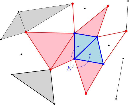
Figure 2: The star of a subcomplex $K^{\prime}\subset K$ is the subcomplex $\operatorname{star}(K^{\prime})\subset K$ that consists all the simplices that share a face with $K^{\prime}$ (this includes all of $K^{\prime}$ itself), and all the faces of these simplices. Here we show an embedded $2$-complex, with all $2$-simplices shaded. The subcomplex $K^{\prime}$ consists of the two indicated triangles, and their faces (blue). The simplices of $\operatorname{star}(K^{\prime})$ are shown in bold (red and blue). The other simplices do not belong to $\operatorname{star}(K^{\prime})$ (black).

A triangulation of $\mathsf{P}\subset\mathbb{R}^{m}$ is an embedded complex $K$ with vertices $\mathsf{P}$ such that $\left|K\right|=\operatorname{conv}(\mathsf{P})$. A complex $K$ is a $j$-manifold complex if the star of every vertex is isomorphic to the star of a triangulation of $\mathbb{R}^{j}$. In order to exploit the local nature of the definition of a manifold complex, it is convenient to have a local notion of triangulation for the star of a vertex in $K$, even if the whole of $K$ is not a triangulation of its vertices:

Definition 2.5 (Triangulation at a point).

A complex $K$ is a triangulation at $p\in\mathbb{R}^{m}$ if:

1. $p$ is a vertex of $K$.

2. $\operatorname{star}(p)$ is embedded.

3. $p$ lies in $\operatorname{int}{\left|\operatorname{star}(p)\right|}$.

4. For all $\tau\in K$, and $\sigma\in\operatorname{star}(p)$, if $(\operatorname{int}{\tau})\cap\sigma\neq\emptyset$, then $\tau\in\operatorname{star}(p)$.

In a general complex Condition 4 above is not a local property, however in the case of Delaunay complexes that intersts us here, local conditions are sufficient to verify the condition, as we will show in Section 3.2.1. Observe also that Condition 4 also precludes intersections with degenerate simplices, since such a simplex would have a face that violates the conditon.

If $\sigma$ is a simplex with vertices in $\mathsf{P}$, then any map $\zeta:\mathsf{P}\to\tilde{\mathsf{P}}\subset\mathbb{R}^{m}$ defines a simplex $\zeta(\sigma)$ whose verticies in $\tilde{\mathsf{P}}$ are the images of vertices of $\sigma$. If $K$ is a complex on $\mathsf{P}$, and $\tilde{K}$ is a complex on $\tilde{\mathsf{P}}$, then $\zeta$ induces a simplicial map $K\to\tilde{K}$ if $\zeta(\sigma)\in\tilde{K}$ for every $\sigma\in K$. We denote this map by the same symbol, $\zeta$. We are interested in the case when $\zeta$ is an isomorphism, which means it establishes a bijection between $K$ and $\tilde{K}$. We then say that $K$ and $\tilde{K}$ are isomorphic, and write $K\cong\tilde{K}$, or $K\overset{\zeta}{\cong}\tilde{K}$ if we wish to emphasise that the correspondence is given by $\zeta$.

A simplicial map $\zeta:K\to\tilde{K}$ defines a continuous map $\zeta:\left|K\right|\to\left|\tilde{K}\right|$, by barycentric interpolation on each simplex $\sigma\in K$. We observe the following consequence of Brouwer’s invariance of domain:

Lemma 2.6.

Suppose $K$ is a complex with vertices $\mathsf{P}\subset\mathbb{R}^{m}$, and $\tilde{K}$ a complex with vertices $\tilde{\mathsf{P}}\subset\mathbb{R}^{m}$. Suppose also that $K$ is a triangulation at $p\in\mathsf{P}$, and that $\zeta:\mathsf{P}\to\tilde{\mathsf{P}}$ induces an injective simplicial map $\operatorname{star}(p)\to\operatorname{star}(\zeta(p))$. If $\operatorname{star}(\zeta(p))$ is embedded, then

$$\zeta(\operatorname{star}(p))=\operatorname{star}(\zeta(p)),$$

and $\zeta(p)$ is an interior point of $\tilde{\mathsf{P}}$.

Proof.

We need to show that $\operatorname{star}(\zeta(p))\subseteq\zeta(\operatorname{star}(p))$. Since $\operatorname{star}(p)$ is embedded, $\zeta$ defines a continuous map $\zeta:\left|\operatorname{star}(p)\right|\to\left|\operatorname{star}(\zeta(p))\right|$ that is injective on each simplex. Since $\operatorname{star}(\zeta(p))$ is also embedded, this continuous map is injective on $\left|\operatorname{star}(p)\right|$. Since $K$ is a triangulation at $p$, there is an open ball $B$ centred at $p$ such that $B\subset\operatorname{int}{\left|\operatorname{star}(p)\right|}$. Then $\zeta|_{B}:\mathbb{R}^{m}\supset B\to\zeta(B)\subset\mathbb{R}^{m}$ is a homeomorphism by Brouwer’s invariance of domain [Dug66, Ch. XVII]. It follows that $\zeta(p)$ is an interior point of $\tilde{\mathsf{P}}$.

Suppose $\sigma\in\operatorname{star}(\zeta(p))$ and $\zeta(p)$ is a vertex of $\sigma$. Then, since $\sigma$ is not degenerate, there is a point $x\in\zeta(B)\cap\operatorname{int}{\sigma}$, and from the above argument, $x$ also lies in the interior of some simplex $\tilde{\tau}\in\zeta(\operatorname{star}(p))\subseteq\operatorname{star}(\zeta(p))$. Since $\operatorname{star}(\zeta(p))$ is embedded, $\tilde{\tau}\cap\sigma$ is a face of $\sigma$ and of $\tilde{\tau}$, but since $x$ is in the interior of both simplices, it must be that $\tilde{\tau}=\sigma$. Thus $\sigma\in\zeta(\operatorname{star}(p))$.

If $\sigma\in\operatorname{star}(\zeta(p))$, then there is some $\tau\in\operatorname{star}(\zeta(p))$ such that $\zeta(p)$ is a vertex of $\tau$ and $\sigma\leq\tau$. Since $\tau\in\zeta(\operatorname{star}(p))$, we also have $\sigma\in\zeta(\operatorname{star}(p))$, by the definition of a simplicial map.

3 Parameterized genericity

In this section we examine the Delaunay complex of $\mathsf{P}\subset\mathbb{R}^{m}$, taking the view that poorly-shaped simplices arise from almost degenerate configurations of points. We introduce the concept of a protected Delaunay ball, which leads to a parameterized definition of genericity. We then show that a lower bound on the protection of the maximal simplices yields a lower bound on their thickness.

3.1 The Delaunay complex

An empty ball is one that contains no point from $\mathsf{P}$.

Definition 3.1 (Delaunay complex).

A Delaunay ball is a maximal empty ball. Specifically, $B=B_{\mathbb{R}^{m}}(x;r)$ is a Delaunay ball if any empty ball centred at $x$ is contained in $B$. A simplex $\sigma$ is a Delaunay simplex if there exists some Delaunay ball $B$ such that the vertices of $\sigma$ belong to $\partial{B}\cap\mathsf{P}$. The Delaunay complex is the set of Delaunay simplices, and is denoted $\operatorname{Del}(\mathsf{P})$.

The Delaunay complex has the combinatorial structure of an abstract simplicial complex, but $\operatorname{Del}(\mathsf{P})$ is embedded only when $\mathsf{P}$ satisfies appropriate genericity requirements, as discussed in Section 3.2. Otherwise, $\operatorname{Del}(\mathsf{P})$ contains degenerate simplices. We make here some observations that are not dependent on assumptions of genericity.

Figure 3: Lemma 3.2: If the affine hull of $\sigma$ is not full dimensional, then a Delaunay ball has freedom to expand, and $\sigma$ must be the face of a higher dimensional Delaunay simplex.

The union of the Delaunay simplices is $\operatorname{conv}(\mathsf{P})$. A simplex $\sigma\in\operatorname{Del}(\mathsf{P})$ is a boundary simplex if all its vertices lie on $\partial{\operatorname{conv}(P)}$. We observe

Lemma 3.2 (Maximal simplices).

If $\operatorname{aff}(\mathsf{P})=\mathbb{R}^{m}$, then every Delaunay $j$-simplex, $\sigma$, is a face of a Delaunay simplex $\sigma^{\prime}$ with $\dim\operatorname{aff}(\sigma^{\prime})=m$. In particular, if $j\leq m$, then $\sigma$ is a face of a Delaunay $m$-simplex. If $\sigma$ is not a boundary simplex, and $\dim\operatorname{aff}(\sigma)<m$, then there are at least two Delaunay $(j+1)$-simplices that have $\sigma$ as a face.

Proof.

Suppose $\dim\operatorname{aff}(\sigma)<m$. Let $B=B_{\mathbb{R}^{m}}(c;r)$ be a Delaunay ball for $\sigma$. Let $\ell$ be the line through $c$ and $C(\sigma)$. If $c=C(\sigma)$, let $\ell$ be any line through $c$ and orthogonal to $\operatorname{aff}(\sigma)$. There must be a point $\hat{c}\in\ell$ such that the circumscribing ball for $\sigma$ centred at $\hat{c}$ is not empty. If this were not the case, we would have $\operatorname{aff}(\sigma)=\operatorname{aff}(\mathsf{P})$, and thus $\dim\operatorname{aff}(\mathsf{P})<m$. It follows then (from the continuity of the radius of the circumballs parameterized by $\ell$), that there is a point $c^{\prime}\in[c,\hat{c}]$ that is the centre of a Delaunay ball for a simplex $\sigma^{\prime}$ that has $\sigma$ as a proper face. The first assertion follows.

The second assertion follows from the same argument, and the observation that if $\sigma$ is not on the boundary of $\operatorname{conv}(\mathsf{P})$, then there must be non-empty balls centred on $\ell$ at either side of $c$. If $p\in\mathsf{P}\setminus\operatorname{aff}(\sigma)$ is on the boundary of an empty ball centred at one side of $c$, by the intersection properties of spheres, it cannot be on the boundary of an empty ball centred on the other side of $c$. Thus there must be at least two distinct Delaunay $(k+1)$-simplices that share $\sigma$ as a face.

Lemma 3.2 gives rise to the following observation, which plays an important role in Section 3.3, where we argue that protecting the Delaunay $m$-simplices yields a thickness bound on the simplices.

Lemma 3.3 (Separation).

If $\tau\in\operatorname{Del}(\mathsf{P})$ is a $j$-simplex that is not a boundary simplex, and $q\in\mathsf{P}\setminus\tau$, then there is a Delaunay $m$-simplex $\sigma^{m}$ which has $\tau$ as a face, but does not include $q$.

Proof.

Assume $j<m$, for otherwise there is nothing to prove. If $\sigma={q}*{\tau}$ is not Delaunay, the assertion follows from the first part of Lemma 3.2. Assume $\sigma$ is Delaunay and let $\tilde{\sigma}^{m}$ be a Delaunay $m$-simplex that has $\sigma$ as a face. Thus $\tilde{\sigma}^{m}={q}*{\sigma^{m-1}}$ for some Delaunay $(m-1)$-simplex, $\sigma^{m-1}$. Since $\tau\leq\sigma^{m-1}$ does not belong to the boundary of $\operatorname{conv}(\mathsf{P})$, neither does $\sigma^{m-1}$, so by the second part of Lemma 3.2, there is another Delaunay $m$-simplex $\sigma^{m}$ that has $\sigma^{m-1}$ (and therefore $\tau$) as a face. Since $\sigma^{m}$ is distinct from $\tilde{\sigma}^{m}$, it does not have $q$ as a vertex.

3.1.1 The Delaunay complex in other metrics

We will also consider the Delaunay complex defined with respect to a metric $d$ on $\mathbb{R}^{m}$ which differs from the Euclidean one. Specifically, if $\mathsf{P}\subset U\subset\mathbb{R}^{m}$ and $d:U\times U\to\mathbb{R}$ is a metric, then we define the Delaunay complex $\operatorname{Del}_{d}(\mathsf{P})$ with respect to the metric $d$.

The definitions are exactly analogous to the Euclidean case: A Delaunay ball is a maximal empty ball $B(x;r)$ in the metric $d$. The resulting Delaunay complex $\operatorname{Del}_{d}(\mathsf{P})$ consists of all the simplices which are circumscribed by a Delaunay ball with respect to the metric $d$. The simplices of $\operatorname{Del}_{d}(\mathsf{P})$ are, possibly degenerate, geometric simplices in $\mathbb{R}^{m}$. As for $\operatorname{Del}(\mathsf{P})$, $\operatorname{Del}_{d}(\mathsf{P})$ has the combinatorial structure of an abstract simplicial complex, but unlike $\operatorname{Del}(\mathsf{P})$, $\operatorname{Del}_{d}(\mathsf{P})$ may fail to be embedded even when there are no degenerate simplices.

3.2 Protection

A Delaunay simplex $\sigma$ is $\delta$-protected if it has a Delaunay ball $B$ such that $d_{\mathbb{R}^{m}}(q,\partial{B})>\delta$ for all $q\in\mathsf{P}\setminus\sigma$. We say that $B$ is a $\delta$-protected Delaunay ball for $\sigma$. If $\tau<\sigma$, then $B$ is also a Delaunay ball for $\tau$, but it cannot be a $\delta$-protected Delaunay ball for $\tau$. We say that $\sigma$ is protected to mean that it is $\delta$-protected for some unspecified $\delta\geq 0$.

Figure 4: A Delaunay simplex $\sigma$ is $\delta$-protected if it has a Delaunay ball $B_{\mathbb{R}^{m}}(c;r)$ such that $\overline{B}_{\mathbb{R}^{m}}(c;r+\delta)\cap(\mathsf{P}\setminus\sigma)=\emptyset$.

Definition 3.4 ($\delta$-generic).

A finite set of points $\mathsf{P}\subset\mathbb{R}^{m}$ is $\delta$-generic if $\operatorname{aff}(\mathsf{P})=\mathbb{R}^{m}$, and all the Delaunay $m$-simplices are $\delta$-protected. The set $\mathsf{P}$ is simply generic if it is $\delta$-generic for some unspecified $\delta\geq 0$.

Observe that we have employed a strict inequality in the definition of $\delta$-protection. In particular, a $\delta$-generic point set is generic even when $\delta=0$. In order for the quantity $\delta$ to be meaningful, it should be considered with respect to a sampling radius $\epsilon$ for $\mathsf{P}$. We will always assume that $\delta\leq\epsilon$.

In his seminal work, Delaunay [Del34] demonstrated that if there is no empty ball with $m+2$ points from $\mathsf{P}$ on its boundary, then $\operatorname{Del}(\mathsf{P})$ is realized as a simplicial complex in $\mathbb{R}^{m}$. In other words $\operatorname{Del}(\mathsf{P})$ is an embedded complex, and in fact it is a triangulation of $\mathsf{P}$, the Delaunay triangulation. If $\mathsf{P}$ is generic according to Definition 3.4, then Delaunay’s criterion will be met. This is obvious if there are no degenerate $m$-simplices, and Definition 3.4 ensures that a degenerate $m$-simplex cannot exist in $\operatorname{Del}(\mathsf{P})$, as shown by Lemma 3.5 below.

In particular, if $\mathsf{P}$ is generic if and only if there are no Delaunay simplices with dimension higher than $m$. We can say more. There are no degenerate Delaunay simplices. This can be inferred directly from Delaunay’s result [Del34], but is also easily established from Lemma 3.2. In Section 3.3 we will quantify this observation with a bound on the thickness of the Delaunay simplices.

The $\delta$-generic assumption means that all the Delaunay $m$-simplices are $\delta$-protected, but the lower dimensional Delaunay do not necessarily enjoy this level of protection. The fact that there are no degenerate Delaunay simplices implies that all the simplices of all dimensions are $\tilde{\delta}$-protected for some $\tilde{\delta}>0$.

3.2.1 Local Delaunay triangulation

Delaunay avoided boundary complications by assuming a periodic point set, but we are particularly interested in the case where the point sets come from local patches of a well-sampled compact manifold without boundary. Periodic boundary conditions are not appropriate in this setting, but this is not a problem because, as we show here, Delaunay’s argument applies locally.

Delaunay’s proof that the Delaunay complex of a generic periodic point set is a triangulation of $\mathbb{R}^{m}$ consists of two observations. First it is observed that if two Delaunay simplices intersect, then they intersect in a common face. This shows that $\operatorname{Del}(\mathsf{P})$ is embedded. The argument is not complicated by the presence of boundary points:

Lemma 3.5 (Embedded star).

Suppose $\operatorname{aff}(\mathsf{P})=\mathbb{R}^{m}$ and $p\in\mathsf{P}$. If all the $m$-simplices in $\operatorname{star}(p;\operatorname{Del}(\mathsf{P}))$ are protected, then $\operatorname{star}(p;\operatorname{Del}(\mathsf{P}))$ is embedded, and it is a pure $m$-complex.

Proof.

We first observe that the $m$-simplices in $\operatorname{star}(p)$ are not degenerate. If $\sigma^{m}$ is degenerate, then by Lemma 3.2, there is a simplex $\tau$ with $\operatorname{aff}(\tau)=\mathbb{R}^{m}$, and $\sigma^{m}<\tau$. We have $\tau\in\operatorname{star}(p)$, since $p\in\tau$. An affinely independent set of $m+1$ vertices from $\tau$ defines a non-degenerate $m$-simplex $\tilde{\sigma}^{m}<\tau$, and since its unique circumball is also a Delaunay ball for $\tau$, it cannot be protected, a contradiction.

Now suppose that $\sigma,\tau\in\operatorname{star}(p)$ and $\sigma\cap\tau\neq\emptyset$. We need to show that they intersect in a common face. By Lemma 3.2, we may assume that $\sigma$ and $\tau$ are $m$-simplices. Assume $\sigma\neq\tau$, and let $B_{1}$ and $B_{2}$ be the Delaunay balls for $\sigma$ and $\tau$. Then $\operatorname{aff}(\partial{B_{1}}\cap\partial{B_{2}})$ defines an $(m-1)$-flat, $H$. Since $B_{1}$ and $B_{2}$ are empty balls, $H$ separates the interiors of $\sigma$ and $\tau$, and thus they must intersect in $H$, i.e., at the common face defined by the vertices in $\partial{B_{1}}\cap\partial{B_{2}}$.

The second observation Delaunay made is that, in the case of a periodic (infinite) point set, every $(m-1)$-simplex is the face of two $m$-simplices (Lemma 3.2). The implication here is that $\operatorname{Del}(\mathsf{P})$ cannot have a boundary, and therefore must cover $\mathbb{R}^{m}$. Here we flesh out the argument for our purposes: If an embedded finite complex contains $m$-simplices then its topological boundary must contain $(m-1)$-simplices. We first observe that the topological boundary of an embedded complex is defined by a subcomplex:

Lemma 3.6 (Boundary complex).

If $K$ is an embedded (finite) complex in $\mathbb{R}^{m}$, then the topological boundary of $\left|K\right|\subset\mathbb{R}^{m}$ is defined by a subcomplex: $\partial{\left|K\right|}=\left|\operatorname{bd}(K)\right|$, where the subcomplex $\operatorname{bd}(K)\subset K$ is called the boundary complex of $K$.

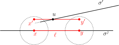
Figure 5: Diagram for the proof of Lemma 3.6.

Proof.

Since $K$ is finite, $\partial{\left|K\right|}$ is contained in $\left|K\right|$. Suppose $x\in\partial{\left|K\right|}$. Then $x\in\operatorname{int}{\sigma^{j}}$ for some $\sigma^{j}\in K$. We wish to show that $\sigma^{j}\subset\partial{\left|K\right|}$. Suppose to the contrary that $y\in\operatorname{int}{\sigma^{j}}$, but $y$ does not belong to $\partial{\left|K\right|}$. This means that $y\in\operatorname{int}{\left|K\right|}$.

Consider the segment $\ell=[x,y]\subset\operatorname{int}{\sigma^{j}}$. Let $Z\subset K$ be the subcomplex consisting of those simplices that do not contain $\sigma^{j}$. Let

$$r_{1}=\min_{\sigma\in Z}d_{\mathbb{R}^{m}}(\ell,\sigma).$$

Choosing $r\leq r_{1}$, and $x^{\prime}\in B_{\mathbb{R}^{m}}(x;r)\setminus\left|K\right|$, let $y^{\prime}=y+(x^{\prime}-x)$. Since $y\in\operatorname{int}{\left|K\right|}$, we may assume that $r$ is small enough so that $y^{\prime}\in\operatorname{int}{\left|K\right|}$.

Consider the segment $\ell^{\prime}=[x^{\prime},y^{\prime}]$. By construction, $\ell^{\prime}\cap\left|Z\right|=\emptyset$. However, consider the point $u\in\operatorname{int}{\ell^{\prime}}$ that is the point in $\ell^{\prime}\cap\left|K\right|$ that is closest to $x^{\prime}$. The point $u$ lies in the interior of some simplex $\sigma^{\prime}\in K$, but we cannot have $\sigma^{j}\leq\sigma^{\prime}$. Indeed if this were the case, $x^{\prime}$ would lie in $\operatorname{aff}(\sigma^{\prime})$, and so $u\in\partial{\sigma^{\prime}}$, contradicting the assumption that $u\in\operatorname{int}{\sigma^{\prime}}$.

But this means that $\sigma^{\prime}\in Z$, which contradicts the fact that $\ell^{\prime}\cap\left|Z\right|=\emptyset$. Therefore we must have $y\in\partial{\left|K\right|}$ for all $y\in\operatorname{int}{\sigma^{j}}$.

Finally, observe that if $\tau<\sigma^{j}$, then $\tau\subset\partial{\left|K\right|}$, since $\partial{\left|K\right|}$ is closed.

Lemma 3.7 (Pure boundary complex).

If $K$ is a (finite) pure $m$-complex embedded in $\mathbb{R}^{m}$, then its boundary complex is a pure $(m-1)$-complex.

Figure 6: Diagram for the proof of Lemma 3.7.

Proof.

Since $K$ is finite, $\operatorname{bd}(K)$ is nonempty; it contains at least the vertices in $\partial{\operatorname{conv}(\left|K\right|)}$. We will show that if $\sigma^{j}\in\operatorname{bd}(K)$, is a $j$-simplex, with $0\leq j<m-1$, then there is a $\sigma^{k}\in\operatorname{bd}(K)$ with $\sigma^{j}<\sigma^{k}$. The result then follows, since $\operatorname{bd}(K)$ cannot contain $m$-simplices, because $K$ is embedded.

Suppose $\sigma^{j}\in\operatorname{bd}(K)$, and $x\in\operatorname{int}{\sigma^{j}}$. Let $Z\subset K$ be the subcomplex consisting of simplices that do not contain $\sigma^{j}$, and let

$$r=\min_{\sigma\in Z}d_{\mathbb{R}^{m}}(x,\sigma).$$

Let $B=B_{\mathbb{R}^{m}}(x;r)$, and choose $y\in B\setminus\left|K\right|$. Let $F$ be the $(m-j)$-dimensional affine space orthogonal to $\operatorname{aff}(\sigma^{j})$ and containing $y$, and let $S^{m-j-1}=F\cap\partial{B_{\mathbb{R}^{m}}(x;r^{\prime})}$, where $r^{\prime}=\left\|x-y\right\|$. See Figure 6.

Since $K$ is pure, there is an $m$-simplex $\sigma^{m}$ with $\sigma^{j}<\sigma^{m}$. We have $\sigma^{m}\cap S^{m-j-1}\neq\emptyset$. Indeed, choose $w\in\operatorname{int}{\sigma^{m}}$, and $u\in\sigma^{j}$ different from $x$, and observe that the plane $Q$ defined by $x,w,u$ intersects $B\cap\sigma^{m}$ in a semi-disk, by construction of $B$. By the construction of $S^{m-j-1}$, it must intersect this semidisk.

Let $z\in S^{m-j-1}$ be a point that minimises the geodesic distance in $S^{m-j-1}$ to $y$. Then $z\in\partial{\left|K\right|}$. Thus $z\in\operatorname{int}{\sigma^{k}}$ for some $\sigma^{k}\in\operatorname{bd}(K)$, and since $z\in B$, $\sigma^{k}$ cannot belong to $Z$. Thus $\sigma^{j}\leq\sigma^{k}$, but since $S^{m-j-1}\cap\sigma^{j}=\emptyset$, we have $\sigma^{j}<\sigma^{k}$.

From Lemma 3.2, Lemma 3.5, and Lemma 3.7, one can verify that if $\mathsf{P}$ is generic then $\partial{\operatorname{conv}(\mathsf{P})}=\partial{\left|\operatorname{Del}(\mathsf{P})\right|}$, and thus obtain the standard result that $\operatorname{Del}(\mathsf{P})$ is a triangulation of $\mathsf{P}$. However, we are interested localizing the result, without the assumption that the entire point set is generic. We have the following local version of Delaunay’s triangulation result:

Lemma 3.8 (Local Delaunay triangulation).

If $p\in\mathsf{P}$ is an interior point, and the Delaunay $m$-simplices incident to $p$ are protected, then $\operatorname{Del}(\mathsf{P})$ is a triangulation at $p$.

Proof.

By Lemma 3.5, $\operatorname{star}(p)$ is a pure $m$-complex, and it is embedded. It follows then from Lemma 3.7, that the boundary complex $\operatorname{bd}(\operatorname{star}(p))$ is a pure $(m-1)$-complex. Thus $p$ cannot belong to $\operatorname{bd}(\operatorname{star}(p))$. Indeed, it follows from Lemma 3.2 that any $(m-1)$-simplex $\sigma\in\operatorname{star}(p)$ is the face of at least two $m$-simplices in $\operatorname{Del}(\mathsf{P})$, and if $p\in\sigma$, then both of these $m$-simplices belong to $\operatorname{star}(p)$, and are embedded, with intersection $\sigma$. Thus $p$ cannot belong to an $(m-1)$-simplex in $\operatorname{bd}(\operatorname{star}(p))$, and therefore $p\in\operatorname{int}{\left|\operatorname{star}(p)\right|}$.

It remains to verify Condition 4 of Definition 2.5. The argument is similar to the proof of Lemma 3.5: Suppose $x\in(\operatorname{int}{\tau})\cap\sigma$ for $\sigma\in\operatorname{star}(p)$. We may assume that $\sigma$ is an $m$-simplex. Then consider the Delaunay balls $B_{1}$ for $\sigma$ and $B_{2}$ for $\tau$. If $B_{1}=B_{2}$, then, since $\sigma$ is protected, $\tau$ must be a face of $\sigma$, and so belong to $\operatorname{star}(p)$. Assume then that $B_{1}\neq B_{2}$, and let $H$ be the $(m-1)$-flat defined by $\operatorname{aff}(\partial{B_{1}}\cap\partial{B_{2}})$. Since $B_{1}$ is empty, $x\in\operatorname{int}{\tau}$ cannot lie in the open half-space defined by $H$ and containing $\sigma$. Since $x\in\sigma$ also, it must lie in $H$, and therefore all vertices of $\tau$ lie in $H\cap\partial{B_{2}}=H\cap\partial{B_{1}}$, and so $\tau$ is a face of $\sigma$.

3.2.2 Safe interior simplices

We wish to consider the properties of Delaunay triangulations in regions which are comfortably in the interior of $\operatorname{conv}(\mathsf{P})$, and avoid the complications that arise as we approach the boundary of the point set. We introduce some terminology to facilitate this.

If none of the vertices of $\sigma$ lie on $\partial{\operatorname{conv}(P)}$, then it is an interior simplex. We wish to identify a subcomplex of the interior simplices of $\operatorname{Del}(\mathsf{P})$ consisting of those simplices whose neighbour simplices are also all interior simplices with small circumradius. An interior simplex near the boundary of $\operatorname{conv}(\mathsf{P})$ does not necessarily have its circumradius constrained by the sampling radius. However, we have the following:

Lemma 3.9.

If $\mathsf{P}$ is an $\epsilon$-sample set, and $\sigma\in\operatorname{Del}(\mathsf{P})$ has a vertex $p$ such that $d_{\mathbb{R}^{m}}(p,\partial{\operatorname{conv}(\mathsf{P})})\geq 2\epsilon$, then $R(\sigma)<\epsilon$ and $\sigma$ is an interior simplex.

Proof.

Let $B_{\mathbb{R}^{m}}(c;r)$ be a Delaunay ball for $\sigma$. We will show $r<\epsilon$. Suppose to the contrary. Let $x$ be the point on $[c,p]$ such that $d_{\mathbb{R}^{m}}(p,x)=\epsilon$. Then $p$ is the closest point in $\mathsf{P}$ to $x$, and so the sampling criteria imply that $d_{\mathbb{R}^{m}}(x,\partial{\operatorname{conv}(\mathsf{P})})<\epsilon$. But then $d_{\mathbb{R}^{m}}(p,\partial{\operatorname{conv}(\mathsf{P})})\leq d_{\mathbb{R}^{m}}(p,x)+d_{\mathbb{R}^{m}}(x,\partial{\operatorname{conv}(\mathsf{P})})<2\epsilon$, contradicting the hypothesis on $p$.

Thus $r<\epsilon$, and it follows that $\sigma$ is an interior simplex because if $q\in\sigma$, then $d_{\mathbb{R}^{m}}(p,q)\leq 2r<d_{\mathbb{R}^{m}}(p,\partial{\operatorname{conv}(\mathsf{P})})$.

This suggests the following:

Definition 3.10 (Deep interior points).

Suppose $\mathsf{P}\subset\mathbb{R}^{m}$ is an $\epsilon$-sample set. The subset $\mathsf{P}_{I}\subset\mathsf{P}$ consisting of all $p\in\mathsf{P}$ with $d_{\mathbb{R}^{m}}(p,\partial{\operatorname{conv}(\mathsf{P})})\geq 4\epsilon$ is the set of deep interior points.

By Lemma 3.9, all the simplices that include a deep interior point, as well as all the neighbours of such simplices, will have a small circumradius. For technical reasons it is inconvenient to demand that all the Delaunay $m$-simplices be $\delta$-protected. We focus instead on a subset defined with respect to a set of deep interior points:

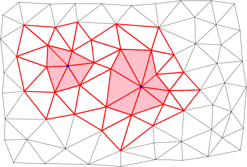
Figure 7: If $\mathsf{P}$ is $\delta$-generic for $\mathsf{P}_{J}$, then the safe interior simplices are the simplices in $\operatorname{star}(\mathsf{P}_{J})$. Here $\mathsf{P}_{J}$ consists of the two large vertices (blue). They must be at least $4\epsilon$ from $\partial{\operatorname{conv}(\mathsf{P})}$ (which is not depicted in the figure). The safe interior simplices are shaded. All the simplices in $\operatorname{star}(\operatorname{star}(\mathsf{P}_{J}))$ are $\delta$-protected. These simplices have bold outlines (red), but are not necessarily shaded.

Definition 3.11 ($\delta$-generic for $\mathsf{P}_{J}$).

The set $\mathsf{P}\subset\mathbb{R}^{m}$ is $\delta$-generic for $\mathsf{P}_{J}$ if $\mathsf{P}_{J}\subseteq\mathsf{P}_{I}$ and all the $m$-simplices in $\operatorname{star}(\operatorname{star}(\mathsf{P}_{J};\operatorname{Del}(\mathsf{P})))$ are $\delta$-protected. The safe interior simplices are the simplices in $\operatorname{star}(\mathsf{P}_{J};\operatorname{Del}(\mathsf{P}))$.

Thus the safe interior simplices are determined by our choice of $\mathsf{P}_{J}\subseteq\mathsf{P}_{I}$, and our protection requirements ensure that all the $m$-simplices that share a face with a safe interior simplex are $\delta$-protected and have a small circumradius. A schematic example is depicted in Figure 7.

3.3 Thickness from protection

Our goal here is to demonstrate that the safe interior simplices on a $\delta$-generic point set are $\Upsilon_{0}$-thick. If $\delta=\nu_{0}\epsilon$, for some constant $\nu_{0}\leq 1$, then we obtain a constant $\Upsilon_{0}$ which depends only on $\nu_{0}$. The key observation is that together with Lemma 3.3, protection imposes constraints on all the Delaunay simplices; they cannot be too close to being degenerate. In the particular case that $j=0$, Lemma 3.3 immediately implies that the vertices of the safe interior simplices are $\delta$-separated:

Lemma 3.12 (Separation from protection).

If $\mathsf{P}$ is $\delta$-generic for $\mathsf{P}_{J}$, then $L(\sigma)>\delta$ for any safe interior simplex $\sigma$.

(a) $H$ separates $c$ and $q$

(b) $q$ and $c$ on same side of $H$

Figure 8: Diagram for Lemma 3.13. LABEL:sub@sfig:opposite.centres When $H$ separates $q$ and $c$ then $d_{\mathbb{R}^{d}}(q,q^{*})>\delta$. LABEL:sub@sfig:q.with.centre Otherwise, a lower bound on the distance between $q$ and its projection $q^{*}$ on $H$ is obtained by an upper bound on the angle $\angle qab$.

Lemma 3.13.

Suppose that $B=B_{\mathbb{R}^{m}}(c;r)$ is a Delaunay ball for $\sigma={q}*{\tau}$ with $r<\epsilon$ and that $L(\tau)\geq\lambda$ for some $\lambda\leq\epsilon$. Suppose also that $\tau\leq\sigma^{\prime}$ and that $\sigma$ is not a face of $\sigma^{\prime}$.

If $B^{\prime}$ is a $\delta$-protected Delaunay ball for $\sigma^{\prime}$, and $H=\operatorname{aff}(\partial{B}\cap\partial{B^{\prime}})$, then

$$d_{\mathbb{R}^{m}}(q,H)>\frac{\sqrt{3}\delta}{4\epsilon}(\lambda+\delta).$$

It follows that, if $\mathsf{P}$ is $\delta$-generic for $\mathsf{P}_{J}$, with sampling radius $\epsilon$, and $\tau$ is a safe interior simplex, then

$$D(q,\sigma)>\frac{\sqrt{3}\delta^{2}}{2\epsilon}.$$

Proof.

Let $B^{\prime}=B_{\mathbb{R}^{m}}(c^{\prime};r^{\prime})$ be the $\delta$-protected Delaunay ball for $\sigma^{\prime}$. Our geometry will be performed in the plane, $Q$, defined by $c$, $c^{\prime}$, and $q$. This plane is orthogonal to the $(m-1)$-flat $H$, and it follows that the distance $d_{\mathbb{R}^{m}}(q,H)$ is realized by a segment in the plane $Q$: the projection, $q^{*}$, of $q$ onto $H$ lies in $Q$, and $d_{\mathbb{R}^{m}}(q,H)=d_{\mathbb{R}^{m}}(q,q^{*})$.

If $H$ separates $q$ from $c$, then $\partial{B^{\prime}}$ separates $q$ from $q^{*}$, and $d_{\mathbb{R}^{m}}(q,q^{*})>d_{\mathbb{R}^{m}}(q,\partial{B^{\prime}})>\delta$, since $B^{\prime}$ is $\delta$-protected (Figure 8LABEL:sub@sfig:opposite.centres). The lemma then follows since $\lambda$ and $\delta$ are each no larger than $\epsilon$. Thus assume that $q$ and $c$ lie on the same side of $H$, as shown in Figure 8LABEL:sub@sfig:q.with.centre. Let $S^{\prime}=Q\cap\partial{B^{\prime}}$, and $S=Q\cap\partial{B}$, and let $a$ and $b$ be the points of intersection $S^{\prime}\cap S$. Thus $H\cap Q$ is the line through $a$ and $b$.

We will bound $d_{\mathbb{R}^{m}}(q,q^{*})$ by finding an upper bound on the angle $\gamma=\angle qab$. This is the same as the standard calculation for upper-bounding the angles in a triangle with bounded circumradius to shortest edge ratio. Without loss of generality, we may assume that $\gamma\geq\angle qba$, and we will assume that $\gamma\geq\pi/2$ since otherwise $q*\in B^{\prime}$ and thus $d_{\mathbb{R}^{m}}(q,q*)>\delta$ and the lemma is again trivially satisified.

Since $d_{\mathbb{R}^{m}}(a,q)>\delta$, we have $d_{\mathbb{R}^{m}}(q,q^{*})=d_{\mathbb{R}^{m}}(a,q)\sin\gamma>\delta\sin\gamma$. Also note that $d(a,b)\geq 2R(\tau)\geq L(\tau)\geq\lambda$. Let $\alpha=\angle qac$. Then $\cos\alpha=\frac{d_{\mathbb{R}^{m}}(a,q)}{2r}\geq\frac{\delta}{2\epsilon}$, which means that $\alpha\leq\arccos\frac{\delta}{2\epsilon}\leq\frac{\pi}{2}$. Similarly, with $\beta=\angle cab$, we have $\beta\leq\arccos\frac{\lambda}{2\epsilon}\leq\frac{\pi}{2}$. Thus $\frac{\pi}{2}\leq\gamma=\alpha+\beta\leq\gamma^{\prime}$, where

$$\gamma^{\prime}=\arccos\frac{\delta}{2\epsilon}+\arccos\frac{\lambda}{2\epsilon}.$$

Since $\sin\gamma\geq\sin\gamma^{\prime}$, when $\frac{\pi}{2}\leq\gamma\leq\gamma^{\prime}\leq\pi$, we have

$$\begin{split}d_{\mathbb{R}^{m}}(q,q^{*})&>\delta\sin\gamma\geq\delta\sin\gamma^{\prime}\\ &=\delta\sin\left(\arccos\frac{\delta}{2\epsilon}+\arccos\frac{\lambda}{2\epsilon}\right)\\ &\geq\delta\left(\frac{\lambda}{2\epsilon}\sin\left(\arccos\frac{\delta}{2\epsilon}\right)+\frac{\delta}{2\epsilon}\sin\left(\arccos\frac{\lambda}{2\epsilon}\right)\right)\\ &\geq\frac{\sqrt{3}\delta}{4\epsilon}(\lambda+\delta),\end{split}$$

where the last inequality follows from $\lambda\leq\epsilon$ and $\delta\leq\epsilon$.

Since $\operatorname{aff}(\tau)\subset H$, it follows that $D(q,\sigma)\geq d_{\mathbb{R}^{m}}(q,H)$, and if $\mathsf{P}$ is $\delta$-generic for $\mathsf{P}_{J}$, then $\lambda\geq\delta$, and Lemma 3.3 ensures that there is a $\delta$-protected $\sigma^{\prime}$ that contains $\tau$ but not $q$.

We thus obtain a bound on the thickness of the safe interior simplices when $\mathsf{P}$ is $\delta$-generic for $\mathsf{P}_{J}$. Since Lemma 3.13 yields a lower bound of $\frac{\sqrt{3}\delta^{2}}{2\epsilon}$ on the altitudes of the safe interior simplices, and since $\Delta(\sigma)\leq 2\epsilon$, we have that $\Upsilon(\sigma)\geq\frac{\sqrt{3}\delta^{2}m}{4\epsilon^{2}}$ for all safe interior $\sigma$. If $\delta=\nu_{0}\epsilon$, we obtain a constant thickness bound.

Theorem 3.14 (Thickness from protection).

If $\mathsf{P}\subset\mathbb{R}^{m}$ is $\delta$-generic for $\mathsf{P}_{J}$ with $\delta=\nu_{0}\epsilon$, where $\epsilon$ is a sampling radius for $\mathsf{P}$, then the safe interior simplices are $\Upsilon_{0}$-thick, with

$$\Upsilon_{0}=\frac{\sqrt{3}\nu_{0}^{2}}{4m}.$$

4 Delaunay stability

We find upper bounds on the magnitude of a perturbation for which a protected Delaunay ball remains a Delaunay ball. We consider both perturbations of the sample points in Euclidean space, and perturbations of the metric itself. The primary technical challenge is bounding the effect of a perturbation on the circumcentre of an $m$-simplex. We then find the relationship between the perturbation parameter $\rho$ and the protection parameter $\delta$ which ensures that a $\delta$-protected Delaunay simplex will remain a Delaunay simplex.

4.1 Perturbations and circumcentres

As expected, a bound on the displacement of the circumcentre requires a bound on the thickness of the simplex.

4.1.1 Almost circumcentres

If $\sigma$ is thick, a point whose distances to the vertices of $\sigma$ are all almost the same, will lie close to $N(\sigma)$.

Lemma 4.1.

If $\sigma=[p_{0},...,p_{k}]\subset\mathbb{R}^{m}$ is a non-degenerate $k$-simplex, and $x\in\mathbb{R}^{m}$ is such that

$$\left|\left\|p_{i}-x\right\|^{2}-\left\|p_{j}-x\right\|^{2}\right|\leq\xi^{2}\quad\text{ for all }i,j\in[0,...,k],$$ (2)

then there is a point $c\in N(\sigma)$ such that $\left\|c-x\right\|\leq\eta$, where

$$\eta=\frac{\xi^{2}}{2\Upsilon(\sigma)\Delta(\sigma)}.$$

In particular, if $\sigma$ is an $m$-simplex then $x\in\overline{B}_{\mathbb{R}^{m}}(C(\sigma);\eta)$.

If the inequalities in Equations (2) are made strict, then the conclusions may also be stated with strict inequalities.

Proof.

First suppose $k=m$. The circumcentre of $\sigma$ is given by the linear equations $\left\|C(\sigma)-p_{i}\right\|^{2}=\left\|C(\sigma)-p_{0}\right\|^{2}$, or

$${(p_{i}-p_{0})}^{\mathsf{T}}C(\sigma)=\frac{1}{2}(\left\|p_{i}\right\|^{2}-\left\|p_{0}\right\|^{2}).$$

Letting $b$ be the vector whose $i^{\text{th}}$ component is defined by the right hand side of the equation, and letting $P$ be the $m\times m$ matrix, whose $i^{\text{th}}$ column is $(p_{i}-p_{0})$, we write the equations in matrix form:

$${P}^{\mathsf{T}}C(\sigma)=b.$$ (3)

Without loss of generality, assume $p_{0}$ is the vertex that minimizes the distance to $x$. Then, defining $x_{a}$ to be the vector whose $i^{\text{th}}$ component is $\frac{1}{2}(\left\|p_{i}-x\right\|^{2}-\left\|p_{0}-x\right\|^{2})$, we have $\left\|p_{i}-x\right\|^{2}=\left\|p_{0}-x\right\|^{2}+2(x_{a})_{i}$, and we find

$${P}^{\mathsf{T}}x=b-x_{a}.$$ (4)

From Equations (3) and (4) we have

$$\left\|C(\sigma)-x\right\|=\left\|{({P}^{\mathsf{T}})}^{-1}x_{a}\right\|\leq\left\|{P}^{-1}\right\|\left\|x_{a}\right\|.$$

From Equation (2), it follows that $\left\|x_{a}\right\|\leq\frac{\sqrt{m}\xi^{2}}{2}$, and from Lemmas 2.3 and 2.4 we have $\left\|{P}^{-1}\right\|\leq(\sqrt{m}\Upsilon(\sigma)\Delta(\sigma))^{-1}$, and thus the result holds for full dimensional simplices.

If $\sigma$ is a $k$-simplex with $k\leq m$, then we consider $\hat{x}$, the orthogonal projection of $x$ into $\operatorname{aff}(\sigma)$. We observe that $\hat{x}$ also must satisfy Equation (2), and we conclude from the above argument that $\left\|C(\sigma)-\hat{x}\right\|\leq\eta$. Then letting $c=C(\sigma)+(x-\hat{x})$ we have that $c\in N(\sigma)$ and $\left\|c-x\right\|\leq\eta$.

It will be convenient to have a name for a point that is almost equidistant to the vertices of a simplex:

Definition 4.2.

A $\xi$-centre for a simplex $\sigma=[p_{0},\ldots,p_{k}]\subset\mathbb{R}^{m}$ is a point $x$ that satisfies

$$\big{|}\left\|p_{i}-x\right\|-\left\|p_{j}-x\right\|\big{|}\leq\xi\qquad\text{ for all }i,j\leq k.$$ (5)

With a bound on the distance from $x$ to the vertices of $\sigma$, Lemma 4.1 can be transformed into a bound on the distance from a $\xi$-centre to the closest true centre in $N(\sigma)$:

Lemma 4.3.

If $\sigma=[p_{0},\ldots,p_{k}]\subset\mathbb{R}^{m}$ is non-degenerate, and for some $\xi>0$ the point $x\in\mathbb{R}^{m}$ is a $\xi$-centre such that

$$\left\|p_{i}-x\right\|<\tilde{\epsilon}\qquad\text{ for all }i,j\leq k,$$

then there exists a $c\in N(\sigma)$ such that $\left\|x-c\right\|<\eta$, where

$$\eta=\frac{\tilde{\epsilon}\xi}{\Upsilon(\sigma)\Delta(\sigma)}.$$

In particular, if $\sigma$ is an $m$-simplex, then $x\in B_{\mathbb{R}^{m}}(C(\sigma);\eta)$.

Proof.

Let $R=\max_{i}\left\|p_{i}-x\right\|$ and $r=\min_{i}\left\|p_{i}-x\right\|$. Then

$$R^{2}-r^{2}=(R+r)(R-r)<2\tilde{\epsilon}(R-r)\leq 2\tilde{\epsilon}\xi,$$

and the result then follows from Lemma 4.1.

4.1.2 Circumcentres and metric perturbations

We will show here that for an $\Upsilon_{0}$-thick $m$-simplex $\sigma$ in $\mathbb{R}^{m}$, and a metric $d$ that is close to $d_{\mathbb{R}^{m}}$, there will be a metric circumcentre $c$ near $C(\sigma)$. We require the metric $d$ to be continuous in the topology defined by $d_{\mathbb{R}^{m}}$. Henceforth, whenever we refer to a perturbation of the Euclidean metric, this topological compatibility will always be assumed.

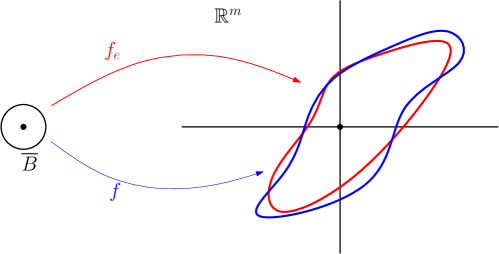
Figure 9: The maps $f_{e}$ and $f$ (described in the main text) map circumcentres to the origin. Since $f_{e}^{-1}(0)$ contains a unique point, and $f_{e}(\partial{B})$ lies far from the origin, a consideration of the degree of the mappings, together with the fact that $f_{e}(\partial{B})$ and $f(\partial{B})$ are close, reveals that $f^{-1}(0)$ cannot be empty, and thus $B$ must contain a circumcentre of $\sigma^{m}$ with respect to the metric $d$.

The proof is a topological argument based on considering a mapping into $\mathbb{R}^{m}$ of a small ball around the circumcentre of $\sigma$. The mapping is based on the metric and is such that circumcentres get mapped to the origin. In the mapping associated to the Euclidean metric, points that get mapped close to the origin are $\xi$-centres, and since the $\xi$-centres are in the interior of the ball, the boundary of the ball does not get mapped close to the origin. A small perturbation of the metric yields a small perturbation in the mapping, and so we can argue that there is a homotopy between the mapping associated with the Euclidean metric and the one associated to the perturbed metric, such that no point on the boundary of the ball ever gets mapped to the origin. The situation is depicted schematically in Figure 9. A consideration of the degree of the mapping allows us to conclude that the ball must contain a circumcentre for the perturbed metric.

We will demonstrate the following:

Lemma 4.4 (Circumcentres: metric perturbation).

Let $U\subset\mathbb{R}^{m}$, and let $d:U\times U\to\mathbb{R}$ be a continuous metric with respect to the topology defined by $d_{\mathbb{R}^{m}}$, and such that for any $x,y\in U$ with $d_{\mathbb{R}^{m}}(x,y)<2\epsilon$, we have $\left|d(x,y)-d_{\mathbb{R}^{m}}(x,y)\right|\leq\rho$, with

$$\rho\leq\frac{\Upsilon_{0}\mu_{0}\epsilon}{8}.$$

If $\sigma=[p_{0},\ldots,p_{m}]\subset U$ is an $\Upsilon_{0}$-thick $m$-simplex with $R(\sigma)<\epsilon$, and $L(\sigma)\geq\mu_{0}\epsilon$, and such that $d_{\mathbb{R}^{m}}(p_{i},\partial{U})\geq 2\epsilon$, then there is a point

$$c\in B=B_{\mathbb{R}^{m}}(C(\sigma);\eta)\quad\text{ with }\eta=\frac{8\rho}{\Upsilon_{0}\mu_{0}},$$

and such that $d(c,p_{i})=d(c,p_{j})$ for all $p_{i},p_{j}\in\sigma$.

In order to prove Lemma 4.4, we will use a particular case of Lemma 4.3:

Lemma 4.5.

Suppose $\sigma$ is an $\Upsilon_{0}$-thick $m$-simplex such that $L(\sigma)\geq\mu_{0}\epsilon$. If $x$ is a $\xi$-centre for $\sigma$ with $d_{\mathbb{R}^{m}}(x,p)<2\epsilon$ for all $p\in\sigma$, then $x\in B_{\mathbb{R}^{m}}(C(\sigma);\eta)$, where $\eta=\frac{2\xi}{\Upsilon_{0}\mu_{0}}$.

Let $B=B_{\mathbb{R}^{m}}(C(\sigma);\eta)$ be the open ball which contains the $\xi$-centres for $\sigma$. We will show that if $\xi=4\rho$, then a circumcentre $c$ for $\sigma$ with respect to $d$ will also lie in $B$. However, we make no claim that $c$ is unique. Note that $\overline{B}\subset U$.

Consider the function $f_{e}:\overline{B}\to\mathbb{R}^{m}$ given by

$$f_{e}(x)={(d_{\mathbb{R}^{m}}(x,p_{1})-d_{\mathbb{R}^{m}}(x,p_{0}),\ldots,d_{\mathbb{R}^{m}}(x,p_{m})-d_{\mathbb{R}^{m}}(x,p_{0}))}^{\mathsf{T}}.$$ (6)

Observe that $f_{e}$ maps the circumcentre of $\sigma$, and only the circumcentre, to the origin: $f_{e}^{-1}(0)=\{C(\sigma)\}$.

We construct a similar function for the metric $d$,

$$f(x)={(d(x,p_{1})-d(x,p_{0}),\ldots,d(x,p_{m})-d(x,p_{0}))}^{\mathsf{T}},$$ (7)

and we will show that there must be a $c\in f^{-1}(0)\subset B$. We first show that there is a homotopy between $f$ and $f_{e}$ such that the image of $\partial{\overline{B}}$ never touches the origin:

Lemma 4.6.

Under the hypotheses of Lemma 4.4, if $\xi=4\rho\leq\frac{\Upsilon_{0}\mu_{0}\epsilon}{2}$, then there is a homotopy $F:\overline{B}\times[0,1]\to\mathbb{R}^{m}$ between $f_{e}(x)=F(x,0)$ and $f(x)=F(x,1)$ with $F(x,t)\neq 0$ for all $x\in\partial{\overline{B}}$ and $t\in[0,1]$.

Proof.

We define the homotopy $F:\overline{B}\times[0,1]\to\mathbb{R}^{m}$ by $F(x,t)=(1-t)f_{e}(x)+tf(x)$. By the bounds on $\xi$ and $R(\sigma)$, for every $x\in\overline{B}$, and $p\in\sigma$, we have $d_{\mathbb{R}^{m}}(x,p)\leq\frac{2\xi}{\Upsilon_{0}\mu_{0}}+R(\sigma)<2\epsilon$. Thus it follows from Lemma 4.5 that $x\in\partial{\overline{B}}$ cannot be a $\xi$-centre.

It is convenient to consider the max norm on $\mathbb{R}^{m}$ defined by the largest magnitude of the components: $\left\|f_{e}(x)\right\|_{\infty}=\max_{i}\left|f_{e}(x)_{i}\right|$. (This gives us a better bound than working with the standard Euclidean norm.) If $\left\|f_{e}(y)\right\|_{\infty}\leq\frac{\xi}{2}$, then $y$ must be a $\xi$-centre. Indeed, we would have $\left|\left\|p_{i}-y\right\|-\left\|p_{j}-y\right\|\right|\leq\left|\left\|p_{i}-y\right\|-\left\|p_{0}-y\right\|\right|+\left|\left\|p_{0}-y\right\|-\left\|p_{j}-y\right\|\right|\leq\frac{\xi}{2}+\frac{\xi}{2}=\xi$ for all $i$ and $j$. Thus, since $x\in\partial{\overline{B}}$ is not a $\xi$-centre, we must have $\left\|f_{e}(x)\right\|_{\infty}>\frac{\xi}{2}$.

Also, from the hypothesis on $d$, we have $\left\|f_{e}(x)-f(x)\right\|_{\infty}\leq 2\rho=\frac{\xi}{2}$, for all $x\in\partial{\overline{B}}$. It follows that $\left\|F(x,t)\right\|_{\infty}\geq\left\|f_{e}(x)\right\|_{\infty}-t\left\|f(x)-f_{e}(x)\right\|_{\infty}>0$ when $x\in\partial{\overline{B}}$.

We will need the following observation:

Lemma 4.7.

The origin is a regular value for the function $f_{e}$ defined in Equation (6).

Proof.

Choose a coordinate system such that $C(\sigma)\in B$ is the origin. We show by a direct calculation that $\det J(f_{e})_{0}\neq 0$, where $J(f_{e})_{0}$ is the Jacobian matrix representing the derivative of $f_{e}$ in our coordinate system.

Let $p_{i}={(p_{i0},\,\dots,\,p_{im})}^{\mathsf{T}}$ for all $p_{i}\in\{p_{0},\,\dots,\,p_{m}\}$. For $x={(x_{1},\,\dots,\,x_{m})}^{\mathsf{T}}\in\mathbb{R}^{m}$, let $f_{e}(x)={(f_{0}(x),\,\dots,\,f_{m}(x))}^{\mathsf{T}}$, where

$$f_{i}(x)=\|p_{i}-x\|-\|p_{0}-x\|=\sqrt{\sum_{k=1}^{m}(p_{ik}-x_{k})^{2}}-\sqrt{\sum_{k=1}^{m}(p_{0k}-x_{k})^{2}}\,.$$

We find

$$\frac{\partial f_{i}}{\partial x_{j}}\Big{|}_{0}=\frac{p_{0j}-p_{ij}}{R(\sigma)},$$

and thus

$$J(f_{e})_{0}=-\frac{1}{R(\sigma)}{P}^{\mathsf{T}},$$ (8)

where as usual $P$ is the matrix whose columns are $p_{i}-p_{0}$. Since $\operatorname{vol}(\sigma^{m})=\frac{|\det(P)|}{m!}$, Equation (8) implies

$$\left|\det J(f_{e})_{0}\right|=\frac{m!\,\operatorname{vol}(\sigma^{m})}{R(\sigma)^{m}}.$$

Thus since $f_{e}^{-1}(0)=\{0\}$, $0$ is a regular value for $f_{e}$ provided $\sigma$ is non-degenerate.

Lemma 4.4 now follows from a consideration of the degree of the mappings $f$ and $f_{e}$ relative to zero. The degree of a smooth map $g:\overline{B}\to\mathbb{R}^{m}$ at a regular point $p\in g(B)$ is defined by

$$\deg(g,p,B)=\sum_{x\in g^{-1}(p)}\operatorname{sign}\det J(g)_{x}\,,$$

where $J(g)_{x}$ is the Jacobian matrix of $g$ at $x$. The exposition by Dancer [Dan00] is a good reference for the degree of maps from manifolds with boundary. It is shown that the definition of $\deg(g,p,B)$ extends to continuous maps $g$ that are not necessarily differentiable. If $h:\overline{B}\to\mathbb{R}^{m}$ is homotopic to $g$ by a homotopy $H:\overline{B}\times[0,1]\to\mathbb{R}^{m}$ such that $H(x,t)\neq p$ for all $t\in[0,1]$, and $x\in\partial{B}$, then $\deg(g,p,B)=\deg(h,p,B)$.

Since $f_{e}^{-1}(0)=\{C(\sigma)\}$, it follows from Lemma 4.7 that $\deg(f_{e},0,B)=\pm 1$. Then Lemma 4.6 implies $\deg(f,0,B)=\deg(f_{e},0,B)$, and since this is nonzero, it must be that $f^{-1}(0)\neq\emptyset$. The demonstration of Lemma 4.4 is complete.

4.1.3 Circumcentres and point perturbations

The exact same argument as was used to demonstrate Lemma 4.4 can be used to show that an $m$-simplex $\tilde{\sigma}=[\tilde{p}_{0},\ldots,\tilde{p}_{m}]$ whose vertices lie close to a thick $m$-simplex $\sigma$, will also have a circumcentre that lies close to $C(\sigma)$. We replace the function $f$ defined in Equation (7) by the function

$$\tilde{f}(x)={(d_{\mathbb{R}^{m}}(x,\tilde{p}_{1})-d_{\mathbb{R}^{m}}(x,\tilde{p}_{0}),\ldots,d_{\mathbb{R}^{m}}(x,\tilde{p}_{m})-d_{\mathbb{R}^{m}}(x,\tilde{p}_{0}))}^{\mathsf{T}},$$

and the same argument goes through. We obtain:

Lemma 4.8 (Circumcentres: point perturbation).

Suppose that $\sigma=[p_{0},\ldots,p_{m}]$ is an $\Upsilon_{0}$-thick $m$-simplex with $R(\sigma)<\epsilon$ and $L(\sigma)\geq\mu_{0}\epsilon$. Suppose also that $\tilde{\sigma}=[\tilde{p}_{0},\ldots,\tilde{p}_{m}]$ is such that $\left\|\tilde{p}_{i}-p_{i}\right\|\leq\rho$ for all $i\in[0,\ldots,m]$. If

$$\rho\leq\frac{\Upsilon_{0}\mu_{0}\epsilon}{8},\qquad\text{then}\qquad d_{\mathbb{R}^{m}}(C(\tilde{\sigma}),C(\sigma))<\frac{8\rho}{\Upsilon_{0}\mu_{0}}.$$

4.2 Perturbations and protection

Suppose $\zeta:\mathsf{P}\to\tilde{\mathsf{P}}$ is a $\rho$-perturbation. If $\sigma$ is a $\delta$-protected $m$-simplex in $\operatorname{Del}(\mathsf{P})$, then we want an upper bound on $\rho$ that will ensure that $\tilde{\sigma}=\zeta(\sigma)$ is protected in $\operatorname{Del}(\tilde{\mathsf{P}})$. The following definition will be convenient:

Definition 4.9 (Secure simplex).

A simplex $\sigma\in\operatorname{Del}(\mathsf{P})$ is secure if it is a $\delta$-protected $m$-simplex that is $\Upsilon_{0}$-thick and satisfies $R(\sigma)<\epsilon$ and $L(\sigma)\geq\mu_{0}\epsilon$.

Our stability results apply to subcomplexes of secure simplices, the definition of which employs multiple parameters. For safe interior simplices Lemma 3.12 and Theorem 3.14 allow us to consolidate some of these parameters with the ratio $\delta/\epsilon$:

Lemma 4.10 (Safe interior simplices are secure).

If $\mathsf{P}$ satisfies a sampling radius $\epsilon$ and is $\delta$-generic for $\mathsf{P}_{J}$, with $\delta=\nu_{0}\epsilon$, then the safe interior $m$-simplices are secure, with $\mu_{0}=\nu_{0}$, and $\Upsilon_{0}=\frac{\sqrt{3}\nu_{0}^{2}}{4m}$.

Lemma 4.11 (Protection and point perturbation).

Suppose that $\mathsf{P}\subset\mathbb{R}^{m}$ and $\sigma\in\operatorname{Del}(\mathsf{P})$ is secure. If $\zeta:\mathsf{P}\to\tilde{\mathsf{P}}$ is a $\rho$-perturbation with

$$\rho\leq\frac{\Upsilon_{0}\mu_{0}}{18}\delta,$$

then $\zeta(\sigma)=\tilde{\sigma}\in\operatorname{Del}(\tilde{\mathsf{P}})$ and has a $(\delta-\frac{18}{\Upsilon_{0}\mu_{0}}\rho)$-protected Delaunay ball.

Proof.

Let $B=B_{\mathbb{R}^{m}}(c;r)$ be the $\delta$-protected Delaunay ball for $\sigma\in\operatorname{Del}(\mathsf{P})$, and let $\tilde{B}=B_{\mathbb{R}^{m}}(\tilde{c};\tilde{r})$ be the circumball for the corresponding perturbed simplex $\tilde{\sigma}$. We wish to establish a bound on $\rho$ that will ensure that $\tilde{B}$ is protected with respect to $\tilde{\mathsf{P}}$.

Let $q\in\mathsf{P}$ be a point not in $\sigma$. We need to ensure that the corresponding $\tilde{q}$ lies outside the closure of $\tilde{B}$, i.e., that $d_{\mathbb{R}^{m}}(\tilde{q},\tilde{c})>\tilde{r}$.

Since $\delta\leq\epsilon$, the hypothesis of Lemma 4.8 is satisfied by $\rho$, and we have $d_{\mathbb{R}^{m}}(\tilde{c},c)<\eta\rho$, where $\eta=\frac{8}{\Upsilon_{0}\mu_{0}}$. Thus for $p\in\sigma$ and corresponding $\tilde{p}\in\tilde{\sigma}$ we have

$$\begin{split}\tilde{r}&\leq d_{\mathbb{R}^{m}}(c,p)+d_{\mathbb{R}^{m}}(c,\tilde{c})+d_{\mathbb{R}^{m}}(p,\tilde{p})\\ &<r+(\eta+1)\rho.\end{split}$$

Also

$$\begin{split}d_{\mathbb{R}^{m}}(\tilde{q},\tilde{c})&\geq d_{\mathbb{R}^{m}}(q,c)-d_{\mathbb{R}^{m}}(\tilde{c},c)-d_{\mathbb{R}^{m}}(\tilde{q},q)\\ &>r+\delta-\rho(\eta+1).\end{split}$$

Therefore $\tilde{q}$ will be outside of the closure of $\tilde{B}$ provided $r+\delta-\rho(\eta+1)\geq r+(1+\eta)\rho$, i.e., when $\delta\geq 2(\eta+1)\rho$. The result follows from the definition of $\eta$ and the observation that $\mu_{0}$ and $\Upsilon_{0}$ are each no larger than one.

A similar argument yields a bound on the metric perturbation that will ensure the Delaunay balls for the $m$-simplices remain protected:

Lemma 4.12 (Protection and metric perturbation).

Suppose $U\subset\mathbb{R}^{m}$ contains $\operatorname{conv}(\mathsf{P})$ and $d:U\times U\to\mathbb{R}$ is a metric such that $\left|d_{\mathbb{R}^{m}}(x,y)-d(x,y)\right|\leq\rho$ for all $x,y\in U$. Suppose also that $\sigma\in\operatorname{Del}(\mathsf{P})$ is secure. If

$$\rho\leq\frac{\Upsilon_{0}\mu_{0}}{20}\delta,$$

and $d_{\mathbb{R}^{m}}(p,\partial{U})\geq 2\epsilon$ for every vertex $p\in\sigma$, then $\sigma$ also belongs to $\operatorname{Del}_{d}(\mathsf{P})$, and has a $(\delta-\frac{20}{\Upsilon_{0}\mu_{0}}\rho)$-protected Delaunay ball in the metric $d$.

Proof.

Let $B=B_{\mathbb{R}^{m}}(c;r)$ be the Euclidean $\delta$-protected Delaunay ball for $\sigma\in\operatorname{Del}(\mathsf{P})$, and let $\tilde{B}=B_{\mathbb{R}^{m}}(\tilde{c};\tilde{r})$ be a circumball for $\sigma$ in the metric $d$. We wish to establish a bound on $\rho$ that will ensure that $\tilde{B}$ is protected with respect to $d$.

Let $q\in\mathsf{P}$ be a point not in $\sigma$. We need to ensure that $d(q,\tilde{c})>\tilde{r}$. Since $\delta\leq\epsilon$, the hypothesis ensures that $\rho\leq\frac{\Upsilon_{0}\lambda}{8}$, and so Lemma 4.4 yields $d_{\mathbb{R}^{m}}(\tilde{c},c)<\eta\rho$, where $\eta=\frac{8}{\Upsilon_{0}\mu_{0}}$. Thus for $p\in\sigma$

$$\begin{split}\tilde{r}&\leq d(c,p)+d(c,\tilde{c})\\ &<(r+\rho)+(\eta\rho+\rho)\\ &=r+(\eta+2)\rho,\end{split}$$

and

$$\begin{split}d(q,\tilde{c})&\geq d(q,c)-d(\tilde{c},c)\\ &>r+\delta-(\eta+2)\rho.\end{split}$$

Thus $\tilde{q}$ will be outside of the closure of $\tilde{B}$ provided $r+\delta-(\eta+2)\rho\geq r+(\eta+2)\rho$, i.e., when

$$\delta\geq 2(\eta+2)\rho.$$

The result follows from the definition of $\eta$ and the observation that $\mu_{0}$ and $\Upsilon_{0}$ are each no larger than one.

4.3 Perturbations and Delaunay stability

The results of Section 4.2 translate into stability results for Delaunay triangulations. In the case of point perturbations in Euclidean space, the connectivity of the Delaunay triangulation cannot change as long as the simplices corresponding to the initial $m$-simplices remain protected. This is a direct consequence of Delaunay’s original result [Del34], but we explicitly lay out the argument.

In the case of metric perturbation, we can no longer take for granted that the Delaunay complex cannot change its connectivity if the $m$-simplices remain protected. This is because we are no longer guaranteed that the Delaunay complex will be a triangulation. Using the consequences of the point-perturbation result, we establish bounds that ensure that the Delaunay complex in the perturbed metric will be the same as the original Delaunay triangulation.

4.3.1 Point perturbations

A consequence of Delaunay’s triangulation result is that if a perturbation does not destroy any $m$-simplices in the Delaunay complex of a generic point set, then no new simplices are created either, and the complex is unchanged. More precisely we have:

Lemma 4.13.

Suppose $\mathsf{P}\subset\mathbb{R}^{m}$ is a generic sample set, and $\mathsf{Q}\subseteq\mathsf{P}$ is a subset of interior points. If $\zeta:\mathsf{P}\to\tilde{\mathsf{P}}$ is a perturbation such that $\zeta(\operatorname{star}(\mathsf{Q};\operatorname{Del}(\mathsf{P})))\subseteq\operatorname{star}(\zeta(\mathsf{Q});\operatorname{Del}(\tilde{\mathsf{P}}))$, and every $m$-simplex $\tilde{\sigma}^{m}\in\zeta(\operatorname{star}(\mathsf{Q}))$ is protected in $\operatorname{Del}(\tilde{\mathsf{P}})$, then $\zeta(\operatorname{star}(\mathsf{Q}))=\operatorname{star}(\zeta(\mathsf{Q}))$.

Proof.

Let $p\in Q$ By Lemma 3.5, $\operatorname{star}(\zeta(p))$ is embedded, and by Lemma 3.8, $\operatorname{Del}(\mathsf{P})$ is a triangulation at $p$. Since $\zeta:\mathsf{P}\to\tilde{\mathsf{P}}$ is injective, it follows that the simplical map induced by $\zeta$ must be injective, and the result follows from Lemma 2.6.

Lemma 4.11 establishes bounds on a $\rho$-perturbation $\zeta:\mathsf{P}\to\tilde{\mathsf{P}}$ which will guarantee that if $\mathsf{Q}\subset\mathsf{P}$, and the simplices in $\operatorname{star}(\mathsf{Q})$ are secure, then $\zeta(\operatorname{star}(\mathsf{Q}))\subseteq\operatorname{Del}(\tilde{P})$. Lemma 4.11 also guarantees that, if $\rho$ is small enough, the $m$-simplices in $\operatorname{star}(\zeta(\mathsf{Q});\operatorname{Del}(\tilde{\mathsf{P}}))$ will be protected. Thus if $\mathsf{Q}$ consists only of interior points of $\mathsf{P}$, Lemma 4.13 applies. We have the following stability theorem for protected Delaunay triangulations:

Theorem 4.14 (Stability under point perturbation).

Suppose $\mathsf{P}\subset\mathbb{R}^{m}$ and $\mathsf{Q}\subseteq\mathsf{P}$ is a subset of interior points such that every $m$-simplex in $\operatorname{star}(\mathsf{Q})$ is secure. If $\zeta:\mathsf{P}\to\tilde{\mathsf{P}}$ is a $\rho$-perturbation, with

$$\rho\leq\frac{\Upsilon_{0}\mu_{0}}{18}\delta$$

then

$$\operatorname{star}(\mathsf{Q};\operatorname{Del}(\mathsf{P}))\overset{\zeta}{\cong}\operatorname{star}(\zeta(\mathsf{Q});\operatorname{Del}(\tilde{\mathsf{P}})).$$

The $\rho$-relaxed Delaunay complex for $\mathsf{P}$ was defined by de Silva [dS08] by the criterion that $\sigma\in\operatorname{Del}^{\rho}(\mathsf{P})$ if and only if there is a ball $B=B_{\mathbb{R}^{m}}(c;r)$ such that $\sigma\subset\overline{B}$, and $d_{\mathbb{R}^{m}}(c,q)\geq r-\rho$ for all $q\in\mathsf{P}$. Thus the simplices in $\operatorname{Del}^{\rho}(\mathsf{P})$ all have “almost empty”, balls centred on a $\rho$-centre for $\sigma$. We have the following consequence of Theorem 4.14:

Corollary 4.15 (Stability under relaxation).

Suppose $\mathsf{P}\subset\mathbb{R}^{m}$ and $\mathsf{Q}\subseteq\mathsf{P}$ is a set of interior points such that every $m$-simplex in $\operatorname{star}(\mathsf{Q})$ is secure. If

$$\rho\leq\frac{\Upsilon_{0}\mu_{0}}{18}\delta,$$

then

$$\operatorname{star}(\mathsf{Q};\operatorname{Del}^{\rho}(\mathsf{P}))=\operatorname{star}(\mathsf{Q};\operatorname{Del}(\mathsf{P})).$$

Proof.

Suppose that $\sigma\in\operatorname{star}(\mathsf{Q};\operatorname{Del}^{\rho}(\mathsf{P}))$. Then there is a ball $B$ enclosing $\sigma$ such that any point $q\in B$ is within a distance $\rho$ from $\partial{B}$. Project all such points radially out to $\partial{B}$. Then we have a $\rho$-perturbation $\zeta:\mathsf{P}\to\tilde{\mathsf{P}}$, and $\sigma$ has become $\tilde{\sigma}\in\operatorname{star}(\zeta(\mathsf{Q});\operatorname{Del}(\tilde{\mathsf{P}}))$. By Theorem 4.14, $\operatorname{star}(\zeta(\mathsf{Q});\operatorname{Del}(\tilde{\mathsf{P}}))\overset{\zeta}{\cong}\operatorname{star}(\mathsf{Q};\operatorname{Del}(\mathsf{P}))$, and therefore $\sigma\in\operatorname{star}(\mathsf{Q};\operatorname{Del}(\mathsf{P}))$.

4.3.2 Metric perturbation

For a perturbation of the metric, we can exploit the stability results obtained for perturbations of points in the Euclidean metric to ensure that no simplices can appear in $\operatorname{star}(\mathsf{Q};\operatorname{Del}_{d}(\mathsf{P}))$ that do not already exist in $\operatorname{star}(\mathsf{Q};\operatorname{Del}(\mathsf{P}))$.

Lemma 4.16.

Suppose $\operatorname{conv}(\mathsf{P})\subseteq U\subset\mathbb{R}^{m}$ and $d:U\times U\to\mathbb{R}$ is such that $\left|d(x,y)-d_{\mathbb{R}^{m}}(x,y)\right|\leq\rho$ for all $x,y\in U$. Suppose also that $\mathsf{Q}\subseteq\mathsf{P}$ is a set of interior points such that every $m$-simplex $\sigma\in\operatorname{star}(\mathsf{Q})$ is secure and satisfies $d_{\mathbb{R}^{m}}(p,\partial{U})\geq 2\epsilon$ for every vertex $p\in\sigma$. If

$$\rho\leq\frac{\Upsilon_{0}\mu_{0}}{36}\delta,$$

then

$$\operatorname{star}(\mathsf{Q};\operatorname{Del}_{d}(\mathsf{P}))\subseteq\operatorname{star}(\mathsf{Q};\operatorname{Del}(\mathsf{P})).$$

Proof.

Let $B(c;r)$ be a Delaunay ball for simplex $\sigma\in\operatorname{star}(\mathsf{Q};\operatorname{Del}_{d}(\mathsf{P}))$. Then $d(c,p)\leq d(c,q)$ for all $p\in\sigma$, and $q\in\mathsf{P}$. By the hypothesis on $d$, this implies that $d_{\mathbb{R}^{m}}(c,p)\leq d_{\mathbb{R}^{m}}(c,q)+2\rho$ for all $p\in\sigma$ and $q\in\mathsf{P}$, and therefore $\sigma\in\operatorname{Del}^{2\rho}(\mathsf{P})$. The result now follows from Corollary 4.15.

The perturbation bounds required by Lemma 4.16, also satisfy the requirements of Lemma 4.12. This gives us the reverse inclusion, and thus we can quantify the stability under metric perturbation for subcomplexes of secure simplices in Delaunay triangulations:

Theorem 4.17 (Stability under metric perturbation).

Suppose $\operatorname{conv}(\mathsf{P})\subseteq U\subset\mathbb{R}^{m}$ and $d:U\times U\to\mathbb{R}$ is such that $\left|d(x,y)-d_{\mathbb{R}^{m}}(x,y)\right|\leq\rho$ for all $x,y\in U$. Suppose also that $\mathsf{Q}\subseteq\mathsf{P}$ is a set of interior points such that every $m$-simplex $\sigma\in\operatorname{star}(\mathsf{Q})$ is secure and satisfies $d_{\mathbb{R}^{m}}(p,\partial{U})\geq 2\epsilon$ for every vertex $p\in\sigma$. If

$$\rho\leq\frac{\Upsilon_{0}\mu_{0}}{36}\delta,$$

then

$$\operatorname{star}(\mathsf{Q};\operatorname{Del}_{d}(\mathsf{P}))=\operatorname{star}(\mathsf{Q};\operatorname{Del}(\mathsf{P})).$$

Using Lemma 4.10, and recognizing that the safe interior simplices also satisfy the distance from boundary requirement of Theorem 4.17, we can restate this metric perturbation stability result for Delaunay triangulations on $\delta$-generic point sets:

Corollary 4.18 (Stability under metric perturbation).

Suppose $\mathsf{P}$ is $\delta$-generic for $\mathsf{P}_{J}$, with sampling radius $\epsilon$ and $\delta=\nu_{0}\epsilon$. Suppose also that $\operatorname{conv}(\mathsf{P})\subseteq U$, and $d:U\times U\to\mathbb{R}$ is such that $\left|d(x,y)-d_{\mathbb{R}^{m}}(x,y)\right|\leq\rho$ for all $x,y\in U$. If

$$\rho\leq\frac{\nu_{0}^{3}}{84m}\delta=\frac{\nu_{0}^{4}}{84m}\epsilon,$$

then

$$\operatorname{star}(\mathsf{P}_{J};\operatorname{Del}_{d}(\mathsf{P}))=\operatorname{star}(\mathsf{P}_{J};\operatorname{Del}(\mathsf{P})).$$

5 Conclusions

We have quantified the close relationship between the genericity of a point set, the quality of the simplices in the Delaunay complex, and the stability of the Delaunay complex under perturbation. The problem of poorly shaped simplices in a higher dimensional Delaunay complex can be seen as a manifestation of point sets that are close to being degenerate. The introduction of thickness as a geometric quality measure for simplices facilitated the stability calculations, which develop around a consideration of the circumcentres of a simplex in the presence of a perturbation.

We considered a point set $\mathsf{P}\subset\mathbb{R}^{m}$ meeting a sampling radius $\epsilon$ and showed a constant bound on the thickness of the Delaunay simplices provided $\mathsf{P}$ is $\delta$-generic with $\delta=\nu_{0}\epsilon$ for some constant $\nu_{0}$. The question then arises: What is the least upper bound on the feasible $\nu_{0}$ as a function of the dimension $m$?

In a companion paper [BDG13a], we develop a perturbation algorithm which produces a $\delta$-generic point set from a given $\epsilon$-sample set. Since the triangulation results of the current work are localised, we can extend the perturbation algorithm to construct Delaunay triangulations of abstract Riemannian manifolds that are not necessarily embedded in an ambient space, as we have shown in subsequent work [BDG13b]. The idea is that a manifold can be locally well approximated by Euclidean space, so we fit together local Euclidean Delaunay patches where the Euclidean metric varies slightly between patches. This is where the stability of the Delaunay patches is important. In this setting we can also accommodate variations in the sampling radius between neighbouring patches. Thus the algorithm is able to triangulate sample sets whose sampling radius is defined by a Lipschitz sizing function.

Acknowledgements

The authors would like to thank David Cohen-Steiner for suggesting the proof technique employed in Lemma 4.4. Comments and suggestions from the reviewers considerably improved the final document; the authors gratefully acknowledge this contribution.

This work was partially supported by the CG Learning project. The project CG Learning acknowledges the financial support of the Future and Emerging Technologies (FET) programme within the Seventh Framework Programme for Research of the European Commission, under FET-Open grant number: 255827.

References

- [AGG+10] P. K. Agarwal, J. Gao, L. Guibas, H. Kaplan, V. Koltun, N. Rubin, and M. Sharir. Kinetic stable Delaunay graphs. In SoCG, pages 127–136, 2010.
- [BDG13a] J.-D. Boissonnat, R. Dyer, and A. Ghosh. Delaunay stability via perturbations. Research Report RR-8275, INRIA, 2013.
- [BDG13b] J.-D. Boissonnat, R. Dyer, and A. Ghosh. Delaunay triangulation of manifolds. Research Report RR-8389, INRIA, 2013.
- [BG11] J.-D. Boissonnat and A. Ghosh. Manifold reconstruction using tangential Delaunay complexes. Technical Report RR-7142 v.3, INRIA, 2011. (To appear in DCG).
- [BS04] D. Bandyopadhyay and J. Snoeyink. Almost-Delaunay simplices: nearest neighbor relations for imprecise points. In SODA, pages 410–419, 2004.
- [BWY11] J.-D. Boissonnat, C. Wormser, and M. Yvinec. Anisotropic Delaunay mesh generation. Technical Report RR-7712, INRIA, 2011. (To appear in SIAM J. of Computing).
- [CDE+00] S.-W. Cheng, T. K. Dey, H. Edelsbrunner, M. A. Facello, and S. H Teng. Sliver exudation. Journal of the ACM, 47(5):883–904, 2000.
- [CDR05] S.-W. Cheng, T. K. Dey, and E. A. Ramos. Manifold reconstruction from point samples. In SODA, pages 1018–1027, 2005.
- [CG12] G. D. Cañas and S. J. Gortler. Duals of orphan-free anisotropic Voronoi diagrams are embedded meshes. In SoCG, pages 219–228, New York, NY, USA, 2012. ACM.
- [Dan00] E. N. Dancer. Degree theory on convex sets and applications to bifurcation. In Calculus of Variations and Partial Differential Equations, pages 185–225. Springer-Verlag, 2000.
- [Del34] B. Delaunay. Sur la sphère vide. Izv. Akad. Nauk SSSR, Otdelenie Matematicheskii i Estestvennyka Nauk, 7:793–800, 1934.
- [dS08] V. de Silva. A weak characterisation of the Delaunay triangulation. Geometriae Dedicata, 135:39–64, 2008.
- [Dug66] J. Dugundji. Topology. Allyn and Bacon, Inc., Boston, 1966.
- [DZM08] R. Dyer, H. Zhang, and T. Möller. Surface sampling and the intrinsic Voronoi diagram. Computer Graphics Forum (Special Issue of Symp. Geometry Processing), 27(5):1393–1402, 2008.
- [ES97] H. Edelsbrunner and N. R. Shah. Triangulating topological spaces. Int. J. Comput. Geometry Appl., 7(4):365–378, 1997.
- [FKMS05] S. Funke, C. Klein, K. Mehlhorn, and S. Schmitt. Controlled perturbation for Delaunay triangulations. In SODA, pages 1047–1056, 2005.
- [Li03] X-Y. Li. Generating well-shaped -dimensional Delaunay meshes. Theoretical Computer Science, 296(1):145–165, 2003.
- [LL00] G. Leibon and D. Letscher. Delaunay triangulations and Voronoi diagrams for Riemannian manifolds. In SoCG, pages 341–349, 2000.
- [LS03] F. Labelle and J. R. Shewchuk. Anisotropic Voronoi diagrams and guaranteed-quality anisotropic mesh generation. In SoCG, pages 191–200, 2003.
- [Mun68] J. R. Munkres. Elementary differential topology. Princton University press, second edition, 1968.
- [Mun84] J. R. Munkres. Elements of Algebraic Topology. Addison-Wesley, 1984.
- [TB97] L.N. Trefethen and D. Bau. Numerical linear algebra. Society for Industrial Mathematics, 1997.
- [Whi57] H. Whitney. Geometric Integration Theory. Princeton University Press, 1957.