General classification of charged test particle circular orbits in Reissner–Nordström spacetime

Abstract

We investigate charged particles circular motion in the gravitational field of a charged mass distribution described by the Reissner-Nordström spacetime. We introduce a set of independent parameters completely characterizing the different spatial regions in which circular motion is allowed. We provide most complete classification of circular orbits for different sets of particle and source charge-to-mass ratios. We study both black holes and naked singularities and show that the behavior of charged particles depend drastically on the type of source. Our analysis shows in an alternative manner that the behavior of circular orbits can in principle be used to distinguish between black holes and naked singularities. From this analysis, special limiting values for the dimensionless charge of black hole and naked singularity emerge, namely, Q/M=1/2, $Q/M=\sqrt{13}/5$ and $Q/M=\sqrt{2/3}$ for the black hole case and Q/M=1, $Q/M=5/(2\sqrt{6})$, $Q/M=3\sqrt{6}/7$, and finally $Q/M=\sqrt{9/8}$ for the naked singularity case. Similarly and surprisingly, analogue limits emerge for the orbiting particles charge-to-mass ratio $\epsilon$, for positive charges $\epsilon=1$, $\epsilon=2$ and $\epsilon=M/Q$. These limits play an important role in the study of the coupled electromagnetic and gravitational interactions, and the investigation of the role of the charge in the gravitational collapse of compact objects.

1 Introduction

The dynamics of massive or massless, charged or neutral test particles in the vicinity of compact objects is one of the most interesting problems of relativistic astrophysics. The motion of test particles depends explicitly on the properties of the source of gravity and, hence, the geometric and physical properties of the trajectories can be used to derive information about the compact object. Moreover, the structure of spacetime in the surrounding of astrophysical compact objects can be explored in detail by using test particles RuRR ; sharp79 ; frolnov98 .

The study of particle motion revealed to be an essential and useful method for the determination of the geometric and topological properties of the spacetime as described by the pseudo-Riemannian manifold of general relativity. Some examples of this application are given in Pugliese:2013zma ; Zakharov:2014lqa ; Kovar:2014tla ; Toshmatov:2014qja ; Stuchlik:2014qja ; Beheshti:2015bak ; Stuchlik:2015nlt ; Tursunov:2016dss ; Kovar:2016kqh .

The utility of this approach of analysis resides in the possibility of proposing several different methods for modeling the matter behavior even in those situations where the approximation of point-like objects (i.e. without structure) is no longer valid, in particular, in models of extended matter as described by accretion disks. Indeed, accretion disks are predominantly toroidal structures that may be subjected to many different factors such as hydrostatic or radiative pressure, viscosity, resistance and magnetic field Pugliese:2012ub ; Pugliese:2015zla ; abra . The basic study of test particles motion is, however, always essential to set up more sophisticated and rich studies of accretion disks configurations, especially to characterize the equilibrium, where the gravitational effects are so relevant to require a general relativistic treatment or during the interaction with the source as in the accretion, or in the jet emission abra .

In this work, we focus on the still intriguing and veiled challenge of coupling between gravitation in Einstein’s general relativistic formulation and the electromagnetic field in Maxwell’s theory. Our analysis can be classified within the class of electromagnetic effects in curved spacetimes; in particular, we study the circular motion of charged test (point-like) particles in a Reissner–Nordström (RN) black hole (BH) and naked singularity (NS) family of geometries.

It is well known that in the RN spacetime, the electromagnetic field contributes to the make up of the geometry Pugliese:2011aa ; Pugliese:2014yla ; Pugliese:2013gsa ; Belvedere:2012uc . On the other hand, some of the fundamental problems to be addressed is to correctly combine the curvature and electromagnetic effects in the description of extended bodies, for example, for the determination (definition and limits) of the charge-to-mass ratio. Here the charge-to-mass ratio determines the occurrence of a horizon or, on the contrary, the impossibility that it is formed. Here, in order to reduce other interaction effects such as the presence of spin for the particle and the attractor, which would imply a spin-spin coupling and a spin-orbit coupling Pugliese:2013zma , we consider a test particle with charge in a spacetime with spherical symmetry described by the (static) RN solution; we focus on the the exterior regions outside the exterior horizon.

The motion of charged material around singularities has been investigated extensively, for instance, in PuQueRu-charge ; Kovar:2016kqh ; Tursunov:2016dss ; Stuchlik:2015nlt ; Kovar:2014tla ; Pradhan:2010ws ; Gladush:2011cz ; Joshi ; PatJosKimNa-2011 ; Bib-Stuc ; Grg . Essentially, the possibility has been analyzed that there could be a significant change in the behavior of matter under the effect of electromagnetic interaction in the presence or absence of an event horizon. This may affect the evolutionary processes involving the event horizon and its interaction with the environment; see, for example, Rezzolla . It has been found, among other things, that under certain circumstances even an arbitrarily small charge may have an essential role in the destruction of the horizon, leading to very peculiar stability properties of charged particles around a NS. This could have a role in the events of horizon formation. A question which starts to be predominantly timely in facing the problematic of merging of black holes or even the merging of stars, leading to an one-horizon structure. This phenomenon, however, disappears for particles with charge-to-mass ratios ($\epsilon$) sufficiently small, independently of the attractive or repulsive nature of the electromagnetic interaction. The peculiar structure of the stability is regulated by a set of special charges which we single out for the attractors (NS or BH). However, intriguingly, the dimensionless charge of the particle have also a particular influence on the interaction and horizon evolution, depending on some special values we single out.

We deep the analysis performed in PuQueRu-charge in order to obtain the complete classification of circular motion around RN black holes and naked singularities. From a methodological view point, this is a new systematic study of circular motion which makes use of a double classification procedure introduced in the double contest of a BH and a NS. This allows us to reveal the motion characteristics on the basis of a dimensionless parameter related to the attractor and the particle; this type of analysis has not been considered in previous related works. This kind of approach reveals to be interesting also to be implemented in other contexts where the dynamics could be equally considered in the geometries of black holes or naked singularities.

This article is structured as follows. After reviewing the main properties of the RN spacetime in Sec. (2), the circularly orbiting charged particles are considered in Sec. 2.1. In Sec. 3, the circular motion around a RN black hole is addressed, while Sec. 4 focuses on the RN naked singularity case. Particularly, we explore the case of a “weak” repulsive interaction, $\epsilon\in]0,1[$, in Sec. 4.1, and a “weak” attraction, $\epsilon\in]-1,0[$, in Sec. 4.2. Conclusions close the paper in section (5). In the appendices, we present exact details about different circular orbits.

2 Reissner–Nordström spacetime and circularly orbiting charged particles

The Reissner–Nordström (RN) line element

$$ds^{2}=-\frac{\Delta}{r^{2}}dt^{2}+\frac{r^{2}}{\Delta}dr^{2}+r^{2}\left(d\theta^{2}+\sin^{2}\theta d\phi^{2}\right)\ ,$$ (1)

in standard spherical coordinates, describes the background of a static gravitational source of mass $M$ and charge $Q$, where

$$\Delta=(r-r_{+})(r-r_{-})\ ,\quad r_{\pm}=M\pm\sqrt{M^{2}-Q^{2}}$$ (2)

and $r_{\pm}$ are the radii of the outer and inner horizon, respectively. We consider the motion of a test particle of charge $q$ and mass $\mu$ moving in a RN background (1) as described by the specific charge of the test particle $\epsilon=q/\mu$ (see Bicak:2000ea ). Due to the existence of spacetime symmetries, the following two conserved quantities exist

$$p_{t} = -\left(\frac{\Delta}{r^{2}}\dot{t}+\frac{\epsilon Q}{r}\right)=-\frac{E}{\mu},\quad p_{\phi}=r^{2}\sin^{2}\theta\dot{\phi}=\frac{L}{\mu},$$ (3)

where $L$ and $E$ are respectively the angular momentum and energy of the particle as measured by an observer at rest at infinity. A dot represents differentiation with respect to the proper time. On the equatorial plane $\theta=\pi/2$, the motion equations can be reduced to the form $\dot{r}^{2}+V^{2}=E^{2}/\mu^{2}$ which describes the motion of a test particle inside an effective potential $V$. Then, it is convenient to define the potential

$$V_{\pm}=\frac{E_{\pm}}{\mu}=\frac{\epsilon Q}{r}\pm\sqrt{\left(1+\frac{L^{2}}{\mu^{2}r^{2}}\right)\left(1-\frac{2M}{r}+\frac{Q^{2}}{r^{2}}\right)}$$ (4)

which corresponds to the value of $E/\mu$ at which the (radial) kinetic energy of the particle vanishes RuRR ; Chandra ; Levin:2008mq ; Bilic:2006bh , i.e. it is the value at which $r$ is a “turning point” $(V=E/\mu)$. The effective potential with positive (negative) sign corresponds to the solution with $\lim_{r\rightarrow\infty}E_{\pm}=\pm\mu.$ Notice that in general $E_{+}\geq E_{-}$ and $E_{+}(L,\epsilon,r)=-E_{-}(L,-\epsilon,r)$. In the limiting case of vanishing test charge, the effective potential reduces to

$$V=+\sqrt{\left(1+\frac{L^{2}}{\mu^{2}r^{2}}\right)\left(1-\frac{2M}{r}+\frac{Q^{2}}{r^{2}}\right)}\ .$$ (5)

This case was analyzed previously in Pugliese:2010ps and Pugliese:2010he , where we found that the stability properties of neutral test particles strongly depend on the nature of the central source. Indeed, in the case of a RN black hole there exists a minimum radius at which the orbit is stable, and outside this radius all the orbits are stable so that there exists only one region of stability. In the case of a naked singularity, the situation is completely different; the region of stability splits into two non-connected regions so that a zone appears inside which no stable circular orbit can exist. This means that the stability properties of circular orbits could, in principle, be used to differentiate between a black hole and a naked singularity.

In the following section we face the study of the circular motion for charged particles. We will find the conditions for the existence of circular orbits, and will analyze their properties in different BH and NS spacetimes. We perform a classification in accordance with the value of the specific charge $\epsilon$. Different ranges of the $\epsilon$ parameter evidently serve to investigate the joint action and balance of the attractor bending effects and the electromagnetic attraction or repulsion, when any backreaction effects on the spacetime are negligible. We then investigate the range $\epsilon\in[-1,1]$, representing a “small” charge-to-mass ratio and the (more realistic) cases with $\epsilon<-1$ and, particularly, $\epsilon>1$ for the repulsive case. We will use an alternative approach in which the orbit properties are parametrized according to the values of $Q/M$ and $\epsilon$. Depending on the orbital properties and the electromagnetic interaction we analyze, different sets of parameters are used. This alternative treatment, adapted to the individual cases under investigation, will allow us to derive limiting values for the dimensionless charges of the attractor and noticeably also of the particles, a fact that has not been revealed in former studies. Therefore, the numerical values of the reference parameters $Q/M$ and $\epsilon$ will be accompanied by the reference orbital radii associated to the limiting photon orbit or zero angular momentum orbit.

2.1 Circular motion

The effective potential (4) regulates the circular motion of charged test particles. We will see that due to the presence of a test charge, many different possibilities appear which require a detailed investigation. We therefore limit ourselves here to the special case of the positive solution $V_{+}$. Also, in this case it is possible to compare our results with those obtained in the case of neutral test particles in Pugliese:2010ps ; Pugliese:2010he .

The extrema of the function $V_{+}$, defined by the relations

$$\frac{dV_{+}}{dr}=0,\quad V_{+}=\frac{E_{+}}{\mu},$$ (6)

determine the radius of circular orbits and the corresponding values of the energy $E$ and the angular momentum $L$. In the following analysis, we drop the subindex $+$. Usually, the properties of the circular motion are investigated by analyzing the behavior of the effective potential $V$ in terms of the parameters of the test particle. In this work, we follow a different approach in which the physical behavior of the parameters is derived from the circular motion conditions. Indeed, solving (6) with respect to $L$, we find

$$\frac{(L_{\pm})^{2}}{\mu^{2}}=\frac{r^{2}}{2\Sigma^{2}}\left[2(Mr-Q^{2})\Sigma+\epsilon^{2}Q^{2}\Delta\pm Q\Delta\sqrt{\epsilon^{2}\left(4\Sigma+\epsilon^{2}Q^{2}\right)}\right],$$ (7)

where

$$\Sigma\equiv r^{2}-3Mr+2Q^{2}$$ (8)

which represents the specific angular momentum of the test particle on a circular orbit of radius $r$. The corresponding energy reads

$$\frac{E_{\pm}}{\mu}=\frac{\epsilon Q}{r}+\frac{\Delta\sqrt{2\Sigma+\epsilon^{2}Q^{2}\pm Q\sqrt{\epsilon^{2}(4\Sigma+\epsilon^{2}Q^{2})}}}{\sqrt{2}r|\Sigma|}\ .$$ (9)

We see that in the general case of charged test particles, the presence of the additional term $\frac{\epsilon Q}{r}$ changes completely the physical properties of test particles moving along circular orbits, and leads to several possibilities which must be analyzed separately for black holes and naked singularities. Section 3 focuses on the case of a RN black hole while the case of a RN naked singularity is addressed in Sec. 4.

3 Circular motion around a RN black hole

We are interested in investigating all the regions outside the outer horizon $r_{+}$ in which circular motion is allowed. In this section, we present a classification of the circular orbits around a RN black hole ($Q\leq M$) by using certain values of the parameters $L$ and $\epsilon$ which follow from the conditions of circular motion. It can be considered as an alternative study to that presented in PuQueRu-charge , in which the value of the ratio $Q/M$ plays a central role. An analysis of the conditions for circular motion shows that it is convenient to introduce the parameters

$$\widetilde{\epsilon} \equiv \frac{1}{\sqrt{2}Q}\sqrt{5M^{2}-4Q^{2}+\sqrt{25M^{2}-24Q^{2}}},$$ (10)

$$\epsilon_{n} \equiv \sqrt{\frac{3M^{2}}{2Q^{2}}-1+\frac{\sqrt{(9M^{2}-8Q^{2})M^{2}}}{2Q^{2}}},$$ (11)

$$\widetilde{Q}\equiv M\frac{\sqrt{4+5\epsilon^{2}}}{2+\epsilon^{2}},\quad Q_{n}\equiv M\frac{\sqrt{1+3\epsilon^{2}}}{1+\epsilon^{2}},$$ (12)

which represent upper and minimum boundaries for the particle charge-to-mass ratio with respect to the BH charge-to-mass ratio .

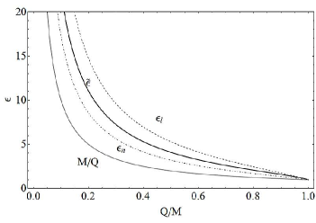
Figure 1: The charge parameters $\epsilon_{l}$ (dashed curve) –defined in Eq.(19)–, ${\widetilde{\epsilon}}$ (black solid curve), $\epsilon_{n}$ (dotdashed curve), and $M/Q$ (gray curve) as functions of the charge–to–mass ratio of the RN black hole.

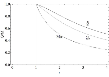
Figure 2: The charge parameters $Q_{n}$ (gray curve), $\widetilde{Q}$ (black solid curve), and $M/\epsilon$ (dashed curve) as functions of the charge–to–mass ratio $\epsilon$ of the test particle.

The behavior of these parameters is depicted in figures 1 and 2.

Moreover, let us introduce the radii

$$r_{\gamma}^{\pm}\equiv\frac{3M}{2}\pm\frac{1}{2}\sqrt{9M^{2}-8Q^{2}},$$ (13)

which represents the limiting radius at which neutral particles (photons) can be in circular motion around a RN black hole Pugliese:2010ps ,

$$r^{\pm}_{l} \equiv \frac{3M}{2}\pm\frac{1}{2}\sqrt{9M^{2}-8Q^{2}-Q^{2}\epsilon^{2}}\ ,$$ (14)

where $\lim_{\epsilon\rightarrow 0}r_{l}^{\pm}=r_{\gamma}^{\pm}$, and

$$r_{s}^{\pm}\equiv\frac{\left(\epsilon^{2}-1\right)Q^{2}M}{\epsilon^{2}Q^{2}-M^{2}}\pm\sqrt{\frac{\epsilon^{2}Q^{4}\left(\epsilon^{2}-1\right)\left(M^{2}-Q^{2}\right)}{\left(\epsilon^{2}Q^{2}-M^{2}\right)^{2}}}\ ,$$ (15)

which corresponds to a zero angular momentum circular orbit (ZAMPs)

$$L=0,\quad\frac{dV}{dr}=0$$ (16)

as seen by an observer at infinity. This special radius generalizes the concept of the classical radius $r_{*}=Q^{2}/M$ which is the limiting value for neutral test particles.

Furthermore, the parameter

$$L^{2}_{n}\equiv\frac{9M^{7}}{2\epsilon^{2}Q^{2}}\left(3M+\sqrt{9M^{2}-8Q^{2}}\right)+\frac{2Q^{2}M^{2}}{\epsilon^{2}}\left(1+\epsilon^{2}\right)$$

$$-\frac{M^{3}}{2\epsilon^{2}}\left[27M+5\sqrt{9M^{2}-8Q^{2}}+3\left(3M+\sqrt{9M^{2}-8Q^{2}}\right)\epsilon^{2}\right],$$ (17)

represents the value of the angular momentum which satisfies the relationship $(dV/dr)(L_{n},r_{\gamma}^{+})=0$.

A careful analysis of the circular orbits properties shows that it is convenient to split the classification problem into two different groups. The first group contains all the negative test charges and positive test charges with $\epsilon\leq 1$. The second group contains only positive test charges with $\epsilon>1$. For both groups we investigate the values of the allowed orbit’s radius and the corresponding angular momentum. The results are summarized for $\epsilon\leq 1$ in Table 1,

Table 1: Characteristics of the circular orbits for charged test particles with charge–to–mass ratio $\epsilon\leq 1$ in a RN black hole.

$\epsilon\in]0,1]$			$\epsilon<0$
Region	Momentum	Region	Momentum
$r=r_{l}^{+}$	$L=\pm L_{-}$	$r>r_{\gamma}^{+}$	$L=\pm L_{+}$
$r_{l}^{+}<r<r_{\gamma}^{+}$	$L=\pm L_{\pm}$
$r=r_{\gamma}^{+}$	$L=\pm L_{n}$
$r>r_{\gamma}^{+}$	$L=\pm L_{-}$

and for $\epsilon>1$ in Tables 3 and 4. Moreover, the characteristic parameters for all the different cases are listed in Table 2.

Table 2: Values of the angular momentum $L$ which are possible in different regions of the radial coordinate $r$.

	Class I		Class II		Class III
	Region	Momentum	Region	Momentum	Region	Momentum
	$r=r_{l}^{+}$	$L=\pm L_{-}$	$r=r_{l}^{+}$	$L=\pm L_{-}$	$r=r_{l}^{+}$	$L=\pm L_{-}$
	$(r_{l}^{+},r_{\gamma}^{+})$	$L=\pm L_{\pm}$	$(r_{l}^{+},r_{\gamma}^{+})$	$L=\pm L_{\pm}$	$(r_{l}^{+},r_{\gamma}^{+})$	$L=\pm L_{\pm}$
	$r=r_{\gamma}^{+}$	$L=\pm L_{n}$	$r=r_{\gamma}^{+}$	$L=\pm L_{n}$	$r=r_{\gamma}^{+}$	$L=0$
	$(r_{\gamma}^{+},\infty)\ \ \ \$	$L=\pm L_{-}$	$(r_{\gamma}^{+},r_{s}^{+})$	$L=\pm L_{-}$
	Class IV		Class V		Class VI
	Region	Momentum	Region	Momentum	Region	Momentum
	$r=r_{l}^{+}$	$L=\pm L_{-}$	$r=r_{l}^{+}(r_{s}^{+})$	$L=0$	$r=r_{l}^{+}$	$L=\pm L_{-}$
	$(r_{l}^{+},r_{s}^{+})$	$L=\pm L_{\pm}$	$(r_{l}^{+},r_{\gamma}^{+})((r_{s}^{+},r_{\gamma}^{+}))\ \ \ \$	$L=\pm L_{+}$	$(r_{l}^{+},r_{\gamma}^{+})$	$L=\pm L_{\pm}$
	$r=r_{s}^{+}$	$L=\pm L_{+};\ L=0$			$r=r_{\gamma}^{+}$	$L=\pm L_{n}$
	$(r_{s}^{+},r_{\gamma}^{+})$	$L=\pm L_{+}$			$(r_{\gamma}^{+},r_{s}^{+})$	$L=\pm L_{-}$
					$r=r_{s}^{+}$	$L=0$
	Class VII		Class VIII		Class IX
	Region	Momentum	Region	Momentum	Region	Momentum
	$r=r_{l}^{+}(r_{s}^{+})$	$\pm L_{-}$	$r=r_{l}^{+}$	$L=0$	$r=r_{s}^{+}$	$L=0$
	$(r_{l}^{+},r_{s}^{+})$	$L=\pm L_{\pm}$	$(r_{l}^{+},r_{\gamma}^{+})\ \ \ \$	$L=\pm L_{+}$	$(r_{s}^{+},r_{\gamma}^{+})$	$L=\pm L_{+}$
	$r=r_{s}^{+}$	$L=0$	$r=r_{\gamma}^{+}$	$L=\pm L_{n}$

Table 3: Classification of the circular orbits of a charged test particle with charge–to–mass ratio $\epsilon>1$ in terms of the value of the ratio $Q/M$ of a RN black hole.

$Q/M\in(0,1/2]\ \$		$Q/M\in[1/2,\sqrt{13}/5)$		$Q/M\in[\sqrt{13}/5,\sqrt{2/3})$		$Q/M\in[\sqrt{2/3},1)$
Region	Class	Region	Class	Region	Class	Region	Class
$\epsilon\in]1,2]$	$\mathbf{I}$	$\epsilon\in]1,M/Q]$	$\mathbf{I}$	$\epsilon\in]1,M/Q]$	$\mathbf{I}$	$\epsilon\in]1,M/Q]$	$\mathbf{I}$
$\epsilon\in]2,M/Q]$	$\mathbf{I}$	$\epsilon\in]M/Q,2]$	$\mathbf{II}$	$\epsilon\in]M/Q,\epsilon_{n}]$	$\mathbf{II}$	$\epsilon\in]M/Q,\epsilon_{n}]$	$\mathbf{II}$
$\epsilon\in]M/Q,\epsilon_{n}]$	VI	$\epsilon\in]2,\epsilon_{n}[$	VI	$\epsilon=\epsilon_{n}$	$\mathbf{III}$	$\epsilon=\epsilon_{n}$	$\mathbf{III}$
$\epsilon=\epsilon_{n}$	$\mathbf{VII}$	$\epsilon=\epsilon_{n}$	$\mathbf{VII}$	$\epsilon\in]\epsilon_{n},2]$	$\mathbf{IV}$	$\epsilon\in]\epsilon_{n},\widetilde{\epsilon}[$	$\mathbf{IV}$
$\epsilon\in]\epsilon_{n},\widetilde{\epsilon}[$	IV	$\epsilon\in]\epsilon_{n},\widetilde{\epsilon}[$	IV	$\epsilon\in]2,\widetilde{\epsilon}[$	$\mathbf{IV}$	$\epsilon\in]\widetilde{\epsilon},2]$	$\mathbf{V}$
$\epsilon=\widetilde{\epsilon}$	VIII	$\epsilon=\widetilde{\epsilon}$	VIII	$\epsilon=\widetilde{\epsilon}$	$\mathbf{VIII}$	$\epsilon>2$	$\mathbf{\mathbf{IX}}$
$\epsilon>\widetilde{\epsilon}$	$\mathbf{IX}$	$\epsilon>\widetilde{\epsilon}$	$\mathbf{IX}$	$\epsilon>\widetilde{\epsilon}$	$\mathbf{IX}$

Table 4: Classification in terms of the charge–to–mass ratio $\epsilon>1$ of the circular orbits of a charged test particle moving in the field of a RN black hole with mass $M$ and charge $Q$.

$\epsilon\in]1,2]$		$\epsilon>2$
Region	Class	Region	Class
$Q\in]0,M/\epsilon]$	I	$Q\in]0,M/\epsilon]$	I
$Q\in]M/\epsilon,Q_{n}[$	$\mathbf{II}$	$Q\in]M/\epsilon,Q_{n}[$	VI
$Q=Q_{n}$	III	$Q=Q_{n}$	VII
$Q\in]Q_{n},\widetilde{Q}[$	IV	$Q\in]Q_{n},\widetilde{Q}[$	IV
$Q\in[\widetilde{Q},M[$	V	$Q=\widetilde{Q}$	VIII
		$Q\in]\widetilde{Q},M[$	IX

We can summarize the results as follows. For $\epsilon\leq 1$ , Table 1, the infimum circular orbital radius is located at $r_{\gamma}^{+}$ ($r_{l}^{+}$) for $\epsilon<0$ ($0<\epsilon\leq 1$). For negative values of $\epsilon$, circular motion can occur for any radius greater than the infimum value $r_{\gamma}^{+}$. The situation is much more complicated for positive values of $\epsilon$ within the interval $0<\epsilon\leq 1$. In this case, the electromagnetic interaction is repulsive, but it is balanced by the attractive gravitational component. The region in which circular orbits are allowed is split by the radius $r_{\gamma}^{+}$ and $r_{l}^{+}$, and in each sub-region different values of the angular momentum from the set $\{\pm L_{\pm},\pm L_{n}\}$ are possible.

The case $\epsilon>1$ should be considered apart. This corresponds to the real case of charged elementary particles, like electrons, protons and ions, orbiting around a charged source and hence several possibilities for realistic motion exist. In the case $\epsilon Q>0$, with $\epsilon>1$, the circular motion dynamics is determined by the classification given in Table 3, for a fixed source charge-to-mass ratio, or in Table 4, for a fixed particle charge-to-mass ratio.

First, we can recognize nine different situations listed in Table 2. There are orbits with angular momentum $L=\pm L_{\pm}$, $L=\pm L_{n}$ or even $L=0$. As mentioned above, this last case occurs when the particle is located at rest with respect to an observer at infinity. Clearly, these particular “orbits” are the consequence of the full balance between the attraction and repulsion among test particles and sources. The infimum circular orbital radius can be $r=r_{\gamma}^{+}$, $r=r_{l}^{+}$ or also $r=r_{s}^{+}$. Comparing with the case $\epsilon<1$, we can clearly see that the main difference between the two cases consists in the presence of a supremum circular orbital radius at $r=r_{\gamma}^{+}$ or at $r=r_{s}^{+}$. This means that the repulsive electromagnetic effect, predominant at larger distances, does not allow circular orbits around the source. The classifications of Table 3 and Table 4 are alternative and equivalent. In the first one, if we fix the charge-to-mass ratio of the black hole, and we move towards increasing values of the particle charge-to-mass ratio, we propose to divide all the possible scenarios into four classes of objects characterized by

$${\mathbf{I}}:Q/M\in(0,1/2],\quad{\mathbf{II}}:Q/M\in(1/2,\sqrt{13}/5]\ ,$$ (18)

$${\mathbf{III}}:Q/M\in(\sqrt{13}/5,\sqrt{2/3})\;{\textbf{IV}}:Q/M\in]\sqrt{2/3},1),$$

respectively. Thus, for a fixed charge of the spacetime, and following Table 3 and Table 2, we can trace a picture of the dynamical properties of that spacetime. An example is provided in figure 3 and figure 4, where the case of a spacetime of charge-to-mass ratio $Q/M=0.1$ is illustrated.

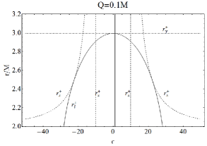
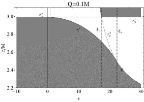
Figure 3: Black hole case with $Q=0.1M$. Left panel: The radii $r_{s}^{+}$, $r_{l}^{+}$ and $r_{\gamma}^{+}$ are plotted as functions of the test particle charge-to-mass ratio $\epsilon$. Shaded regions are forbidden (right panel).

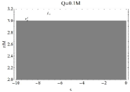
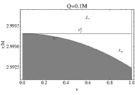
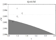
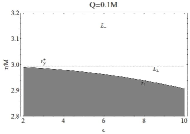
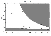
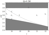
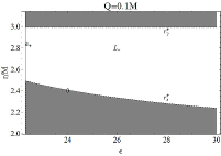
Figure 4: Black hole case with $Q=0.1M$. Shaded regions are forbidden. The radii $r_{s}^{+}$, $r_{l}^{+}$ and $r_{\gamma}^{+}$ are plotted as functions of the test particle charge-to-mass ratio $\epsilon$ in the region $[-10,30]$.

On the other hand, in Table 4, if we fix the charge-to-mass ratio of the test particle, and move towards increasing values of the charge-to-mass ratio of the source, we find only two different cases: $\epsilon\leq 2$ and $\epsilon>2$. In conclusion, using this classification, we can determine the orbital radius followed by the selected particle in the fixed spacetime.

4 Circular motion around a RN naked singularity

Equations  (6) govern the circular motion around a RN naked singularity ($Q\geq M$) as well. Because (7) and (9) define the angular momentum $L_{\pm}$ and the energy $E_{\pm}$ in terms of $r/M$, $Q/M$, and $\epsilon$, it is necessary to investigate several intervals of values where circular motion is allowed. To this end, it is useful to introduce the following notation

$$\epsilon_{l} \equiv \frac{\sqrt{9M^{2}-8Q^{2}}}{Q},$$ (19)

$$\widetilde{\epsilon}_{\pm} \equiv \frac{1}{\sqrt{2}Q}\sqrt{5M^{2}\pm 4Q^{2}+\sqrt{25M^{2}-24Q^{2}}}\ ,$$ (20)

$$\widetilde{\widetilde{\epsilon}}_{\pm} \equiv \frac{1}{\sqrt{2}Q}\sqrt{3M^{2}-2Q^{2}\pm M\sqrt{9M^{2}-8Q^{2}}}\ ,$$ (21)

where $\widetilde{\epsilon}_{-}=\widetilde{\epsilon}$ and $\widetilde{\widetilde{\epsilon}}_{+}=\epsilon_{n}$ as defined in Eqs.(10) and (11), respectively. These limiting values for the particle charge must be real and positive, therefore, the ranges of definitions for the charges $(\epsilon_{l},\widetilde{\epsilon}_{\pm},\widetilde{\widetilde{\epsilon}}_{\pm})$ are chosen in accordance with the positive roots of the Eqs. (19,20) and Eq. (21) in terms of the charge-to-mass ratio $Q/M$ of the naked singularity. For completeness, and following PuQueRu-charge , we reproduce here in Fig.  5 the behavior of these parameters in terms of the ratio $Q/M>1$, where the definition domains for the charges $(\epsilon_{l},\widetilde{\epsilon}_{\pm},\widetilde{\widetilde{\epsilon}}_{\pm})$ are also shown.

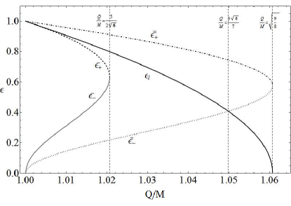
Figure 5: The charge parameters $\epsilon_{l}$, ${\widetilde{\epsilon}}_{\pm}$, and $\widetilde{\widetilde{\epsilon}}_{\pm}$ as functions of the charge–to–mass ratio of the RN naked singularity. The special lines $Q/M=5/\left(2\sqrt{6}\right)\approx 1.02$, $Q/M=3\sqrt{6}/7\approx 1.05$, and $Q/M=\sqrt{9/8}\approx 1.06$ are also plotted.

The special points where ${\widetilde{\epsilon}}_{+}={\widetilde{\epsilon}}_{-}$, $\epsilon_{l}=\widetilde{\widetilde{\epsilon}}_{-}$ and $\widetilde{\widetilde{\epsilon}}_{+}=\widetilde{\widetilde{\epsilon}}_{-}$ correspond to three special values of the ratio $Q/M$ that define four different intervals as follows:

$${\mathbf{I}}:Q/M\in(1,5/(2\sqrt{6})],\;$$ (22)

$${\mathbf{II}}:Q/M\in(5/(2\sqrt{6}),(3\sqrt{6})/7]\ ,\;$$

$${\mathbf{III}}:Q/M\in((3\sqrt{6})/7,\sqrt{9/8}]\ ,\;$$

$${\mathbf{IV}}:Q/M\in[\sqrt{9/8},\infty).$$

Furthermore, it turns out that the properties of circular orbits drastically depends on the sign of the test charge. Moreover, particles with charges within the interval $-1<\epsilon<1$ present a very rich structure of possible circular orbits. We therefore analyze separately positive and negative test charges in two different intervals.

4.1 Positive test charges

For $\epsilon>0$, in general, circular orbits exist in the region $r>r_{*}\equiv Q^{2}/M$. This means that, in the repulsive case, even a small electric charge generates a drastic change in the structure of circular orbits in a NS spacetime, making this an extremely sensitive case. We therefore introduce a classification of naked singularities which includes four classes ($\mathbf{I_{<}^{+}}$, $\mathbf{II_{<}^{+}}$, $\mathbf{III_{<}^{+}}$, $\mathbf{V_{<}^{+}}$) in the interval of small charges, $0<\epsilon<1$, and two classes ($\mathbf{I>^{+}}$, $\mathbf{II>^{+}}$) for large charges, $\epsilon>1$.

In the case of small test charges, it is necessary to consider separately all the possible values of the charge parameters $\epsilon_{l}$, $\widetilde{\epsilon}_{\pm}$ and $\widetilde{\widetilde{\epsilon}}_{\pm}$ in all the regions determined by the four classes of naked singularities given in (22). The angular momentum of the test particles depends on the value of the charge-to-mass ration $\epsilon$ and the distance $r$ from the origin of coordinates. The results are schematically represented in the Tables (5)–(8). A detailed analysis of the behavior of the energy and angular momentum of positive test charges is presented in the figures of given in A.

Table 5: Class $\mathbf{I_{<}^{+}}$: $M<Q\leq 5/(2\sqrt{6})M$ for a test particle charge-to-mass ratio $\epsilon\in]0,1[$.

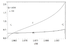
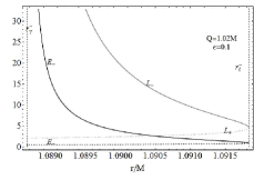
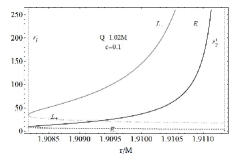
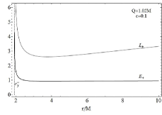
Figure 6: Class: $M<Q\leq 5/(2\sqrt{6})M$ and $0<\epsilon\leq\widetilde{\widetilde{\epsilon}}_{-}$. Parameter choice: $Q=1.02M$ and $\epsilon=0.1$. Then $\widetilde{\widetilde{\epsilon}}_{-}=0.215376$, $r_{s}^{+}=1.06185M$, $r_{\gamma}^{-}=1.08866M$, $r_{\gamma}^{+}=1.91134M$, $r_{l}^{-}=1.09183M$, and $r_{l}^{+}=1.90817M$. Circular orbits exist with angular momentum $L=L^{-}$ (gray curve) and energy $E=E^{-}$ (black curve) in $r_{s}^{+}<r<r_{\gamma}^{-}$; $L=0$ at $r=r_{s}^{+}$ (upper left plot); $L=L_{\pm}$ in $r_{\gamma}^{-}<r\leq r_{l}^{-}$ (upper right plot) and in $r_{l}^{+}\leq r<r_{\gamma}^{+}$ (bottom left plot); $L=L^{-}$ in $r\geq r_{\gamma}^{+}$ (bottom right plot). The angular momentum $L_{+}$ is represented by a gray dotted curve and the energy $E_{+}$ by a black dashed curve.

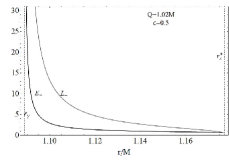
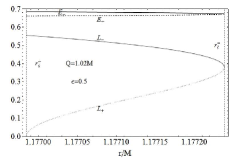
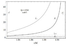
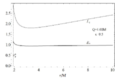
Figure 7: Class: $M<Q\leq 5/(2\sqrt{6})M$ and $\widetilde{\widetilde{\epsilon}}_{-}<\epsilon<\widetilde{\epsilon}_{-}$. Parameter choice: $Q=1.02M$ and $\epsilon=0.5$. Then $\widetilde{\widetilde{\epsilon}}_{-}=0.215376$, $\widetilde{\epsilon}_{-}=0.564915$, $r_{s}^{+}=1.17698M$, $r_{\gamma}^{-}=1.08866M$, $r_{\gamma}^{+}=1.91134M$, $r_{l}^{-}=1.17724M$, and $r_{l}^{+}=1.82276M$. Circular orbits exist with angular momentum $L=L_{+}$ (gray curve) and energy $E=E_{+}$ (black curve) in $r_{\gamma}^{-}<r<r_{s}^{+}$ (upper left plot); $L=L_{\pm}$ in $r_{s}^{+}\leq r<r_{l}^{-}$ (upper right plot) and $r_{l}^{+}\leq r<r_{\gamma}^{+}$ (bottom left plot); $L=L^{-}$ in $r\geq r_{\gamma}^{+}$ (bottom right plot). The angular momentum $L^{-}$ (gray dotted curve) and the energy $E^{-}$ (black dashed curve) are also plotted.

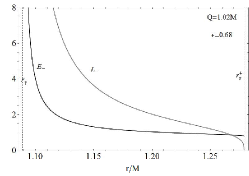
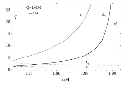
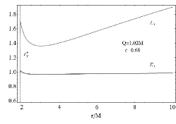
Figure 8: Class: $M<Q\leq 5/(2\sqrt{6})M$ and $\widetilde{\epsilon}_{-}\leq\epsilon\leq\widetilde{\epsilon}_{+}$. Parameter choice: $Q=1.02M$ and $\epsilon=0.68$. Then $\widetilde{\epsilon}_{-}=0.564915$, $\widetilde{\epsilon}_{+}=0.697649$ $r_{s}^{+}=1.27878M$, $r_{\gamma}^{-}=1.08866M$, $r_{\gamma}^{+}=1.91134M$, $r_{l}^{-}=1.2788M$ and $r_{l}^{+}=1.7212M$. Circular orbits exist with angular momentum $L=L_{+}$ (gray curve) and energy $E=E_{+}$ (black curve) in $r_{\gamma}^{-}<r<r_{s}^{+}$ (left plot); $L=0$ at $r=r_{s}^{+}$; $L=L_{\pm}$ in $r_{l}^{+}\leq r<r_{\gamma}^{+}$ (center plot); $L=L^{-}$ in $r\geq r_{\gamma}^{+}$ (right plot).

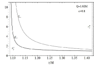
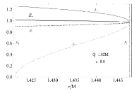
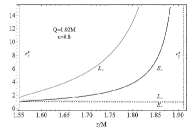
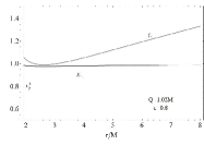
Figure 9: Class: $M<Q\leq 5/(2\sqrt{6})M$ and $\widetilde{\epsilon}_{+}<\epsilon\leq\epsilon_{l}$. Parameter choice: $Q=1.02M$ and $\epsilon=0.8$. Then $\epsilon_{l}=0.806548$, $\widetilde{\epsilon}_{+}=0.697649$, $r_{s}^{+}=1.42131M$, $r_{\gamma}^{-}=1.08866M$, $r_{\gamma}^{+}=1.91134M$, $r_{l}^{-}=1.44769M$, and $r_{l}^{+}=1.55231M$. Circular orbits exist with angular momentum $L=L_{+}$ (gray curves) and energy $E=E_{+}$ (black curves) in $r_{\gamma}^{-}<r<r_{s}^{+}$ (upper left plot); $L=L_{\pm}$ in $r_{s}^{+}\leq r<r_{l}^{-}$ (upper right plot) and $r_{l}^{+}\leq r<r_{\gamma}^{+}$ (bottom left plot); $L=L^{-}$ in $r\geq r_{\gamma}^{+}$ (bottom right plot).

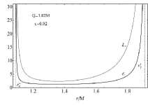
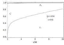
Figure 11: Class: $M<Q\leq 5/(2\sqrt{6})M$ and $\widetilde{\widetilde{\epsilon}}_{+}\leq\epsilon<M/Q$. Parameter choice: $Q=1.02M$ and $\epsilon=0.92$. Then $\widetilde{\widetilde{\epsilon}}_{+}=0.914942$, $M/Q=0.980392,$ $r_{s}^{+}=1.96981M$, $r_{\gamma}^{-}=1.08866M$, and $r_{\gamma}^{+}=1.91134M$. Circular orbits exist with angular momentum $L=L_{+}$ (gray curves) and energy $E=E_{+}$ (black curves) in $r_{\gamma}^{-}<r<r_{\gamma}^{+}$ (left plot) and $L=L^{-}$ in $r>r_{s}^{+}$ (right plot).

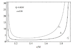
Figure 12: Class: $M<Q\leq 5/(2\sqrt{6})M$ and $M/Q\leq\epsilon<1$. Parameter choice: $Q=1.02M$ and $\epsilon=0.99$. Then $\widetilde{\widetilde{\epsilon}}_{+}=0.914942$, $r_{s}^{+}=0.431596M$, $r_{\gamma}^{-}=1.08866M$, and $r_{\gamma}^{+}=1.91134M$. Circular orbits exist with angular momentum $L=L_{+}$ (gray curve) and energy $E=E_{+}$ (black curve) in $r_{\gamma}^{-}<r<r_{\gamma}^{+}$.

	a): $0<\epsilon\leq\widetilde{\widetilde{\epsilon}}_{-}$ Fig. (6)		b): $\widetilde{\widetilde{\epsilon}}_{-}<\epsilon<\widetilde{\epsilon}_{-}$ Fig. (7)		c): $\widetilde{\epsilon}_{-}\leq\epsilon\leq\widetilde{\epsilon}_{+}$ Fig. (8)
	Region	Momentum	Region	Momentum	Region	Momentum
	$r=r_{s}^{+}$	$L=0$	$(r_{\gamma}^{-},r_{s}^{+})$	$L=\pm L_{+}$	$(r_{\gamma}^{-},r_{s}^{+})$	$L=\pm L_{+}$
	$(r_{s}^{+},r_{\gamma}^{-})$	$L=\pm L_{-}$	$[r_{s}^{+},r_{l}^{-})$	$L=\pm L_{\pm}$	$r=r_{s}^{+}$	$L=0$
	$(r_{\gamma}^{-},r_{l}^{-}]$	$L=\pm L_{\pm}$	$[r_{l}^{+},r_{\gamma}^{+})$	$L=\pm L_{\pm}$	$[r_{l}^{+},r_{\gamma}^{+})$	$L=\pm L_{\pm}$
	$[r_{l}^{+},r_{\gamma}^{+})$	$L=\pm L_{\pm}$	$r\geq r_{\gamma}^{+}$	$L=\pm L_{-}$	$r\geq r_{\gamma}^{+}$	$L=\pm L_{-}$
	$r\geq r_{\gamma}^{+}$	$L=\pm L_{-}$
	d): $\widetilde{\epsilon}_{+}<\epsilon\leq\epsilon_{l}$ Fig. (9)		e): $\epsilon_{l}<\epsilon<\widetilde{\widetilde{\epsilon}}_{+}$ Fig. (8)		f): $\widetilde{\widetilde{\epsilon}}_{+}\leq\epsilon<M/Q$ Fig. (11)
	Region	Momentum	Region	Momentum	Region	Momentum
	$(r_{\gamma}^{-},r_{s}^{+})$	$L=\pm L_{+}$	$(r_{\gamma}^{-},r_{s}^{+})$	$L=\pm L_{+}$	$(r_{\gamma}^{-},r_{\gamma}^{+})$	$L=\pm L_{+}$
	$[r_{s}^{+},r_{l}^{-})$	$L=\pm L_{\pm}$	$[r_{s}^{+},r_{\gamma}^{+})$	$L=\pm L_{\pm}$	$r>r_{s}^{+}$	$L=\pm L_{-}$
	$[r_{l}^{+},r_{\gamma}^{+})$	$L=\pm L_{\pm}$	$r\geq r_{\gamma}^{+}$	$L=\pm L_{-}$
	$r\geq r_{\gamma}^{+}$	$L=\pm L_{-}$
	g) $M/Q\leq\epsilon<1$ Fig. (12)
	Region	Momentum
	$(r_{\gamma}^{-},r_{\gamma}^{+})$	$\pm L_{+}$

Table 6: Class $\mathbf{II_{<}^{+}}$: $5/(2\sqrt{6})M<Q<(3\sqrt{6}/7)M$, for a test particle charge-to-mass ratio $\epsilon\in]0,1[$.

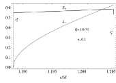
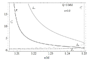
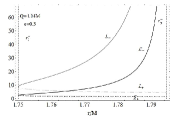
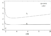
Figure 13: Class: $5/(2\sqrt{6})M<Q<(3\sqrt{6}/7)M$ and $0<\epsilon<\widetilde{\widetilde{\epsilon}}_{-}$. Parameter choice: $Q=1.04M$ and $\epsilon=0.3$. Then $\widetilde{\widetilde{\epsilon}}_{-}=0.338294$, $r_{s}^{+}=1.18836M$, $r_{\gamma}^{-}=1.20538M$, $r_{\gamma}^{+}=1.79462M$, $r_{l}^{-}=1.25007M$, and $r_{l}^{+}=1.74993M$. Circular orbits exist with angular momentum $L=L^{-}$ (gray curves) and energy $E=E^{-}$ (black curves) in $r_{s}^{+}<r\leq r_{\gamma}^{-}$ (upper left plot); $L=0$ at $r=r_{s}^{+}$; $L=L_{\pm}$ in $r_{\gamma}^{-}<r\leq r_{l}^{-}$ (upper right plot) and $r_{l}^{+}\leq r<r_{\gamma}^{+}$ (bottom left plot); $L=L^{-}$ in $r\geq r_{\gamma}^{+}$ (bottom right plot).

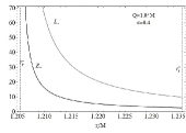
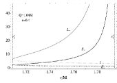
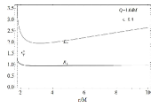
Figure 14: Class: $5/(2\sqrt{6})M<Q<(3\sqrt{6}/7)M$ and $\widetilde{\widetilde{\epsilon}}_{-}<\epsilon<\epsilon_{l}$. Parameter choice: $Q=1.04M$ and $\epsilon=0.4$. Then $\widetilde{\widetilde{\epsilon}}_{-}=0.338294$, $\epsilon_{l}=0.566574$, $r_{s}^{+}=1.23565M$, $r_{\gamma}^{-}=1.20538M$, $r_{\gamma}^{+}=1.79462M$, $r_{l}^{-}=1.29135M$, and $r_{l}^{+}=1.70865M$. Circular orbits exist with angular momentum $L=L_{+}$ (gray curve) and energy $E=E_{+}$ (black curve) in $r_{\gamma}^{-}<r<r_{s}^{+}$ (upper left plot); $L=0$ at $r=r_{s}^{+}$; $L=L_{\pm}$ in $r_{s}^{+}<r<r_{l}^{-}$ (upper right plot) and $r_{l}^{+}\leq r<r_{\gamma}^{+}$ (bottom left plot); $L=L^{-}$ in $r\geq r_{\gamma}^{+}$ (bottom right plot).

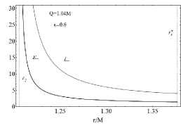
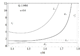
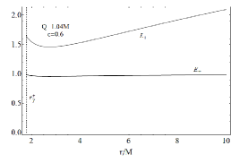
Figure 15: Class: $5/(2\sqrt{6})M<Q<(3\sqrt{6}/7)M$ and $\epsilon_{l}\leq\epsilon\leq\widetilde{\widetilde{\epsilon}}_{+}$. Parameter choice: $Q=1.04M$ and $\epsilon=0.6$. Then $\widetilde{\widetilde{\epsilon}}_{+}=0.811927$ and $\epsilon_{l}=0.566574$, $r_{s}^{+}=1.37651M$, $r_{\gamma}^{-}=1.20538M$, and $r_{\gamma}^{+}=1.79462M$. Circular orbits exist with angular momentum $L=L_{+}$ (gray curve) and energy $E=E_{+}$ (black curve) in $r_{\gamma}^{-}<r<r_{s}^{+}$ (left plot); $l=L_{\pm}$ in $r_{s}^{+}\leq r<r_{\gamma}^{+}$ (center plot); and $L=L^{-}$ in $r\geq r_{\gamma}^{+}$ (right plot).

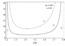
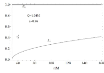
Figure 16: Class: $5/(2\sqrt{6})M<Q<(3\sqrt{6}/7)M$ and $\widetilde{\widetilde{\epsilon}}_{+}\leq\epsilon<M/Q$. Parameter choice: $Q=1.04M$ and $\epsilon=0.96$. Then $\widetilde{\widetilde{\epsilon}}_{+}=0.811927$, $M/Q=0.961538$ $r_{s}^{+}=52.4944M$, $r_{\gamma}^{-}=1.20538M$, and $r_{\gamma}^{+}=1.79462M$. Circular orbits exist with angular momentum $L=L_{+}$ (gray curve) and energy $E=E_{+}$ (black curve) in $r_{\gamma}^{-}<r<r_{\gamma}^{+}$ ( left plot) and $L=L^{-}$ in $r>r_{s}^{+}$; $L=0$ at $r=r_{s}^{+}$ (right plot).

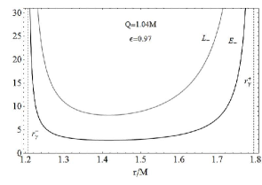
Figure 17: Class: $5/(2\sqrt{6})M<Q<(3\sqrt{6}/7)M$ and $M/Q\leq\epsilon<1$. Parameter choice: $Q=1.04M$ and $\epsilon=0.97$, Then $\widetilde{\widetilde{\epsilon}}_{+}=0.866828$, $M/Q=0.961538$, $r_{\gamma}^{-}=1.20538M$, and $r_{\gamma}^{+}=1.79462M$. Circular orbits exist with $L=L_{+}$ (gray curve) and $E=E_{+}$ (black curve) in $r_{\gamma}^{-}<r<r_{\gamma}^{+}$.

	a): $0<\epsilon<\widetilde{\widetilde{\epsilon}}_{-}$ Fig. (13)		b): $\widetilde{\widetilde{\epsilon}}_{-}<\epsilon<\epsilon_{l}$ Fig. (14)		c): $\epsilon_{l}\leq\epsilon\leq\widetilde{\widetilde{\epsilon}}_{+}$ Fig. (15.)
	Region	Momentum	Region	Momentum	Region	Momentum
	$r=r_{s}^{+}$	$L=0$	$(r_{\gamma}^{+},r_{s}^{+})$	$L=\pm L_{+}$	$(r_{\gamma}^{+},r_{s}^{+})$	$L=\pm L_{+}$
	$(r_{s}^{+},r_{\gamma}^{-}]$	$L=\pm L_{-}$	$r=r_{s}^{+}$	$L=0$	$[r_{s}^{+},r_{\gamma}^{+})$	$L=\pm L_{\pm}$
	$(r_{\gamma}^{-},r_{l}^{-}]$	$L=\pm L_{\pm}$	$(r_{s}^{+},r_{l}^{-})$	$L=\pm L_{\pm}$	$r\geq r_{\gamma}^{+}$	$L=\pm L_{-}$
	$[r_{l}^{+},r_{\gamma}^{+})$	$L=\pm L_{\pm}$	$[r_{l}^{+},r_{\gamma}^{+})$	$L=\pm L_{\pm}$
	$r\geq r_{\gamma}^{+}$	$L=\pm L_{-}$	$r\geq r_{\gamma}^{+}$	$L=\pm L_{-}$
	d): $\widetilde{\widetilde{\epsilon}}_{+}\leq\epsilon<M/Q$ Fig. (16)		e): $M/Q\leq\epsilon<1$ Fig. (17)
	Region	Momentum	Region	Momentum	Region	Momentum
	$(r_{\gamma}^{-},r_{\gamma}^{+})$	$L=\pm L_{+}$	$(r_{\gamma}^{-},r_{\gamma}^{+})$	$L=\pm L_{+}$
	$r>r_{s}^{+}$	$L=\pm L_{-}$
	$r=r_{s}^{+}$	$L=0$

Table 7: Class $\mathbf{III_{<}^{+}}$: $(3\sqrt{6}/7)M\leq Q\leq\sqrt{9/8}M$, for a test particle charge-to-mass ratio $\epsilon\in]0,1[$.

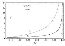
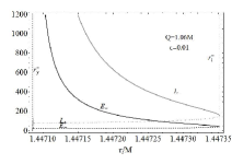
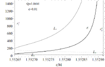
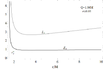
Figure 18: Class: $(3\sqrt{6}/7)M\leq Q\leq\sqrt{9/8}M$ and $0<\epsilon\leq\epsilon_{l}$ Parameter choice: $Q=1.06M$ and $\epsilon=0.01$. Then $\epsilon_{l}=0.0998397$, $r_{s}^{+}=1.12756M$, $r_{\gamma}^{-}=1.44708M$, $r_{\gamma}^{+}=1.55292M$ $r_{l}^{-}=1.44735M$, and $r_{l}^{+}=1.55265M$. Circular orbits exist with angular momentum $L=L^{-}$ (gray curve) and energy $E=E^{-}$ (black curve) in $r_{\gamma}^{-}\leq r\leq r_{l}^{-}$; $L=0$ at $r=r_{s}^{+}$ (upper left plot); $L=L_{\pm}$ in $r_{s}^{+}<r<r_{l}^{-}$ (upper right plot) and $r_{l}^{+}\leq r<r_{\gamma}^{+}$ (bottom left plot); $L=L^{-}$ in $r\geq r_{\gamma}^{+}$ (bottom right plot).

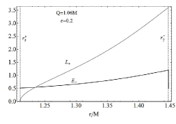
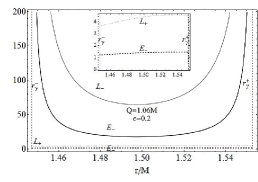
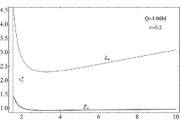
Figure 19: Class: $(3\sqrt{6}/7)M\leq Q\leq\sqrt{9/8}M$ and $\epsilon_{l}<\epsilon\leq\widetilde{\widetilde{\epsilon}}_{-}$. Parameter choice: $Q=1.06M$ and $\epsilon=0.2$. Then $\epsilon_{l}=0.0998397$, $\widetilde{\widetilde{\epsilon}}_{-}=0.536564$, $r_{s}^{+}=1.21047M$, $r_{\gamma}^{-}=1.44708M$, and $r_{\gamma}^{+}=1.55292M$. Circular orbits exist with angular momentum $L=L^{-}$ (gray curve) and energy $E=E^{-}$ (black curve) in $r_{s}^{+}<r<r_{\gamma}^{-}$; $L=0$ at $r=r_{s}^{+}$ (left plot); $L=L_{\pm}$ in $r_{\gamma}^{-}\leq r<r_{\gamma}^{+}$ (center plot); and $L=L^{-}$ in $r\geq r_{\gamma}^{+}$ (right plot).

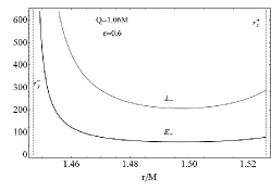
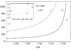
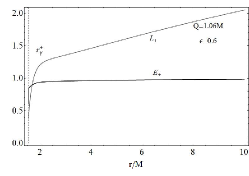
Figure 20: Class: $(3\sqrt{6}/7)M\leq Q\leq\sqrt{9/8}M$ and $\widetilde{\widetilde{\epsilon}}_{-}<\epsilon<\widetilde{\widetilde{\epsilon}}_{+}$. Parameter choice: $Q=1.06M$ and $\epsilon=0.6$. Then $\widetilde{\widetilde{\epsilon}}_{+}=0.618133$, $\widetilde{\widetilde{\epsilon}}_{-}=0.536564$, $r_{s}^{+}=1.52596M$, $r_{\gamma}^{-}=1.44708M$, and $r_{\gamma}^{+}=1.55292M$. Circular orbits exist with angular momentum $L=L_{+}$ (gray curve) and energy $E=E_{+}$ (black curve) in $r_{\gamma}^{-}<r<r_{s}^{+}$ (left plot); $L=L_{\pm}$ in $r_{s}^{+}\leq r<r_{\gamma}^{+}$ (center plot); and $L=L^{-}$ in $r\geq r_{\gamma}^{+}$ (right plot).

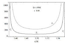
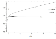
Figure 21: Class: $(3\sqrt{6}/7)M\leq Q\leq\sqrt{9/8}M$ and $\widetilde{\widetilde{\epsilon}}_{+}\leq\epsilon<M/Q$. choice: $Q=1.06M$ and $\epsilon=0.66$. Then $\widetilde{\widetilde{\epsilon}}_{+}=0.618133$, $M/Q=0.943396$ $r_{s}^{+}=1.62572M$, $r_{\gamma}^{-}=1.44708,M$, and $r_{\gamma}^{+}=1.55292M$. Circular orbits exist with angular momentum $L=L_{+}$ (gray curve) and energy $E=E_{+}$ (black curve) in $r_{\gamma}^{-}<r<r_{\gamma}^{+}$ (left plot) and $L=L^{-}$ in $r>r_{s}^{+}$; $L=0$ at $r=r_{s}^{+}$ (right plot).

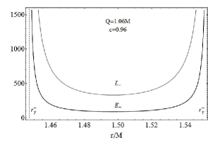
Figure 22: Class: $(3\sqrt{6}/7)M\leq Q\leq\sqrt{9/8}M$ and $M/Q\leq\epsilon<1$. Parameter choice: $Q=1.06M$ and $\epsilon=0.96$. Then $M/Q=0.943396$, $r_{\gamma}^{-}=1.44708,M$ and $r_{\gamma}^{+}=1.55292M$. Circular orbits exist with angular momentum $L=L_{+}$ (gray curve) and energy $E=E_{+}$ (black curve) in $r_{\gamma}^{-}<r<r_{\gamma}^{+}$.

	a): $0<\epsilon\leq\epsilon_{l}$ Fig. (18)		b): $\epsilon_{l}<\epsilon\leq\widetilde{\widetilde{\epsilon}}_{-}$ Fig. (19)		c): $\widetilde{\widetilde{\epsilon}}_{-}<\epsilon<\widetilde{\widetilde{\epsilon}}_{+}$ Fig. (20)
	Region	Momentum	Region	Momentum	Region	Momentum
	$[r_{\gamma}^{-},r_{l}^{-}]$	$L=\pm L_{-}$	$r=r_{s}^{+}$	$L=0$	$(r_{\gamma}^{-},r_{s}^{+})$	$L=\pm L_{+}$
	$r=r_{s}^{+}$	$L=0$	$(r_{s}^{+},r_{\gamma}^{-})$	$L=\pm L_{-}$	$[r_{s}^{+},r_{\gamma}^{+})$	$L=\pm L_{\pm}$
	$(r_{s}^{+},r_{l}^{-})$	$L=\pm L_{\pm}$	$[r_{\gamma}^{-},r_{\gamma}^{+})$	$L=\pm L_{\pm}$	$r\geq r_{\gamma}^{+}$	$L=\pm L_{-}$
	$[r_{l}^{+},r_{\gamma}^{+})$	$L=\pm L_{\pm}$	$r\geq r_{\gamma}^{+}$	$L=\pm L_{-}$
	$r\geq r_{\gamma}^{+}$	$L=\pm L_{-}$
	d): $\widetilde{\widetilde{\epsilon}}_{+}\leq\epsilon<M/Q$ Fig. (21)		e): $M/Q\leq\epsilon<1$ Fig. (22)
	Region	Momentum	Region	Momentum	Region	Momentum
	$(r_{\gamma}^{-},r_{\gamma}^{+})$	$L=\pm L_{+}$	$(r_{\gamma}^{-},r_{\gamma}^{+})$	$L=\pm L_{+}$
	$r=r_{s}^{+}$	$L=0$
	$r>r_{s}^{+}$	$L=\pm L_{+};\ L=\pm L_{-}$
	Class $\mathbf{IV_{<}^{+}}$ $Q>\sqrt{9/8}M$
	$0<\epsilon<M/Q$
	Region	Momentum
	$r=r_{s}^{+}$	$L=0$
	$r>r_{s}^{+}$	$L=\pm L_{-}$

Table 8: Classes for large test charges ($\epsilon>1$).

	Class $\mathbf{I_{>}^{+}}$: $M<Q<\sqrt{9/8}M$			Class $\mathbf{II_{>}^{+}}$: $\sqrt{9/8}M<Q$
	Region	Momentum		Region	Momentum
	$(r^{-}_{\gamma},r^{+}_{\gamma})$	$L=L_{+}$		Forbidden

We see that in the interval of small test charges several subclasses appear which are delimited by the value of the charge parameters $\epsilon_{l}$, $\widetilde{\epsilon}_{\pm}$ and $\widetilde{\widetilde{\epsilon}}_{\pm}$. In general we can summarize the situation as follows. There is always a minimum radius $r_{min}$ at which circular motion is allowed. At the radius $r_{\gamma}^{-}$ the energy of the test particle diverges, indicating that the hypersurface $r=r_{\gamma}^{-}$ is lightlike. In the simplest case, there is a minimum radius $r_{min}$ so that circular orbits are allowed in the infinite interval $]r_{min},\infty)$. Otherwise, this region is split by a lightlike hypersurface situated at $r_{\gamma}^{+}>r_{min}$.

Another possible structure is that of a spatial configuration formed by two separated regions in which circular motion is allowed in a finite region filled with charged particles within the spatial interval $(r_{min}=r_{\gamma}^{-},r_{max}=r_{\gamma}^{+})$. This region is usually surrounded by an empty finite region in which no motion is allowed. Outside the empty region, we find a zone of allowed circular motion in which either only neutral particles or neutral and charged particles can exist in circular motion.

The situation in the case of large charges $(\epsilon>1)$ is simpler. There is only one region in class $\mathbf{I_{>}^{+}}$ in which circular motion can exist. Naked singularities within the Class $\mathbf{II_{>}^{+}}$ do not allow any circular orbits. In fact, since for $\epsilon Q>0$ the Coulomb interaction is repulsive, the configuration characterized by the values $Q\geq\sqrt{9/8}M$ and $\epsilon>1$ corresponds to a repulsive electromagnetic effect that cannot be balanced by an attractive gravitational interaction.

The energy and angular momentum of circular orbits diverge as $r$ approaches the limiting orbits at $r_{\gamma}^{\pm}$; the boundary $r=r_{\gamma}^{+}$ in this case corresponds to a lightlike hypersurface. Finally, the energy of the states is always positive.

4.2 Negative test charges

In the case of test particles with negative charge, the dependence of circular orbits on the charge-to-mass ratio of the naked singularity is simpler than in the case of positive charges. Indeed, we need to consider only two intervals defined as follows:

$$\mathbf{I^{-}}:\ M<Q<\sqrt{9/8}M\quad\mathbf{II^{-}}:\ Q/M>\sqrt{9/8}.$$ (23)

Large negative particle charge-to-mass ratio: For $\epsilon<-1$, the contribution of the electromagnetic interaction is always attractive. Hence, the repulsive force necessary to balance the attractive effects of the Coulomb interactions can be generated only by a RN naked singularity. In particular, for $\epsilon<-1$ and for $Q>\sqrt{9/8}M$ (Class $\mathbf{II^{-}}$) circular orbits with $L=L_{+}$ always exist for $r>0$. For $M<Q\leq\sqrt{9/8}M$ (Class $\mathbf{I^{-}}$), circular orbits exist with $L=L_{+}$ in $0<r<r_{\gamma}^{-}$ and $r>r_{\gamma}^{+}$. Charged test particles with $\epsilon<-1$ can move along circular orbits also in the region $(0,r_{*}]$. The value of the energy on circular orbits increases as $r$ approaches $r=0$, and the angular momentum, as seen by an observer located at infinity, decreases as the radius of the orbit decreases. In the region $M<Q\leq\sqrt{9/8}M$, two limiting orbits appear at $r_{\gamma}^{\pm}$ (similar to the neutral particle case Pugliese:2010ps ).

Small negative particle charge-to-mass ratio: In the case of small charges $(-1<\epsilon<0)$, it is necessary to split the analysis into three different intervals. The results are summarized in Tables 9 and 10. We classify naked singularities into two classes, according to the interval of $Q/M$ to which they belong. In general, two different configurations are allowed. For $Q>\sqrt{9/8}M$ (Class $\mathbf{II^{-}}$) a continuous region appears from a minimum radius $r_{min}\in\{r_{s}^{\pm},Q^{2}/(2M)\}$ to infinity in which circular orbits are allowed. For $M<Q\leq\sqrt{9/8}M$ (Class $\mathbf{I^{-}}$) there is a non connected region $(r_{min},\infty)$ inside which there is a forbidden region $(r_{\gamma}^{-},r_{\gamma}^{+})$. The configuration is therefore composed of two disconnected regions.

In B, we include several figures that depict the behavior of the angular momentum and energy of negative test charges.

Table 9: Class $\mathbf{I^{-}}$ $M<Q\leq\sqrt{9/8}M$

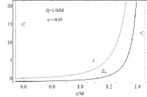
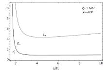
Figure 24: Class: $M<Q\leq\sqrt{9/8}M$ and $-1<\epsilon<-M/Q$. Parameter choice: $Q=1.06M$ and $\epsilon=-0.95$. Then $r_{s}^{+}=0.542901M$, $r_{\gamma}^{-}=1.44708M$, and $r_{\gamma}^{+}=1.55292M$. Circular orbits exist with angular momentum $L=L_{+}$ (gray curve) and energy $E=E_{+}$ (black curve) in $r_{s}^{+}<r<r_{\gamma}^{-}$ (left plot) and in $r>r_{\gamma}^{+}$ for (right plot). For $r=r_{s}^{+}$, $L=0$.

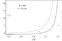
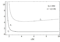
Figure 25: Class: $M<Q\leq\sqrt{9/8}M$ and $\epsilon=-M/Q$. Parameter choice: $Q=1.06M$. Then $Q^{2}/(2M)=0.5618M$, $r_{\gamma}^{-}=1.44708M$ and $r_{\gamma}^{+}=1.55292M$. Circular orbits exist with angular momentum $L=L_{+}$ (gray curve) and energy $E=E_{+}$ (black curve) in $Q^{2}/(2M)<r<r_{\gamma}^{-}$ (left plot) and in $r>r_{\gamma}^{+}$(right plot). For $r=Q^{2}/(2M)$, $L=0$.

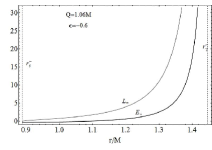
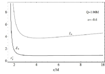
Figure 26: Class: $M<Q\leq\sqrt{9/8}M$ and $-M/Q<\epsilon<0$. Parameter choice: $Q=1.06M$ and $\epsilon=-0.6$. Then $M/Q=0.943396$, $r_{\gamma}^{-}=1.44708M$, $r_{\gamma}^{+}=1.55292M$, and $r_{s}^{-}=0.889152M$. Circular orbits exist with angular momentum $L=L_{+}$ (gray curve) and energy $E=E_{+}$ (black curve) in $r_{s}^{-}<r<r_{\gamma}^{-}$ (left plot) and in $r>r_{\gamma}^{+}$ (right plot). For $r=r_{s}^{-}$, $L=0$.

	a): $\epsilon<-1$		b): $-1<\epsilon<-M/Q$ Fig. (24)		c): $\epsilon=-M/Q$ Fig. (25)
	Region	Momentum	Region	Momentum	Region	Momentum
	$(0,r_{\gamma}^{-})$	$L=\pm L_{+}$	$r=r_{s}^{+}$	$L=0$	$r=Q^{2}/2M$	$L=0$
	$r>r_{\gamma}^{+}$	$L=\pm L_{+}$	$(r_{s}^{+},r_{\gamma}^{-})$	$L=\pm L_{+}$	$(Q^{2}/2M,r_{\gamma}^{-})$	$L=\pm L_{+}$
			$r>r_{\gamma}^{+}$	$L=\pm L_{+}$	$r>r_{\gamma}^{+}$	$L=\pm L_{+}$
	d): $-M/Q<\epsilon<0$ Fig. (26)
	Region	Momentum
	$r=r_{s}^{-}$	$L=0$
	$(r_{s}^{-},r_{\gamma}^{-})$	$L=\pm L_{+}$
	$r>r_{\gamma}^{+}$	$L=\pm L_{+}$

Table 10: Class $\mathbf{II^{-}}$ $Q>\sqrt{9/8}M$

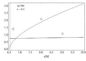
Figure 27: Class: $Q>\sqrt{9/8}M$ and $-1<\epsilon<-M/Q$. Parameter choice: $Q=5M$ and $\epsilon=-0.5$. Then $M/Q=0.2$, $r_{s}^{+}=6.5301M$. Circular orbits exist with angular momentum $L=L_{+}$ (gray curve) and energy $E=E_{+}$ (black curve) in $r>r_{s}^{+}$. For $r=r_{s}^{+}$, $L=0$.

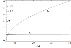
Figure 28: Class: $Q>\sqrt{9/8}M$ and $\epsilon=-M/Q$. Parameter choice: $Q=5M$ and $\epsilon=-0.2$. Then $r_{s}^{+}=16M$. Circular orbits exist with angular momentum $L=L_{+}$ (gray curve) and energy $E=E_{+}$ (black curve) in the region $r>Q^{2}/(2M)$. For $r=Q^{2}/(2M)$, $L=0$.

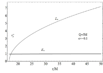
Figure 29: Class: $Q>\sqrt{9/8}M$ and $-M/Q<\epsilon<0$. Parameter choice: $Q=5M$ and $\epsilon=-0.1$. Then $r_{s}^{-}=16.7519M$. Circular orbits exist with angular momentum $L=L_{+}$ (gray curve) and energy $E=E_{+}$ (black curve) in $r>r_{s}^{-}$. For $r=r_{s}^{-}$, $L=0$.

	a): $\epsilon<-1$		b): $-1<\epsilon<-M/Q$ Fig. (27)		c): $\epsilon=-M/Q$ Fig. (28)
	Region	Momentum	Region	Momentum	Region	Momentum
	$r>0$	$L=\pm L_{+}$	$r=r_{s}^{+}$	$L=0$	$r=Q^{2}/2M$	$L=0$
			$r>r_{s}^{+}$	$L=\pm L_{+}$	$r>Q^{2}/2M$	$L=\pm L_{+}$
	d): $-M/Q<\epsilon<0$ Fig. (29)
	Region	Momentum
	$r=r_{s}^{-}$	$L=0$
	$r>r_{s}^{-}$	$L=\pm L_{+}$

5 Discussion and future perspectives

In this work, we explored the motion of charged test particles along circular orbits in the spacetime described by the Reissner–Nordström metric. A detailed discussion of the dynamics for the black hole and naked singularity cases has been performed. Circular orbits have been classified in detail for a complete set of cases.

We adopt the effective potential approach to study test particle orbits in the Reissner–Nordström spacetime, focusing on the equatorial orbits. We explore the morphology of the orbital regions. This analysis leads to a clear differentiation between naked singularities and black holes. A remarkable implication of this description is that the circular orbit configuration in the black hole case is not allowed in the naked singularity regime. Instead, the study of the circular orbits trace out a possible way to distinguish the two physical situations.

In a series of previous works Pugliese:2010ps ; Pugliese:2010he ; PuQueRu-charge , we analyzed the dynamics of the RN spacetime, and studied the motion of neutral and charged test particles, by using the effective potential approach. We showed that in the case of charged test particles the term $\epsilon Q/r$ drastically changes the behavior of the effective potential. The study shows the existence of stability regions whose geometric structure clearly distinguishes naked singularities from black holes (see also Virbhadra:2002ju ; Virbhadra:2007kw and do1 ; Dabrowski:2002iw ). In PuQueRu-charge , in particular, we studied the spatial regions of the RN spacetime where circular motion is allowed around either black holes or naked singularities. We showed that the geometric structure of stable accretion disks allows us to clearly distinguish between black holes and naked singularities. In this work, we presented the complete classification of circular motion around a RN black hole, and around a RN naked singularity with $0<\epsilon<1$ and $-1<\epsilon<0$.

Clearly, this analysis could be used to construct an accretion disk with disconnected rings made of test particles. A precise characterization of matter configurations surrounding a charged compact astrophysical object can account for significant astrophysical processes observed in the electromagnetic band, like the jet emissions. Therefore understanding the dynamics around compact objects is important for the understanding of the accretion disk phenomena and the classification of their general properties.

In the naked singularity case, gravity can assume a repulsive nature that produces a complicated picture of dynamics around the source. We distinguish four regions of charge-to-mass ratio values of the source that characterized these configurations. In each region, different cases can occur: an infinite, continuum, region or otherwise a disconnected region. In the black hole case the circular orbits configuration strongly varies if $\epsilon\leq 1$ or $\epsilon>1$. An infimum radius always appears, and in the case $\epsilon>1$ a supremum circular orbits radius can appear.

The existence of special schemes for circular orbits in RN geometries as outlined in Tables 1,2,3,4,5,6,7,8,9, and 10 show a complicated scenario able to distinguish classes of attractors and particles in motion identified through their charge-to-mass ratios. More importantly, this investigation has enlighten particular limiting values for the BH and NS metric parameters and, remarkably, notable values for the charge-to mass ratio of the orbiting particle. The importance of these studies lies also in the fact that for a long time it has been discussed about the existence and interpretation of the limits of the charge-to-mass ratio and of the dimensionless spin emerging from the General Relativistic formulation of non-quantum self-gravitating objects with electric charge or intrinsic spin. These descriptions have been performed by using the relativistic exact solutions of Kerr, Reissner-Nordström and Kerr-Newman. In the case of black holes, considered in Tables 1,2,3, and 4, the situation is very clear. For negatively charged elementary particles, $\epsilon<0$ (with attractive force $Q\epsilon<0$) the region of circular motion is bounded from below by the photon circular orbit. The situation is definitely complicated for particles with small positive charges, $\epsilon\in]0,1[$, where an articulated structure, determined by the new limiting radius $r_{l}$, appears. The role of the radius $r_{*}=Q^{2}/M$ for zero angular momentum particles (ZAMPs) in BH geometries and $r_{\star}\equiv Q^{2}/2M$ for ZAMPs in NS spacetimes are thoroughly considered, finding a generalization with radius $r_{s}^{+}(Q)$. It is interesting to note that $r_{*}$ corresponds to the value of the classical radius of an electric charge. However this proves that high negative charges (attractive interaction) have some similarities with small charges $\epsilon\in]0,1[$ with repulsive force $(\epsilon Q/M<1)$. The repulsive case however, $Q\epsilon>0$, shows a richer classification of possible cases as $\epsilon$ increases (see Tables 2 and 3). From the rich structure of the cases shown in Table  3, we point out the presence of particular limiting values for black holes, namely $\left.Q/M\right|_{\lim}\in(1/2,\sqrt{13}/5,\sqrt{2/3})$, and for charged particles, namely $\left.\epsilon\right|_{\lim}\in(1,2,M/Q,\epsilon_{n}(Q),\tilde{\epsilon}(Q))$. However, Table 4 clearly shows that $\epsilon=1$ and $\epsilon=2$ are particularly important limiting particle charges. Naked singularities, on the other hand, must be classified as weak $(Q/M<\sqrt{9/8})$ or strong $(Q/M>\sqrt{9/8})$ compact objects. We recognize four classes for the charge parameters with limiting values $\left.Q/M\right|_{\lim}\in(1,5/(2\sqrt{6}),3\sqrt{6}/7,\sqrt{9/8})$, and different values for the particle charge, for instance, $\epsilon_{\lim}=M/Q$. These results are important in the characterization of interactions between self-gravitating charged objects and charged particles, particularly for parameters close to the limiting values pointed out here. Further limits have been studied, for example, in Zakharov:2014lqa . In Blaschke:2016uyo , some limiting values have been found in the context of Keplerian accretion in braneworld Kerr-Newman spacetimes. In particular, in the limit of RN-solutions, the parameter values $Q/M=\sqrt{5/4}$ and $Q/M=\sqrt{9/8}$ have already been identified.

More generally, these studies can also be applied in the investigation of the coupling between gravitational and electromagnetic waves, which is a well-known feature of this geometry, and of the role of the electric charge in the gravitational collapse. Indeed, the Reissner-Nordström metric is a static electrovacuum, spherically symmetric exact solution of Einstein-Maxwell equations with a radial electric field. This metric can also be interpreted as describing the exterior gravitational and electromagnetic fields of a static, expanding or collapsing, or oscillating spherically symmetric, electrically charged body. Stability and instability of Reissner-Nordström black holes and, particularly, the extreme case are investigated, for example, in Aretakis:2011hc ; Lucietti:2012xr ; Aretakis:2011ha ; Aretakis:2010gd and in 117 ; 118 ; Dain:2012qw . Quasinormal modes of nearly extreme Reissner-Nordström black holes are studied in Andersson:1996xw . The investigation of this solution still leaves open the problem of finding a precise astrophysical situation in which the metric is of considerable relevance. Indeed, it is usually assumed that, if formed, a highly charged object, such as a black hole with $(Q/M\in]0,1[)$, would in short time be neutralized by some matter-field environments (see, for instance, Hubeny:1998ga ). Despite this, the interest towards the Reissner-Nordström solution is still huge. For instance, several applications have been found also as an extension in super-symmetric analysis and super-string theories 117 ; 118 ; 119 , where it is considered even as a general relativistic (non-quantum) model of charged elementary particles ($\epsilon\gtrless\pm 1$). The RN metric has been also considered for a number of stellar objects as a limiting electrovacuum solution determined by matching an interior solution with an exterior naked singularity. The interior solution can be a boson star Pugliese:2013gsa , a solution with cosmological constant conLam or the class of astrophysical Tolman-Bayin solutions Pi-las . An interesting comparison of the results found here could be carried out by considering similarities with braneworld scenarios. Indeed, assuming a spherically symmetric metric induced on the 3-brane, the constrained effective gravitational field equations on the brane can be solved, giving NS and BH solutions with a braneworld parameter playing the role of a tidal charge (see Schee:2008kz and Stuchlik:2008fy ). Further applications may be found by considering the regular spacetimes related to non-linear electrodynamics solutions discussed in Stuchlik:2014qja ; Schee:2015nua . Furthermore, the role of the electric charge during the collapse of compact stars remains still to be fully understood B ; z ; Pugliese:2014yla . In general, the study of collapsing stars permits to investigate the relationship between the gravitational and electromagnetic fields in a geometrized approach to unification where, for example, the electromagnetic wave gives rise to gravitational waves, constituting therefore one of the most intriguing aspects of the possible conversion of electromagnetic energy into gravitational energy and viceversa. This is a very remarkably feature of the coupling between the electromagnetic and gravitational perturbations Bicak:2000ea ; Chandra ; B-PRD ; Cardoso:2016olt .

We expect that future analysis in these directions can place more precisely in this context the parameter limits for the central source and the charged particles; these additional analysis could give a clear explanation of the existence and role of these limits.

Appendix A Behavior of the angular momentum and energy of positive test charges

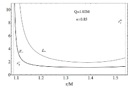
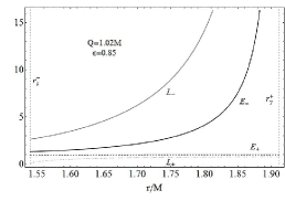
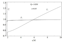
Figure 10: Class: $M<Q\leq 5/(2\sqrt{6})M$ and $\epsilon_{l}<\epsilon<\widetilde{\widetilde{\epsilon}}_{+}$. Parameter choice: $Q=1.02M$ and $\epsilon=0.85$. Then $\epsilon_{l}=0.806548$, $\widetilde{\widetilde{\epsilon}}_{+}=0.914942$, $r_{s}^{+}=1.53979M$, $r_{\gamma}^{-}=1.08866M$, and $r_{\gamma}^{+}=1.91134M$. Circular orbits exist with angular momentum $L=L_{+}$ (gray curves) and energy $E=E_{+}$ (black curves) in $r_{\gamma}^{-}<r<r_{s}^{+}$ (left plot); $L=L_{\pm}$ in $r_{s}^{+}\leq r<r_{\gamma}^{+}$ (center plot); and $L=L^{-}$ in $r\geq r_{\gamma}^{+}$ (right plot).

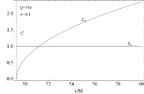
Figure 23: Class:$0<\epsilon<M/Q$ and $Q>\sqrt{9/8}M$. Parameter choice: $Q=5M$ and $\epsilon=0.1$. Then $M/Q=0.2$ and $r_{s}^{+}=49.2481M$. Circular orbits exist with angular momentum $L=L^{-}$ (gray curve) and energy $E=E^{-}$ (black curve) in $r>r_{s}^{+}$ and $L=0$ at $r=r_{s}^{+}$.

Appendix B Behavior of the angular momentum and energy of negative test charges

References

- (1) Ruffini R 1972 On the Energetics of Black Holes, Le Astres Occlus (Les Houches).
- (2) N. A. Sharp, Gen. Relativ. Grav. 10, 659 (1979).
- (3) V. P. Frolov and I. D. Novikov, Black hole physics, basic concepts and new developments (Springer, Berlin, 1998).
- (4) D. Pugliese, H. Quevedo and R. Ruffini, Phys. Rev. D 88, 2 024042 (2013).
- (5) A. F. Zakharov, Phys. Rev. D 90, 6 062007 (2014).
- (6) M. Blaschke and Z. Stuchl k, Phys. Rev. D 94, 8, 086006 (2016).
- (7) J. Kovar, P. Slany, C. Cremaschini, Z. Stuchlik, V. Karas and A. Trova, Phys. Rev. D 90, 4 044029 (2014).
- (8) B. Toshmatov, A. Abdujabbarov, B. Ahmedov and Z. Stuchl k, Astrophys. Space Sci. 357, 1 41 (2015).
- (9) Z. Stuchlik and J. Schee, Int. J. Mod. Phys. D 24, 02 1550020 (2014).
- (10) S. Beheshti and E. Gasperin, Phys. Rev. D 94, 2 024015 (2016).
- (11) Z. Stuchlik and M. Kolos, Eur. Phys. J. C 76, 1 32 (2016).
- (12) A. Tursunov, Z. Stuchlik and M. Kolos, Phys. Rev. D 93, 8 084012 (2016).
- (13) J. Kovar, P. Slany, C. Cremaschini, Z. Stuchlik, V. Karas and A. Trova, Phys. Rev. D 93, 12 124055 (2016).
- (14) D. Pugliese, G. Montani and M. G. Bernardini, Mon. Not. Roy. Astron. Soc. 428, 2 952 (2013).
- (15) D. Pugliese and Z. Stuchl k, Astrophys. J. Suppl. 221, 25 (2015).
- (16) M. A. Abramowicz, P. C. Fragile, Living Rev. Relativity 16, 1 (2013).
- (17) D. Pugliese and J. A. V. Kroon, Gen. Rel. Grav. 44, 2785 (2012).
- (18) D. Pugliese and J. A. Valiente Kroon, Gen. Rel. Grav. 48, 6 74 (2016).
- (19) D. Pugliese, H. Quevedo, J. A. Rueda H. and R. Ruffini, Phys. Rev. D 88, 024053 (2013).
- (20) R. Belvedere, D. Pugliese, J. A. Rueda, R. Ruffini and S. S. Xue, Nucl. Phys. A 883, 1 (2012).
- (21) D. Pugliese, H. Quevedo, R. Ruffini. Phys. Rev. D 83, 104052 (2011).
- (22) P. Pradhan and P. Majumdar, Phys. Lett. A 375, 474 (2011).
- (23) V. D. Gladush and M. V. Galadgyi, Gen. Rel. Grav. 43, 1347-1363 (2011).
- (24) P. S. Joshi Gravitational Collapse and Spacetime Singularities (Cambr. Univ. Press, Cambr.) (2007).
- (25) M. Patil and P. S. Joshi, Kimura, M. K. Nakao, Phys. Rev. D 86, 084023 (2012).
- (26) V. Balek, J. Bicak, Z. Stuchlik, Bull. Astron. Inst. Czechosl 40, Publishing House of the Czechoslovak Academy of Sciences, 133-165 (1989).
- (27) J. Bicak, V. Balek, Z. Stuchlik, Bull. Astron. Inst. Czechosl 40, 2 , Publishing House of the Czechoslovak Academy of Sciences, 65-92 (1989).
- (28) Z. Stuchlik, G. Bao, Gen. Rel. Grav. 24, 9, 945-957 (1992)
- (29) B. Giacomazzo, L. Rezzolla and N. Stergioulas, Phys. Rev. D 84, 024022 (2011).
- (30) J. Bicak, Lect. Notes Phys. 540, 1 (2000).
- (31) S. Chandrasekhar, The Mathematical Theory of Black Holes (Clarendon Press, Oxford and Oxford University Press, New York) (1983).
- (32) J. Levin and G. Perez-Giz, Phys. Rev. D. 77, 103005 (2008).
- (33) N. Bilic, PoS P2GC 004, (2006).
- (34) D. Pugliese, H. Quevedo, R. Ruffini, Phys. Rev. D 83, 2 (2011).
- (35) D. Pugliese, H. Quevedo and R. Ruffini, Circular motion in Reissner-Nordstróm spacetime Preprint gr-qc/1003.2687 (2010).
- (36) K. S. Virbhadra and G. F. R. Ellis, Phys. Rev. D 65, 103004 (2002).
- (37) K. S. Virbhadra and C. R. Keeton, Phys. Rev. D 77, 124014 (2008).
- (38) M. P. Dabrowski and J. Osarczuk, Astroph. Space Sci. 229, 139 (1995).
- (39) M. P. Dabrowski and I. Prochnicka, Phys. Rev. D 66, 043508 (2002).
- (40) D. Pugliese and H. Quevedo, Eur. Phys. J. C 75, 5, 234 (2015).
- (41) D. Pugliese and H. Quevedo, to be submitted.
- (42) D. Pugliese, H. Quevedo and R. Ruffini, Phys. Rev. D 84, 044030 (2011).
- (43) S. Aretakis, Annales Henri Poincare 12, 1491 (2011). -
- (44) J. Lucietti, K. Murata, H. S. Reall and N. Tanahashi, JHEP 1303, 035 (2013).
- (45) S. Aretakis, Commun. Math. Phys. 307, 17 (2011).
- (46) S. Aretakis, arXiv:1006.0283 [math.AP].
- (47) S. Dain and G. Dotti, Class. Quant. Grav. 30, 055011 (2013).
- (48) N. Andersson and H. Onozawa, Phys. Rev. D 54, 7470 (1996).
- (49) V. E. Hubeny, Phys. Rev. D 59, 064013 (1999).
- (50) J. Bicak, Phys. Lett. A 64, 279 (1977).
- (51) P. Hajicek, Nucl. Phys. B 185, 254 (1981).
- (52) P. C. Aichelburg, R. Guven, Phys. Rev. D 27, 456 (1983).
- (53) S. Ray, and B. Das, Mon. Not. R. Astron. Soc. 349, 1331-1334 (2004).
- (54) Z. Stuchlik, S. Hledik, acta physica slovaca 52, 5 363-407 (2002).
- (55) D. G. Boulware, Phys. Rev. D 8, 2363 (1973).
- (56) Ya. B. Zeldovich, I. D. Novikov, Relativistic Astrophysics 1: Stars and Relativity, The University of Chicago Press, Chicago (1971) .
- (57) J. Bicak, L. Dvorak, Phys. Rev. D 22, 2933 (1980).
- (58) V. Cardoso, C. F. B. Macedo, P. Pani and V. Ferrari, JCAP 1605, 05 054 (2016).
- (59) J. Schee and Z. Stuchlik, Int. J. Mod. Phys. D 18, 983 (2009).
- (60) Z. Stuchlik and A. Kotrlova, Gen. Rel. Grav. 41, 1305 (2009).
- (61) Z. Stuchl k and J. Schee, Int. J. Mod. Phys. D 24, 02, 1550020 (2014).
- (62) J. Schee and Z. Stuchlik, JCAP 1506, 048 (2015)