Modeling double slit interference via anomalous diffusion: independently variable slit widths

Abstract

Based on a re-formulation of the classical explanation of quantum mechanical Gaussian dispersion (Grössing et al. 2010 Groessing.2010emergence ) as well as interference of two Gaussians (Grössing et al. 2012 Groessing.2012doubleslit ), we present a new and more practical way of their simulation. The quantum mechanical “decay of the wave packet” can be described by anomalous sub-quantum diffusion with a specific diffusivity varying in time due to a particle’s changing thermal environment. In a simulation of the double-slit experiment with different slit widths, the phase with this new approach can be implemented as a local quantity. We describe the conditions of the diffusivity and, by connecting to wave mechanics, we compute the exact quantum mechanical intensity distributions, as well as the corresponding trajectory distributions according to the velocity field of two Gaussian wave packets emerging from a double-slit. We also calculate probability density current distributions, including situations where phase shifters affect a single slit’s current, and provide computer simulations thereof.

1 Introduction

In reference Groessing.2010emergence we presented a classical model for the explanation of quantum mechanical dispersion of a free Gaussian wave packet. In accordance with the classical model, we shall now relate it more directly to a “double solution” analogy gleaned from Couder.2012probabilities . For, as is shown, e.g., in Holland.1993 ; Elze.2011general , one can construct various forms of classical analogies to quantum mechanical Gaussian dispersion. Originally, the expression of a “double solution” refers to an early idea of DeBroglie.1960book to model quantum behavior by a two-fold process, i.e., by a the movement of a hypothetical point-like “singularity solution” of the Schrödinger equation, and by the evolution of the usual wave function that would provide the empirically confirmed statistical predictions. Recently, Couder.2012probabilities used this ansatz to describe the behaviors of their “bouncer”- (or “walker”-) droplets: On an individual level, one observes particles surrounded by circular waves they emit through the phase-coupling with an oscillating bath, which provides, on a statistical level, the emergent outcome in close analogy to quantum mechanical behavior (like, e.g., diffraction or double-slit interference). The simulation of interference in the double-slit experiment was in Groessing.2012doubleslit easily achieved by assuming the simple case where the two slits have equal aperture. Instead, in this paper, we discard that simplification and show in a more detailed analysis that one can i) find a formulation applicable to independently variable slit widths, and ii) provide computer simulations thereof.

2 From classical phase-space distributions to quantum mechanical dispersion

In the context of the double solution idea, which is related to correlations on a statistical level between individual uncorrelated particle positions $x$ and momenta $p$, respectively, we consider the free Liouville equation

$$\frac{\partial f}{\partial t}+\sum_{i=1}^{3}\frac{p_{i}}{m}\frac{\partial f}{\partial x_{i}}-\sum_{i=1}^{3}\frac{\partial V}{\partial x_{i}}\frac{\partial f}{\partial p_{i}}=0$$ (2.1)

with potential $V$ and mass $m$. For simplicity, we restrict ourselves to the 1-dimensional space coordinate $x$ further on. Liouville’s equation (2.1) implies the spatial conservation law and has the property that precise knowledge of initial conditions is not lost in the course of time. That is, it provides a phase-space distribution $f\left(x,p,t\right)$ that shows the emergence of correlations between $x$ and $p$ from an initially uncorrelated product function of non-spreading (“classical”) Gaussian position distributions as well as momentum distributions,

$$f_{0}\left(x,p\right)=\frac{1}{2\pi\sigma_{0}\pi_{0}}\exp\left\{-\frac{x^{2}}{2\sigma_{0}^{2}}\right\}\exp\left\{-\frac{p^{2}}{2\pi_{0}^{2}}\right\},$$ (2.2)

where $\sigma_{0}$ is the initial space deviation, i.e., $\sigma_{0}=\sigma(t=0)$, and $\pi_{0}:=mu_{0}$ is the momentum deviation. Then the phase-space distribution reads as

$$f\left(x,p,t\right)=\frac{1}{2\pi\sigma_{0}mu_{0}}\exp\left\{-\frac{\left(x-pt/m\right)^{2}}{2\sigma_{0}^{2}}\right\}\exp\left\{-\frac{p^{2}}{2m^{2}u_{0}^{2}}\right\}.$$ (2.3)

The above-mentioned correlations between $x$ and $p$ emerge when one considers the probability density in $x$–space, which is given by the integral

$$P\left(x,t\right)=\int f\,\mathrm{d}p=\frac{1}{\sqrt{2\pi}\sigma}\exp\left\{-\frac{x^{2}}{2\sigma^{2}}\right\},$$ (2.4)

with the variance at time $t$ given by

$$\sigma^{2}=\sigma_{0}^{2}+u_{0}^{2}\,t^{2}.$$ (2.5)

In other words, the distribution (2.4) describing a spreading Gaussian is obtained from a continuous set of classical, non-spreading, Gaussian position distributions whose momenta also have a non-spreading Gaussian distributions. One thus obtains the exact quantum mechanical dispersion formula for a Gaussian, as we have obtained also previously from our classical ansatz by relating different kinetic energy terms in our diffusion model Groessing.2010emergence . For confirmation with respect to that model we use the Einstein relation

$$D=\frac{\hbar}{2m}\,,$$ (2.6)

with the reduced Planck constant $\hbar=h/(2\pi)$ and $m$ being the particle’s mass, and we note that with (2.4), $\nabla P=\frac{\partial}{\partial x}P=-\frac{x}{\sigma^{2}}P$ and the usual definition of the “osmotic” velocity $u$ one obtains

$$u=u(x,t)=-D\frac{\nabla P}{P}=\frac{xD}{\sigma^{2}}\,.$$ (2.7)

For the average initial value we find

$$u_{0}:=\left.\vphantom{\int}\overline{u}\right|_{t=0}=u(\sigma_{0},0)=\frac{D}{\sigma_{0}}\,,$$ (2.8)

which turns out to be the same as the initial velocity at position $x=\sigma_{0}$ at $t=0$. This is a characteristic value for Gaussians, which we simply called “initial velocity” in our recent papers. It corresponds exactly to the velocity $u$ at starting time $t=0$ at the trajectory that has distance $\xi(0)=\pm\sigma_{0}$ from the maximum of the Gaussian (Fig. 3.1). With Eq. (2.8) one can rewrite Eq. (2.5) in the more familiar form

$$\sigma^{2}=\sigma_{0}^{2}\left(1+\frac{D^{2}t^{2}}{\sigma_{0}^{4}}\right).$$ (2.9)

Note also that by using the Einstein relation (2.6) the norm in (2.3) becomes the invariant expression

$$\frac{1}{2\pi\sigma_{0}mu_{0}}=\frac{1}{2\pi mD}=\frac{2}{h}$$ (2.10)

reflecting the “exact uncertainty relation” Hall.2002schrodinger .

3 Spreading of the wave packet due to a path excitation field

We note that $\sigma/\sigma_{0}$ is a spreading ratio for the wave packet independent of $x$. This functional relationship is thus not only valid for the particular point $\xi(t)=\sigma(t)$, but for all $x$ of the Gaussian. Therefore, one can generalize (2.9) for all $x$, i.e.,

$$\xi(t)=\xi(0)\frac{\sigma}{\sigma_{0}},\qquad\text{where }\quad\frac{\sigma}{\sigma_{0}}=\sqrt{1+\frac{D^{2}t^{2}}{\sigma_{0}^{4}}}\;.$$ (3.1)

In other words, one derives also the time-invariant ratio for the spreading

$$\frac{\xi(t)}{\sigma}=\frac{\xi(0)}{\sigma_{0}}=\text{const.}$$ (3.2)

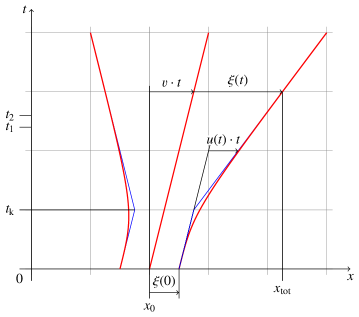
Figure 3.1: Bohm-type trajectories for a quantum particle with initial Gaussian distribution exhibiting the characteristics of ballistic diffusion

In Fig. 3.1 the spreading according to Eq. (3.1) is sketched. We can now try to implement our previous assumption that the “bouncer” particle is phase locked with its nonlocal diffusion wave field such that the Gaussian describing the diffusion process has long undulatory tails representing the locking in with the undulations of the zero-point field. In other words, we can now re-consider our classical simulations of Gaussian dispersion and double slit interference Groessing.2012doubleslit , respectively, by constructing from (2.4) a description of our “path excitation field” via the introduction of the amplitude $R$ as product of a Gaussian (at rest in the $x$–direction) and a plane wave (in the $y$–direction),

$$R\left(x,t\right)=\left(2\pi\sigma^{2}\right)^{-1/4}\exp\left\{-\frac{x^{2}}{4\sigma^{2}}\right\}\cos\left(k_{y}y\right).$$ (3.3)

The product (3.3) is factorisable for all $t$ into $x$– and $y$–dependent functions, due to the motion in the $y$–direction by $y\left(t\right)=\hbar kt/m$. According to our principle of path excitation Groessing.2012doubleslit , we deal with a single, classical particle of velocity $v=p/m$ following the propagations of waves of equal amplitude $R$ comprising a wave-like thermal bath that permanently provides some momentum fluctuations $\delta p$.

The latter are reflected in Eq. (2.9) via the r.m.s. deviation $\sigma(t)$ from the classical path. In other words, one has to do with a wave packet with an overall uniform velocity $v$, where the position $x_{0}=vt$ moves like a free classical particle, as indicated in Fig. 3.1. As the packet spreads according to Eq. (2.9), $\xi(t)$ describes the result of the motion along a trajectory of a point of this packet that was initially at $\xi(0)$. The smaller the initial value of $\left|\xi(0)\right|$, i.e., the distance from $x_{0}$ of the center point of the packet, the slower said spreading takes place. In our model picture, this is easy to understand: For a particle exactly at the center of the packet, $x_{{\rm tot}}=x_{0}\Leftrightarrow\xi(0)=0$ , the momentum contributions from the “heated up” environment on average cancel each other for symmetry reasons. However, the further off a particle is from that center, the stronger this symmetry will be broken, i.e., leading to a position-dependent net acceleration or deceleration, respectively, or, in effect, to the “decay of the wave packet”. The actual decay of the wave packet starts, roughly spoken, at a time $t_{{\rm k}}$, indicated by a “kink” in Fig. 3.1 which is due to the squared time-behavior in Eq. (2.9).

From Fig. 3.1 we find $x_{{\rm tot}}=x_{0}+v(t)t+\xi(t)$ and $\xi(t)=\xi(0)+u(t)t.$ Without loss of generality we set $v={\rm const.}$ and $x_{0}=0$ further on. With the use of Eq. (3.1) we obtain

$$x_{{\rm tot}}(t)=vt+\xi(t)=vt+\xi(0)\frac{\sigma}{\sigma_{0}}=vt+\xi(0)\sqrt{1+\frac{u_{0}^{2}t^{2}}{\sigma_{0}^{2}}}\;.$$ (3.4)

In our model picture, $x_{{\rm tot}}$ is the position of the “smoothed out” trajectories, i.e., those averaged over a very large number of Brownian motions.

Moreover, one can now also calculate the average total velocity field of a Gaussian wave packet as

$$v_{{\rm tot}}(t)=\frac{\,\mathrm{d}x_{{\rm tot}}(t)}{\,\mathrm{d}t}=v+\xi(0)\,\frac{u_{0}^{2}t/\sigma_{0}^{2}}{\sqrt{1+u_{0}^{2}t^{2}/\sigma_{0}^{2}}}\;,$$ (3.5)

which describes the velocity field $v_{{\rm tot}}$ of a point along a trajectory (i.e, the residue of the “path excitation field” to be explicated further below).

Finally, we derive the average total acceleration field of a Gaussian wave packet as

$$a_{{\rm tot}}(t)=\frac{\,\mathrm{d}v_{{\rm tot}}(t)}{\,\mathrm{d}t}=\xi(0)\,\frac{u_{0}^{2}/\sigma_{0}^{2}}{\sqrt{\left(1+u_{0}^{2}t^{2}/\sigma_{0}^{2}\right)^{3}}}\;,$$ (3.6)

describing the acceleration of a point along the trajectory at time $t$. Eqs. (3.4) to (3.6) allow us to calculate the quantities along a trajectory only from a given starting point, indicated by $\xi(0)$.

Actually, however, we are interested in the dynamics at any given position $(x,t)$ directly. Using

$$\xi(t)=x-vt$$ (3.7)

and Eq. (3.1) we rewrite

$$\xi(0)=\frac{x-vt}{\sqrt{1+u_{0}^{2}t^{2}/\sigma_{0}^{2}}}$$ (3.8)

which leads to the generalized fields,

$$x_{{\rm tot}}(x,t) =x,\vphantom{\intop_{0}^{0}}$$ (3.9)

$$v_{{\rm tot}}(x,t) =v+\xi(t)\,\frac{u_{0}^{2}t/\sigma_{0}^{2}}{1+u_{0}^{2}t^{2}/\sigma_{0}^{2}}=v+(x-vt)\,\frac{u_{0}^{2}t}{\sigma^{2}}\,,\vphantom{\intop_{0}^{0}}$$ (3.10)

$$a_{{\rm tot}}(x,t) =\xi(t)\,\frac{u_{0}^{2}/\sigma_{0}^{2}}{\left(1+u_{0}^{2}t^{2}/\sigma_{0}^{2}\right)^{2}}=(x-vt)\,\frac{u_{0}^{2}\sigma_{0}^{2}}{\sigma^{4}}\;,\vphantom{\intop_{0}^{0}}$$ (3.11)

which will be used in the simulations later on.

4 The derivation of $D_{{\rm t}}$

We derive a solution for a diffusion equation with a time-dependent diffusion coefficient $kt^{\alpha}$ for a generalized diffusion equation (cf. Mesa.2012classical )

$$\frac{\partial P}{\partial t}=kt^{\alpha}\frac{\partial^{2}P}{\partial x^{2}}\;,\quad\alpha>0.$$ (4.1)

Here, $t$ and $k$ denote the time and a constant factor, respectively. Inserting $P(x,t)$ of Eq. (2.4) as a solution into Eq. (4.1) yields

$$\frac{P\dot{\sigma}}{\sigma}\left(\frac{x^{2}}{\sigma^{2}}-1\right) =kt^{\alpha}\frac{P}{\sigma^{2}}\left(\frac{x^{2}}{\sigma^{2}}-1\right)\;,$$ (4.2)

and, after integration,

$$\frac{\sigma^{2}}{2} =k\frac{t^{\alpha+1}}{\alpha+1}+\frac{c_{0}}{2}\;.$$ (4.3)

Substitution of (2.9) into (4.3) yields $c_{0}=\sigma_{0}^{2}$ and

$$k\frac{2t^{\alpha+1}}{\alpha+1} =\frac{D^{2}t^{2}}{\sigma_{0}^{2}}\;,$$ (4.4)

which can only be fulfilled by $\alpha=1$, so that

$$k =\frac{D^{2}}{\sigma_{0}^{2}}\;.$$ (4.5)

The time-dependent diffusion coefficient $D_{{\rm t}}$ is with (2.8) identified as

$$D_{{\rm t}}:=\frac{D^{2}}{\sigma_{0}^{2}}\,t=u_{0}^{2}\,t=\frac{\hbar^{2}}{4m^{2}\sigma_{0}^{2}}\,t.$$ (4.6)

Finally, Eq. (4.1) reads as

$$\frac{\partial P}{\partial t} =\frac{D^{2}t}{\sigma_{0}^{2}}\,\frac{\partial^{2}P}{\partial x^{2}}$$ (4.7)

and turns out to be a ballistic diffusion equation, defined by $\alpha=1$, as the special case of an anomalous diffusion where the diffusion coefficient $D_{{\rm t}}$ grows linearly with time $t$.

Essentially, the “decay of the wave packet” thus simply results from sub-quantum diffusion with a diffusivity varying in time due to the particle’s changing thermal environment: as the heat initially concentrated in a narrow spatial domain gets gradually dispersed, so must the diffusivity of the medium change accordingly.

Now we look at the time $t_{{\rm k}}$ of the kink (Fig. 3.1). The wave packet begins to spread differently at the kink, which is, according to Eq. (3.1), obviously at that time $t=t_{{\rm k}}$ where the influence of the right term is equal to the left term under the square root and hence $D^{2}t^{2}\overset{!}{=}\sigma_{0}^{4}$ (i.e., $\sigma=\sqrt{2}\sigma_{0}$). Then we find with (4.6) that

$$D_{{\rm t}}=\frac{t}{t_{{\rm k}}}D.$$ (4.8)

As one can see, $t=t_{{\rm k}}$ is the time when $D_{{\rm t}}=D$. Note that the diffusivity $D$ is constant for all times $t$ and has to be distinguished from the diffusion coefficient $D_{{\rm t}}$. In a different approach, one could also start out with the “exact” uncertainty relation, $mu_{0}^{2}t_{{\rm k}}=\hbar/2$, with $u_{0}=D/\sigma_{0}$. This again leads to $D_{{\rm t}}=D^{2}t/\sigma_{0}^{2}=u_{0}^{2}t=t/t_{k}D$.

We recall Boltzmann’s relation $\Delta Q=2\omega_{0}\delta S$ Groessing.2008vacuum ; Groessing.2009origin between the heat applied to an oscillating system and a change in the action function $\delta S=\frac{1}{2\pi}\delta\int_{0}^{\tau}E_{{\rm kin}}\,\mathrm{d}t$, respectively, providing

$$\nabla Q=2\omega_{0}\nabla(\delta S)\;.$$ (4.9)

Here, $\delta S$ relates to the momentum fluctuation via

$$\nabla(\delta S)=\delta\mathbf{p}=:m\mathbf{u}=-\frac{\hbar}{2}\frac{\nabla P}{P}\;,$$ (4.10)

and therefore, with $P=P_{0}{\rm e}^{-\delta Q/kT_{0}}$ and $\Delta Q=kT=\hbar\omega$,

$$m\mathbf{u}=\frac{\nabla Q}{2\omega}\;.$$ (4.11)

Using the initial velocity (2.8) together with Eq. (4.8) we find

$$D_{{\rm t}}=u_{0}^{2}t=\frac{2}{\hbar}mu_{0}^{2}tD=\frac{2}{\hbar}\frac{(\delta p)^{2}}{2m}tD=\frac{2}{\hbar}\left[\delta S(t)-\delta S(0)\right]D=\frac{\Delta Q(t)}{\hbar\omega}D.$$ (4.12)

Actually, $\delta S(0)=0$, since there are no initial fluctuations. Substitution of (4.8) into (4.12) leads then to

$$D_{{\rm t}}=\frac{t}{t_{{\rm k}}}D=\frac{\Delta Q}{kT}D=-\ln\frac{P(t)}{P(0)}D=-D\left[\ln P(t)-\ln P(0)\right].$$ (4.13)

One can also derive a condition that does not require to know the diffusion coefficient at $t=0$,

$$\Delta D=D_{{\rm t}}(t_{2})-D_{{\rm t}}(t_{1})=-D\left[\ln P(t_{2})-\ln P(t_{1})\right],$$ (4.14)

by choosing two arbitrary time steps $t_{1}$ and $t_{2}$ as suggested in Fig. 3.1.

From condition (4.6) one can immediately see that

$$\frac{\partial D_{{\rm t}}}{\partial t}=\frac{D^{2}}{\sigma_{0}^{2}}=\textrm{const.}$$ (4.15)

Thus, one can also rewrite Eq. (4.14) as

$$\Delta D=D_{{\rm t}}(t_{1})+\frac{D^{2}}{\sigma_{0}^{2}}(t_{2}-t_{1}),$$ (4.16)

which is only valid for equal slit widths $x_{01}=x_{02}$ and thus $\sigma_{1}=\sigma_{2}$. In order to compute the distribution of $P(x,t)$, one starts with Eq. (4.16) and takes the local properties of the diffusivity into account. For given times $t_{1}$ and $t_{2}=t_{1}+\Delta t$ one obtains with (2.8),

$$D_{{\rm t}}(x,t_{1}) =-D\ln P(x,t_{1}),$$ (4.17)

$$D_{{\rm t}}(x,t_{2}) =-D\ln P(x,t_{2})+D_{{\rm t}}(x,t_{1}),$$ (4.18)

thereby constituting a rule to numerically compute the distribution $P(x,t)$.

5 Finite difference scheme

Starting with the ballistic diffusion equation (4.7) with time-dependent diffusivity $D_{{\rm t}}$ we use an explicit finite difference forward scheme (cf. Schwarz.2009numerische ),

$$\frac{\partial P}{\partial t} \rightarrow\frac{1}{\Delta t}\left(P[x,t+1]-P[x,t]\right),$$ (5.1)

$$\frac{\partial^{2}P}{\partial x^{2}} \rightarrow\frac{1}{\Delta x^{2}}\left(P[x+1,t]-2P[x,t]+P[x-1,t]\right),$$ (5.2)

with 1-dimensional cells. In case $D_{{\rm t}}$ is independent of $x$, the complete equation after reordering leads to

$$P[x,t+1]=P[x,t]+\frac{D[t+1]\Delta t}{\Delta x^{2}}\left\{P[x+1,t]-2P[x,t]+P[x-1,t]\right\}$$ (5.3)

with space $x$ and time $t$, and initial Gaussian distribution $P(x,0)$ with standard deviation $\sigma_{0}$.

As can be seen, calculation of a cell’s value at time $t$ only depends on cell values at the previous time. The time-dependence of the diffusion coefficient can also be calculated without any knowledge of neighboring cells. The diffusion coefficient represents the underlying physics of the current cell and is calculated for the evaluated time step $t+1$.

The stability condition for the scheme of Eq. (5.3) is that

$$\left|\frac{D_{{\rm t}}\Delta t}{\Delta x^{2}}\right|\leq\frac{1}{2}$$ (5.4)

be satisfied for all values of the cells $[x,t]$ in the domain of computation. The general procedure is that one considers each of the frozen coefficient problems arising from the scheme. The frozen coefficient problems are the constant coefficient problems obtained by fixing the coefficients at their values attained at each point in the domain of the computation (cf. Strikwerda.2004finite ). Substituting Eq. (4.6) into (5.4) leads to

$$\Delta t\leq\frac{\Delta x^{2}\sigma_{0}^{2}}{2D_{{\rm t}}^{2}t}\>.$$ (5.5)

This shows that the finite difference scheme (5.3) is suitable to solve the ballistic diffusion equation (4.7) as long as the spreading is not too big. Beyond that, the computations are no longer economically practical due to the necessarily enormous number of cells. Then, one has to replace the explicit scheme (5.3) by an implicit scheme, for example, which has less stringent restrictions on the stability conditions, but needs linear equation solvers instead. For our simulations we employed the explicit scheme introduced above as well as implicit schemes with an open source software for numerical computation, Scilab Scilab , on a standard personal computer.

6 The connection to wave mechanics: The double-slit experiments with different slit widths

For a more generalized picture, we now take a closer look at the double-slit experiment.

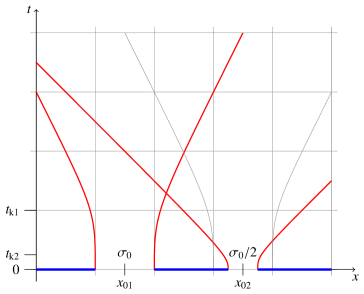
Figure 6.1: Sketch of a double-slit with two different widths and Bohm-type trajectories (and same-widths scenario indicated by gray lines)

Consider a scenario as shown in Fig. 6.1 with two slits of different widths. We assume the initial Gaussians passing through a slit have a standard deviation value matching the slit width, e.g., $\sigma_{01}=\sigma_{0}$ and $\sigma_{02}=\sigma_{0}/2$, respectively, with $\sigma_{0i}$ then being also the width of slit $i$. The resulting Bohm-type trajectories of the two decaying Gaussians are sketched in Fig. 6.1 with red lines. Thus

$$t_{{\rm k}2}=t_{{\rm k}1}/4$$ (6.1)

while the spreading is doubled (compare with the grayed out spreading of slit 2 for the case of $\sigma_{0}$ for both slits). According to Eq. (4.6), the diffusion coefficients of the two slits yield

$$D_{{\rm t},1}(t)=\frac{D^{2}t}{\sigma_{02}^{2}}\neq D_{{\rm t},2}(t)=\frac{D^{2}t}{\sigma_{01}^{2}},\quad t>0.$$ (6.2)

The advantage of Eq. (4.13) lies in it’s local fit due to its dependence on $P(x,t)$ instead on $\sigma(t)$, since the latter is just a global statistical value of too less local relevance. For the general case, we have to deal with a diffusion coefficient $D_{{\rm t}}(x,t)$ further on. The time-dependent diffusion equation reads then

$$\frac{\partial P}{\partial t}=\frac{\partial}{\partial x}\left(D_{{\rm t}}(x,t)\frac{\partial P}{\partial x}\right)\;.$$ (6.3)

We have now all the tools necessary to consider the inclusion of wave mechanics in our model. We define the phase as

$$\varphi=S/\hbar$$ (6.4)

with the general action $S$. Identifying $v_{{\rm tot}}$ of Eq. (3.10) with

$$v_{{\rm tot}}=\frac{\nabla S}{m}$$ (6.5)

we find for the action

$$S=\int mv_{{\rm tot}}(t)\,\mathrm{d}x-\int E\,\mathrm{d}t=m\int\left(v+\frac{u_{0}^{2}t}{\sigma_{0}^{2}+u_{0}^{2}t^{2}}\,\xi(t)\right)\,\mathrm{d}x-\int E\,\mathrm{d}t,$$ (6.6)

with $E$ being the system’s total energy. As $v$ does not depend on $x$ we can solve the first integral, and for the conservative case also the second integral, providing with (3.2)

$$S=mvx+\frac{mu_{0}^{2}}{2}\left(\frac{\xi(t)}{\sigma(t)}\right)^{2}t-Et=mvx+\frac{mu_{0}^{2}}{2}\left(\frac{\xi(0)}{\sigma_{0}}\right)^{2}t-Et.$$ (6.7)

Here, the action $S$ along a trajectory is given by the sum of the usual momentum-related term and a term depending on the kinetic energy, or kinetic temperature, respectively, of the “heated up” environment, weighted by a factor that solely depends on a particular trajectory indicated by the initial location $\xi(0)$ in the Gaussian.

Finally, we rewrite the phase with the help of Eqs. (6.4) and (3.7) as

$$\varphi=\frac{1}{\hbar}\left[mvx+\frac{mu_{0}^{2}}{2}\left(\frac{\xi(0)}{\sigma_{0}}\right)^{2}t-Et\right]=\frac{1}{\hbar}\left[mvx+\frac{mu_{0}^{2}}{2}\left(\frac{x-vt}{\sigma(t)}\right)^{2}t-Et\right].$$ (6.8)

The expression containing $\xi(0)$ indicates a phase $\varphi$ along a trajectory, while the r.h.s. sticks to our coordinate system and is thus the better choice to do interference calculations.

Instead of following just one Gaussian, we extend our simulation scheme to include two possible paths of a particle which eventually cross each other. For this, we use two Gaussians approaching each other. Following our earlier approach in Groessing.2012doubleslit we simulate a double-slit experiment by independent numerical computation of two Gaussian wave packets with total distribution given by

$$P_{{\rm tot}}:=P_{1}+P_{2}+2\sqrt{P_{1}P_{2}}\cos\varphi_{12}.$$ (6.9)

Since each Gaussian has its own phase (6.8) we are free to add a phase shifter $\Delta\varphi$ for one of the slits of the two-slit experiment, say slit 1, which modifies the phase to

$$\varphi{}_{1}=\frac{S_{1}}{\hbar}+\Delta\varphi$$ (6.10)

and yields for the phase difference

$$\varphi_{12}=\varphi_{2}-\varphi{}_{1}= \frac{m}{\hbar}\left[\vphantom{\intop}v_{2}(x-x_{02})-v_{1}(x-x_{01})\right]$$ (6.11)

$$+\frac{mt}{2\hbar}\left[\frac{u_{02}^{2}(x-x_{02}-v_{2}t)^{2}}{\sigma_{2}^{2}(t)}-\frac{u_{01}^{2}(x-x_{01}-v_{1}t)^{2}}{\sigma_{1}^{2}(t)}\right]-\Delta\varphi.$$

The two slits at positions $x_{01}$ and $x_{02}$ have different slit widths and hence different parameters, $\sigma_{01}$, $\sigma_{1}$, $u_{01}$ and $\sigma_{02}$, $\sigma_{2}$, $u_{02}$, respectively, as illustrated by the red trajectories in Fig. 6.1 for the example of $\sigma_{01}=\sigma_{0}$ and $\sigma_{02}=\sigma_{0}/2$, respectively. One can observe several characteristics of the averaged particle trajectories, which, just because of the averaging, are identical with the Bohmian trajectories. As one can see, the phase difference (6.11) is at any time defined for the whole domain, and hence $\varphi_{12}$ is intrinsically nonlocal.

Finally, we recall our derivation of the total average density current Groessing.2012doubleslit ; Grossing.2012quantum , i.e., the most general expression (including weights $P_{i}$) for our “path excitation field”,

$$J_{{\rm tot}}=P_{1}v_{1}+P_{2}v_{2}+\sqrt{P_{1}P_{2}}\left(v_{1}+v_{2}\right)\cos\varphi_{12}+\sqrt{P_{1}P_{2}}\left(u_{1}-u_{2}\right)\sin\varphi_{12},$$ (6.12)

where

$$v_{{\rm tot}}=\frac{J_{{\rm tot}}}{P_{{\rm tot}}}\>,$$ (6.13)

with osmotic velocities $u_{i}$ of Eq. (2.7) and total velocities $v_{i}$ of Eq. (6.5) applied to both slits, 1 and 2, and with the phases (6.11). Note that the last term on the r.h.s in Eq. (6.12) is termed “entangling current” $J_{\rm e}$ by us Groessing.2012doubleslit , which is of a genuinely “quantum” nature in that the velocities $u_{i}$ are generally entangled with the velocities $v_{i}$.

7 Simulation results

In Figs. 7.1 to 7.3, the graphical results of a classical computer simulation of the interference pattern in double-slit experiments are shown, including the trajectories. In Fig. 7.1a the maximum of the intensity is distributed along the symmetry line exactly in the middle between the two slits. Groessing.2012doubleslit

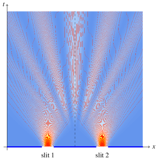
(a) equal slit widths

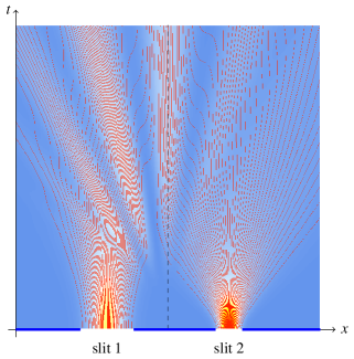
(b) $\sigma_{01}=2\sigma_{02}$

Figure 7.1: Classical computer simulation of the interference pattern with different slit widths: intensity distribution with increasing intensity from white through yellow and orange, with trajectories (red) for two Gaussian slits ($v_{x,1}=v_{x,2}=0$)

In the examplary figures, trajectories according to Eq. (6.9) for the two Gaussian slits are shown. The interference hyperbolas for the maxima characterize the regions where the phase difference $\varphi=2n\pi$, and those with the minima lie at $\varphi=(2n+1)\pi$, $n=0,\pm 1,\pm 2,\ldots$ Note in particular the “kinks” of trajectories moving from the center-oriented side of one relative maximum to cross over to join more central (relative) maxima. In our classical explanation of double slit interference, a detailed “micro-causal” account of the corresponding kinematics can be given. The trajectories are in full accordance with those obtained from the Bohmian approach, as can be seen by comparison with Holland.1993 ; Bohm.1993undivided ; Sanz.2009context ; Sanz.2012trajectory , for example.

We use the same double-slit arrangements in Figs. 7.2 and 7.3, but include a phase shifter affecting the current from slit 1, as sketched by the dashed red lines or rectangles on the left hand side, respectively. Even though the total applied phase shift is either $3\pi$ or $5\pi$ in Figs. 7.2a and 7.3a, respectively, one recognizes the effective phase difference of $\Delta\varphi_{{\rm mod}}=\Delta\varphi\mod 2\pi=\pi$ in each case, which eventually results in equal shifts of the interference fringes. By comparing with Fig. 7.1a we now observe a minimum of the resulting distribution along the central symmetry line, in full accordance with the Aharonov-Bohm effect, independently of the times $t_{1}$ and $t_{2}$ during which the shift has been applied.

To bring out the shifting of the interference fringes more clearly, we apply in Fig. 7.3 the phase shift in between the indicated times $t_{1}$ and $t_{2}$, respectively. Note that the phase shift applied only to a single slit’s current at a time $t$ when the decaying Gaussians are already overlapping (Fig. 7.3) is shown here for didactic reasons only. In this highly idealized scenario, then, one can see an illustration of the immediate effectiveness of $\Delta\varphi$ over the whole domain according to Eq. (6.11), i.e., of the nonlocality of the relative phase.

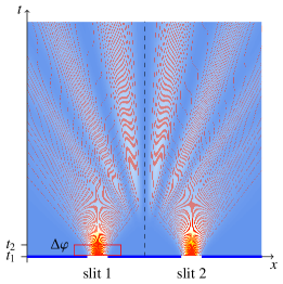
(a) Probability density $P$

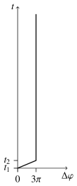
(b) Phase shift

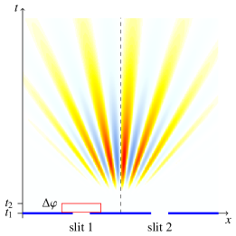
(c) Entangling current $J_{{\rm e}}$

Figure 7.2: Classical computer simulation as in Fig. 7.1a, but with additional phase shift $\Delta\varphi=3\pi$ accumulated during the time interval between $t_{1}$ and $t_{2}$ at slit 1

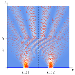
(a) Probability density $P$

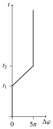
(b) Phase shift

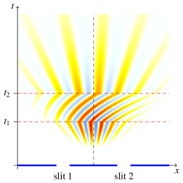
(c) Entangling current $J_{{\rm e}}$

Figure 7.3: Classical computer simulation as in Fig. 7.2, but with different times $t_{i}$ and with accumulated additional phase $\Delta\varphi=5\pi$. This results in the same distributions of $P$ and $J_{{\rm e}}$ for times $t>t_{2}$ and shows the effect of the shifting of the interference fringes more clearly than Fig. 7.2

To conclude, we have in this paper provided a detailed description of the velocity fields involved in the analytical calculations as well as the computer simulations illustrating Gaussian dispersion and interference at a double slit. We have arrived at an expression for the local value of the phase, Eq. (6.8), which made it possible also to extend our previous model to slit systems with independently variable slit widths. With the computer simulations of the latter, the nonlocal nature of the relative phase can be clearly demonstrated.

References

- (1) G. Grössing, S. Fussy, J. Mesa Pascasio, and H. Schwabl, “Emergence and collapse of quantum mechanical superposition: Orthogonality of reversible dynamics and irreversible diffusion,” Physica A 389 (2010) 4473–4484, arXiv:1004.4596 [quant-ph].
- (2) G. Grössing, S. Fussy, J. Mesa Pascasio, and H. Schwabl, “An explanation of interference effects in the double slit experiment: Classical trajectories plus ballistic diffusion caused by zero-point fluctuations,” Ann. Phys. 327 (2012) 421–437, arXiv:1106.5994 [quant-ph].
- (3) Y. Couder and E. Fort, “Probabilities and trajectories in a classical wave-particle duality,” J. Phys.: Conf. Ser. 361 (2012) 012001.
- (4) P. R. Holland, The Quantum Theory of Motion: An account of the de Broglie-Bohm causal interpretation of quantum mechanics. Cambridge University Press, Cambridge, 1993.
- (5) H. T. Elze, G. Gambarotta, and F. Vallone, “General linear dynamics - quantum, classical or hybrid,” J. Phys.: Conf. Ser. 306 (2011) 012010.
- (6) L. V. P. R. de Broglie, Non-Linear Wave Mechanics: A Causal Interpretation. Elsevier, Amsterdam, 1960.
- (7) M. J. W. Hall and M. Reginatto, “Schrödinger equation from an exact uncertainty principle,” J. Phys. A: Math. Gen. 35 (2002) 3289–3303.
- (8) J. Mesa Pascasio, S. Fussy, H. Schwabl, and G. Grössing, “Classical simulation of double slit interference via ballistic diffusion,” J. Phys.: Conf. Ser. 361 (2012) 012041, arXiv:1205.4521 [quant-ph].
- (9) G. Grössing, “The vacuum fluctuation theorem: Exact schrödinger equation via nonequilibrium thermodynamics,” Phys. Lett. A 372 (2008) 4556–4563, arXiv:0711.4954v2 [quant-ph].
- (10) G. Grössing, “On the thermodynamic origin of the quantum potential,” Physica A 388 (2009) 811–823, arXiv:0808.3539v1 [quant-ph].
- (11) H. R. Schwarz and N. Köckler, Numerische Mathematik. Vieweg+Teubner, 7 ed., 2009.
- (12) J. C. Strikwerda, Finite Difference Schemes and Partial Differential Equations. SIAM, 2 ed., 2004.
- (13) Scilab, “Free open source software for numerical computation.” Http://www.scilab.org/, 2012.
- (14) G. Grössing, S. Fussy, J. Mesa Pascasio, and H. Schwabl, “The quantum as an emergent system,” J. Phys.: Conf. Ser. 361 (2012) 012008, arXiv:1205.3393 [quant-ph].
- (15) D. Bohm and B. J. Hiley, The undivided universe: An ontological interpretation of quantum theory. Routledge, London, 1993.
- (16) A. S. Sanz and F. Borondo, “Contextuality, decoherence and quantum trajectories,” Chem. Phys. Lett. 478 (2009) 301–306, arXiv:0803.2581 [quant-ph].
- (17) A. S. Sanz and S. Miret-Artés, A Trajectory Description of Quantum Processes. I. Fundamentals. A Bohmian Perspective, vol. 850 of Lecture Notes in Physics. Springer, 2012.