Mask effects on cosmological studies with weak lensing peak statistics

Abstract

With numerical simulations, we analyze in detail how the bad data removal, i.e., the mask effect, can influence the peak statistics of the weak lensing convergence field reconstructed from the shear measurement of background galaxies. It is found that high peak fractions are systematically enhanced due to the presence of masks, the larger the masked area, the higher the enhancement. In the case that the total masked area is about $13\%$ of the survey area, the fraction of peaks with signal-to-noise ratio $\nu\geq 3$ is $\sim 11\%$ of the total number of peaks, in comparison with $\sim 7\%$ of the mask-free case in our considered cosmological model. This can have significant effects on cosmological studies with weak lensing convergence peak statistics, inducing a large bias in the parameter constraints if the effects are not taken into account properly. Even for a survey area of $9\hbox{ deg}^{2}$, the bias in $(\Omega_{m},\sigma_{8})$ is already intolerably large and close to $3\sigma$. It is noted that most of the affected peaks are close to the masked regions. Therefore excluding peaks in those regions in the peak statistics can reduce the bias effect but at the expense of losing usable survey areas. Further investigations find that the enhancement of the number of high peaks around the masked regions can be largely attributed to the fewer number of galaxies usable in the weak lensing convergence reconstruction leading to higher noise than that of the areas away from the masks. We thus develop a model in which we exclude only those very large masks with radius larger than $3\arcmin$ but keep all the other masked regions in peak counting statistics. For the remained part, we treat the areas close to and away from the masked regions separately with different noise levels. It is shown that this two-noise-level model can account for the mask effect on peak statistics very well, and the bias in cosmological parameters is significantly reduced if this model is applied in the parameter fitting.

1. Introduction

Gravitationally induced weak lensing effects have emerged as one of the most important probes in cosmological studies (e.g., Bartelmann & Schneider 2001; Albrecht et al. 2006; Amendola et al. 2012; Abate et al. 2012; Heymans et al. 2012; Erben et al. 2013; Simpson et al. 2013; Kilbinger et al. 2013). Besides the shear two-point correlation analyses, weak lensing peak statistics can provide important and complementary information especially considering that the structure formation is a nonlinear process (e.g., White et al. 2002; Hamana et al. 2004; Tang & Fan 2005; Hennawi & Spergel 2005; Marian et al. 2009; Dietrich & Hartlap 2010; Kratochvil et al. 2010; Marian et al. 2012; Hilbert et al. 2012). Current observations have proved the feasibility of detecting massive clusters from weak lensing peak identifications (e.g., Wittman et al. 2006; Gavazzi & Soucail 2007; Shan et al. 2012). Future weak lensing surveys will be able to provide a large number of peaks with high signal-to-noise ratio and therefore their statistics should expectedly be able to contribute significantly to precision cosmological studies. On the other hand, it is known that many effects can affect profoundly the weak lensing peak statistics. The complex mass distribution of clusters of galaxies and the projection effects of large-scale structures along line of sights prevent us from linking weak lensing peaks to single clusters in a simple way (e.g., Tang & Fan 2005; Yang et al. 2011; Yang et al. 2012; Hamana et al. 2012). The intrinsic ellipticities of source galaxies generate large noise that not only produces false peaks through their chance alignments (e.g., van Waerbeke 2000; Fan 2007) but also affects the true peak signals from massive clusters significantly (Fan et al., 2010, hereafter F10). Furthermore, various observational effects can also have large impacts on weak lensing peak statistics if they are not taken into account properly. The full realization of the power of weak lensing analyses in future cosmological studies relies on our thorough understandings about different systematics.

Weak lensing observations target at far away background galaxies, and bad data occurrences are unavoidable and they should be masked out carefully (e.g., Heymans et al. 2012; Erben et al. 2013). These masks can occupy $\sim 10\%$ to $\sim 20\%$ of the total survey area and result irregular survey boundaries and artificial voids in the background galaxy distribution, which in turn can affect the weak lensing analyses considerably. The mask effects on the shear power spectrum estimation and on the weak lensing Minkowski Functionals have been investigated recently (Hikage et al. 2011; Shirasaki et al. 2013). Considering weak lensing peak statistics, it involves in one way or another the reconstruction of the mass distribution from the shape measurements of background galaxies. The so called shear peak statistics is based on the aperture mass map which is the smoothed convergence field with a compensated filter (e.g., Schneider et al. 1998; Marian et al 2012). It is theoretically shown that the aperture mass at a spatial location $\boldsymbol{x}_{0}$ can be obtained by applying a suitable filter to the tangential shear field with respect to $\boldsymbol{x}_{0}$ (e.g., Schneider 1996). The filter to the tangential shear field can be derived from the compensated filter to the convergence field. Alternatively, we can apply a filter to the full shear field (not the tangential component) to obtain the smoothed shear field and then from it to reconstruct the smoothed convergence field (e.g., van Waerbeke et al. 2013). It should be noted that in this later approach, the filtering process is also applied directly to the shear field but not to the noisy convergence field reconstructed from the unsmoothed shear field. Thus the devoidness of galaxies in masked regions affects inevitably the reconstructed mass map and consequently the weak lensing peak statistics. In this paper, with numerical simulations, we perform detailed studies of the mask effect on weak lensing peak statistics and the derived cosmological parameter constraints. Specifically, we run sets of dark-matter-only N-body simulations and generate shear and convergence maps by ray-tracing. Background galaxies with intrinsic ellipticities are randomly populated and ‘observed’ ellipticities including the shear signals from simulations are then constructed for each galaxies. The masks are generated according to the mask size distribution from Shan et al. (2012), and are given spatial positions randomly in our statistical analyses. We then remove galaxies inside the masks. To obtain the weak lensing mass distribution, we adopt the above mentioned second approach to reconstruct the smoothed convergence field from the smoothed shear field obtained from the remaining galaxies. The peak statistics is analyzed and compared with the case without masks.

The rest of the paper is organized as follows. In §2, we introduce the lensing basics related to our studies, including the convergence reconstruction method. In §3, we describe the simulations and the ray-tracing method. The generation of the ‘observed galaxy ellipticities’ and the reconstruction of the convergence field from them without and with masks are presented. In §4, the theoretical model of F10 used in our peak statistical analyses is given, and its applicability is studied by comparing with the results from simulations. §5 contains the main results of our analyses of the mask effects on weak lensing peak statistics. Summary and discussions are given in §6.

2. Theoretical basics

Observationally, the weak lensing effect is mostly extracted from the shape distortion measurements of background galaxies, which is directly related to the weak lensing shear components. On the other hand, for weak lensing peak statistics, it targets at high peaks in the large-scale mass distribution, and therefore is more directly linked to the lensing convergence which is the weighted projection of the density distribution along the line of sight. The convergence and the shear are not independent quantities and all determined by the lensing potential. Thus we can derive the mass distribution from the observed shape measurements as described in the following.

Considering small source galaxies, their linear-order image distortion from the gravitational lensing effect of a single lens can be described by the Jacobian matrix given by (e.g., Schneider et al. 1992)

$$A=\bigg{(}\delta_{ij}-\frac{\partial^{2}\psi(\boldsymbol{\theta})}{\partial\theta_{i}\partial\theta_{j}}\bigg{)}=\begin{pmatrix}1-\kappa-\gamma_{1}&-\gamma_{2}\\ -\gamma_{2}&1-\kappa+\gamma_{1}\end{pmatrix},$$ (1)

where $\kappa$ is the lensing convergence and $\gamma_{1}$ and $\gamma_{2}$ are the two shear components with

$$\kappa=\frac{1}{2}\nabla^{2}\psi,\quad\gamma_{1}=\frac{1}{2}\bigg{(}\frac{\partial^{2}\psi}{\partial^{2}\theta_{1}}-\frac{\partial^{2}\psi}{\partial^{2}\theta_{2}}\bigg{)},\quad\gamma_{2}=\frac{\partial^{2}\psi}{\partial\theta_{1}\partial\theta_{2}}.$$ (2)

The lensing potential $\psi$ is determined by the surface mass density of the lens through

$$\psi(\boldsymbol{\theta})={1\over\pi}\int d^{2}\boldsymbol{\theta^{{}^{\prime}}}\frac{\Sigma(\boldsymbol{\theta^{{}^{\prime}}})}{\Sigma_{cr}}\ln|\boldsymbol{\theta}-\boldsymbol{\theta^{{}^{\prime}}}|,$$ (3)

where $\Sigma_{cr}$ is the critical surface mass density given by

$$\Sigma_{cr}={c^{2}\over 4\pi G}{D_{s}\over D_{l}D_{ls}}$$ (4)

with $D_{l},D_{s}$ and $D_{ls}$ being the angular diameter distances from the observer to the lens, to the source, and between the lens and the source. It can be seen that $\kappa=\Sigma/\Sigma_{cr}$. For weak lensing effects from large-scale structures beyond a single lens, under the Born approximation the above formulations still hold except the lensing convergence is given by, in the case of a fixed source position (e.g., Bartelmann & Schneider 2001),

$$\kappa_{eff}=\frac{3H_{0}^{2}\Omega_{m}}{2c^{2}}\int_{0}^{w}dw^{\prime}\frac{f_{K}(w^{\prime})f_{K}(w-w^{\prime})}{f_{K}(w)}\frac{\delta[f_{K}(w^{\prime})\boldsymbol{\theta},w^{\prime}]}{a(w^{\prime})},$$ (5)

where $w$ is the comoving radial distance, $f_{K}$ is the comoving angular diameter distance, $a$ is the scale factor of the universe, and $\delta$ is the density perturbation along the line of sight.

The image distortion is then described by $\kappa$ and $\gamma_{i}$ with the quantity $(\det A)^{-1}=[(1-\kappa)^{2}-|\boldsymbol{\gamma}|^{2}]^{-1}$ giving rise to the flux magnification ($|\boldsymbol{\gamma}|=(\gamma_{1}^{2}+\gamma_{2}^{2})^{1/2}$), and the eigen values of $A$ related to the axial length. Specifically, the lensing effect makes a circular source appear as an ellipse with the axial ratio of

$$\frac{a^{2}}{b^{2}}=\frac{1-\kappa-|\boldsymbol{\gamma}|}{1-\kappa+|\boldsymbol{\gamma}|}=\frac{1-|\boldsymbol{g}|}{1+|\boldsymbol{g}|},$$ (6)

where $g_{i}=\gamma_{i}/(1-\kappa)$ is named as the reduced shear component. Thus for ideally circular sources, we can obtain $\boldsymbol{g}$ by accurately measuring the shape of the sources, and further reconstruct the convergence $\kappa$ from the relation between $\kappa$ and $\gamma$, which in the Fourier space can be written as (e.g., Kaiser & Squires 1993)

$$\hat{\gamma}(\boldsymbol{l})=\pi^{-1}\hat{D}(\boldsymbol{l})\hat{\kappa}(\boldsymbol{l}),$$ (7)

where $\hat{D}$ is given by

$$\hat{D}(\boldsymbol{l})=\pi\frac{l_{1}^{2}-l_{2}^{2}+2il_{1}l_{2}}{|\boldsymbol{l}|^{2}}.$$ (8)

However, galaxies have intrinsic ellipticities. The complex ellipticity of the lensing distorted image $\boldsymbol{\epsilon}$ with $|\boldsymbol{\epsilon}|=(1-b/a)/(1+b/a)$ is then related to the intrinsic ones $\boldsymbol{\epsilon}_{s}$ by the following relation (e.g., Seitz & Schneider 1997)

$$\boldsymbol{\epsilon}=\left\{\begin{array}[]{ll}\frac{\boldsymbol{\epsilon}_{s}-\boldsymbol{g}}{1-\boldsymbol{g}^{*}\boldsymbol{\epsilon}_{s}}&\textrm{for $|{\boldsymbol{g}}|\leq 1$}\\ \\ \frac{1-\boldsymbol{g}\boldsymbol{\epsilon}_{s}^{*}}{\boldsymbol{\epsilon}_{s}^{*}-\boldsymbol{g}^{*}}&\textrm{for $|{\boldsymbol{g}}|>1$}\end{array}\right.$$ (9)

where ‘*’ represents the complex conjugation. It has been shown that the average of $\boldsymbol{\epsilon}$ gives rise to the unbiased estimate of $\boldsymbol{g}$ and $1/\boldsymbol{g}$ for $|\boldsymbol{g}|\leq 1$ and $|\boldsymbol{g}|>1$, respectively (Seitz & Schneider 1997). In the case of $\kappa\ll 1$ and $|\gamma|\ll 1$, we have $\boldsymbol{g}\approx\boldsymbol{\gamma}$.

Eq.(7) and (8) show that theoretically we can obtain the mass distribution which is related to the convergence field from the observed $\langle\boldsymbol{\epsilon}\rangle$. The aperture mass peak statistics is based on the quantity $M_{ap}(\boldsymbol{\theta})=\int d^{2}\boldsymbol{\theta}^{\prime}\kappa(\boldsymbol{\theta}^{\prime})U(|\boldsymbol{\theta}^{\prime}-\boldsymbol{\theta}|)$, where the function $U$ is a compensated filter satisfying $U(|\boldsymbol{\theta}|)=0$ for $|\boldsymbol{\theta}|>|\boldsymbol{\theta}_{0}|$ and $\int_{0}^{|\boldsymbol{\theta}_{0}|}\ |\boldsymbol{\theta}|d|\boldsymbol{\theta}|\ U(|\boldsymbol{\theta}|)=0$. From the relation between $\kappa$ and $\boldsymbol{\gamma}$, it is shown that $M_{ap}$ can be obtained directly from the tangential component of the shear with $M_{ap}(\boldsymbol{\theta})=\int d^{2}\boldsymbol{\theta}^{\prime}\gamma_{t}(\boldsymbol{\theta}^{\prime};\boldsymbol{\theta})Q(|\boldsymbol{\theta}^{\prime}|)$, where $\gamma_{t}(\boldsymbol{\theta}^{\prime};\boldsymbol{\theta})$ is the tangential shear component at $\boldsymbol{\theta}^{\prime}$ with respect to $\boldsymbol{\theta}$. The filter function $Q$ can be derived from $U$ with $Q(|\boldsymbol{\theta}|)=2/|\boldsymbol{\theta}|^{2}\int_{0}^{|\boldsymbol{\theta}|}|\boldsymbol{\theta}^{\prime}|d|\boldsymbol{\theta}^{\prime}|U(|\boldsymbol{\theta}^{\prime}|)-U(|\boldsymbol{\theta}|)$ (e.g., Schneider 1996). Therefore if the approximation $\langle\boldsymbol{\epsilon}\rangle\approx\boldsymbol{\gamma}$ is valid, one can directly obtain $M_{ap}$ from the tangential component of the observed ellipticities $\langle\boldsymbol{\epsilon}_{t}\rangle$. For peak analyses, we are interested in high peaks which are related to massive halos. In those regions, $\boldsymbol{g}\approx\boldsymbol{\gamma}$ is not a good approximation and thus $M_{ap}$ obtained from $\langle\boldsymbol{\epsilon}_{t}\rangle$ with the filter function $Q$ is not exactly equivalent to $M_{ap}$ defined through the convergence $\kappa$ with the filter function $U$. Thus there can have some complications if one wants to theoretically link $M_{ap}$ from observations to the properties of $\kappa$ due to the nonlinear relation between $\boldsymbol{g}$ and $\boldsymbol{\gamma}$.

Another approach to derive the mass distribution from the observed ellipticities $\boldsymbol{\epsilon}$ is to first obtain the smoothed field of the full $\langle\boldsymbol{\epsilon}\rangle$, and then go through the nonlinear reconstruction process to get the smoothed convergence field $\kappa$ (e.g., van Waebeke 2013). This is the approach we adopt in this paper. It is noted that the smoothing/filtering here is still applied directly to the observed ellipticities. From Eq.(9), we can construct the distortion $\boldsymbol{\delta}$ by (e.g., Schneider & Seitz 1995)

$$\boldsymbol{\delta}=\frac{2\langle\boldsymbol{\epsilon}\rangle}{1+|\langle\boldsymbol{\epsilon}\rangle|^{2}}=\frac{2\boldsymbol{g}}{1+|\boldsymbol{g}|^{2}}$$ (10)

as the observed quantity, which is independent of $|\boldsymbol{g}|\leq 1$ or $>1$. One can then solve for $\boldsymbol{\gamma}$ by

$$\boldsymbol{\gamma}=\frac{1-\kappa}{\boldsymbol{\delta}^{*}}\Big{[}1\pm\sqrt{1-|\boldsymbol{\delta}|^{2}}\Big{]},$$ (11)

where the sign is determined by $-sign[\det(A)]$. We proceed the reconstruction of the lensing convergence iteratively from the following relation

$$\kappa(\boldsymbol{\theta})=-\frac{1}{\pi}\int_{R^{2}}d^{2}\boldsymbol{\theta}^{\prime}Re[D(\boldsymbol{\theta}-\boldsymbol{\theta}^{\prime})\boldsymbol{\gamma}^{*}(\boldsymbol{\theta}^{\prime})]$$ (12)

where $D(\boldsymbol{\theta})=(\theta_{1}^{2}-\theta_{2}^{2}+2i\theta_{1}\theta_{2})/|\boldsymbol{\theta}|^{4}$. Specifically, we start by assuming $\kappa^{(0)}=0$ and $|\boldsymbol{g}|\leq 1$ everywhere, and thus (e.g., Bartelmann 1995)

$$\boldsymbol{\gamma}^{(0)}(\boldsymbol{\theta})=\frac{1-\sqrt{1-|\boldsymbol{\delta}(\boldsymbol{\theta})|^{2}}}{\boldsymbol{\delta}^{*}(\boldsymbol{\theta})}.$$ (13)

At ${n}$-th step, we obtain $\kappa^{(n)}$ from $\boldsymbol{\gamma}^{(n-1)}$ via Eq.(12) and further calculate $\boldsymbol{\gamma}^{(n)}_{test}$ from $\kappa^{(n)}$ to determine the sign of $\det(A^{(n)})$ everywhere. At $n+1$ step, we insert $\kappa^{(n)}$ into Eq. (11) to estimate $\boldsymbol{\gamma}^{(n)}$ by considering the signs of $\det(A^{(n)})$ calculated in step $n$.

In the case of $\kappa\ll 1$ and $|\boldsymbol{\gamma}|\ll 1$, we have $\langle\boldsymbol{\epsilon}\rangle=-\boldsymbol{g}\approx-\boldsymbol{\gamma}$, and thus the convergence reconstruction is a single-step linear process.

3. Simulations

To study the mask effects on weak lensing peak statistics and the corresponding cosmological parameter constraints derived from the peak analyses, we carry out sets of dark-matter-only N-body simulations in the flat $\Lambda$CDM framework. The fiducial model is taken to be $\Omega_{\mathrm{m}}=0.28$, $\Omega_{\Lambda}=0.72$, $\Omega_{\mathrm{b}}=0.046$, $h=0.7$, $\sigma_{8}=0.82$, and $n_{s}=0.96$, where $\Omega_{\mathrm{m}}$, $\Omega_{\Lambda}$, $\Omega_{\mathrm{b}}$, $h$ are the present dimensionless total matter density, energy density from the cosmological constant, baryonic matter density and the Hubble constant in units of $100\hbox{ km/s/Mpc}$, respectively. The parameter $n_{s}$ is the power index for the initial density perturbations and $\sigma_{8}$ is the root-mean-square of the linear density perturbations extrapolated to present with the top-hat smoothing scale of $8h^{-1}\hbox{Mpc}$. In order to test the applicability of our theoretical model for weak lensing peak statistics (F10), we also run four sets of simulations with different $\Omega_{m}$ and $\sigma_{8}$ near the fiducial ones. The detailed cosmological parameters for the simulations are listed in Table 1. The conventional ray tracing algorithm is adopted to calculate the deflection of light rays and the corresponding shear and convergence maps.

Table 1COSMOLOGY PARAMETERS

	fiducial	M1	M2	M3	M4
$\sigma_{8}$	0.82	0.77	0.87	0.82	0.82
$\Omega_{\mathrm{m}}$	0.28	0.28	0.28	0.25	0.31
$\Omega_{\Lambda}$	0.72	0.72	0.72	0.75	0.69
$\Omega_{\mathrm{b}}$	0.046	0.046	0.046	0.046	0.046
$h$	0.7	0.7	0.7	0.7	0.7
$n_{s}$	0.96	0.96	0.96	0.96	0.96

3.1. Base simulations

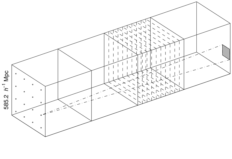
In our weak-lensing analyses, we take the source redshift $z_{s}=1$. For the fiducial cosmological model, the comoving distance to $z_{s}=1$ is approximately $2.34h^{-1}\hbox{ Gpc}$. To balance the efficiency and the resolution, we bind four independent simulations together to fill the range to $z_{s}=1$ as illustrated in Fig.1. In other words, for each set of ray-tracing calculations, we run four independent simulations with different realizations of the initial conditions. Each simulation is run in a comoving cubic box of $585.2h^{-1}\mathrm{Mpc}$ in size. Therefore in our setting, an individual simulation box occurs only once and there are no repetitious structures along line of sights. Such a design allows us to pad the simulation boxes regularly without the need of shifting and rotating to avoid the possibly multiple use of same structures in the ray tracing calculations.

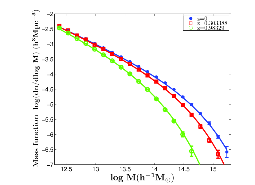
For each run, we use $640^{3}$ dark matter particles in the simulation box. The particle mass is $\sim$ $6\times 10^{10}h^{-1}\mathrm{M}_{\sun}$ for the fiducial model. The N-body code of Gadget-2 (Springel, 2005) is used to run the simulations. The initial redshift is taken to be $z=50$. The initial power spectrum is generated by CAMB (Lewis et al., 2000), and initial conditions are constructed by the code of 2LPTic (Crocce et al., 2006). The force softening length is $\sim$ 20 $h^{-1}\mathrm{kpc}$. The mass and the force resolutions should be good enough for our purpose of studies that are mainly interested in high weak-lensing peaks corresponding to massive dark matter halos with mass $M>10^{13}h^{-1}\mathrm{M}_{\sun}$ along line of sights. As a test, in Fig. 2, we show the mass functions of halos identified with the Friends-of-Friends (FoF) algorithm with the linking length of 0.18 of the average separation of dark matter particles, which is suitable for the considered cosmological model (Courtin et al., 2011). The results at redshift $z=0$ (blue symbols), $\sim 0.3$ (red symbols) and $\sim 0.98$ (green symbols) from our fiducial simulations are presented. The corresponding solid lines are the results calculated from the Sheth-Tormen mass function (ST) (Sheth & Tormen, 1999). It is seen that our simulation results agree with those from ST very well.

Figure 1.— Ray-tracing sketch.

.

For multiple-lens-plane ray tracing calculations to be described in the next subsection, we use $40$ planes corresponding to $40$ snapshots equally distributed along the comoving distance to $z=1$. Therefore there are $10$ planes for each simulation box (see Fig.1). Each plane contains particles in a slice with a comoving volume of $(58.52\times 585.2\times 585.2)\ h^{-3}\mathrm{Mpc}^{3}$. These particles are projected along the thickness of the slice into the plane with the comoving area of $(585.2\times 585.2)\ h^{-2}\mathrm{Mpc}^{2}$. The size of the simulations allows us to construct $16$ weak lensing maps of $3\times 3\deg^{2}$ each through one set of ray-tracing calculations that is based on $4$ independent runs of N-body simulations with different realizations of the initial conditions. For the fiducial model, we perform $8$ sets of ray-tracing simulations from total of $32$ runs of N-body simulations. Therefore totally we have $8\times 16=128$ weak-lensing maps of $9\deg^{2}$. For the other four cosmological models, $16$ N-body simulations are done to generate $4$ sets of ray tracing calculations, and thus $4\times 16=64$ weak-lensing maps of $9\deg^{2}$ for each model.

3.2. The multiple-lens-plane ray-tracing calculations

For the ray-tracing calculations, we follow closely the method of Hilbert et al. (2009). We use $40$ different snapshots to construct $40$ lens planes evenly distributed in the comoving distance to $z=1$. Dark matter particles within the slice of thickness of $58.52h^{-1}\mathrm{Mpc}$ around the lens plane $k$ are projected onto the plane. The two-dimensional density fluctuation field $\Sigma^{(k)}$ on a regular mesh is then constructed from the projected particle positions by the Cloud-in-Cell scheme. The potential $\hat{\psi}^{(k)}$ on the lens plane is calculated from the two-dimensional Poisson equation

$$\nabla^{2}\hat{\psi}^{(k)}=3H_{0}^{2}\Omega_{m}\frac{f_{K}^{(k)}}{a^{(k)}}\Sigma^{(k)},$$ (14)

where $f_{K}^{(k)}$ and $a^{(k)}$ are the comoving angular diameter distance to the $k$th plane and the scale factor of the universe at the epoch corresponding to the $k$th plane, and the operation $\nabla^{2}$ is taken with respect to the angular scale. We design to sample a convergence/shear map of $3\times 3\deg^{2}$ on $1024\times 1024$ pixels corresponding to $4096\times 4096$ pixels over the total $16$ maps. For the purpose of numerical accuracy, a finer mesh for 2-d density and potential calculations is needed as pointed out by Sato et al. (2009). We thus choose to sample the 2-d density and potential fields of a lens plane of $585.2\times 585.2h^{-2}\hbox{Mpc}^{2}$ on $16384\times 16384$ pixels. The resolution is then about $\sim 35.7$ $h^{-1}\mathrm{kpc}$. To suppress the Poisson noise, we further smooth the potential field with a Gaussian window function with the smoothing scale $30h^{-1}\hbox{kpc}$ (e.g, White & Vale, 2004).

Figure 2.— Mass functions for the fiducial model at different redshifts. The blue dot, red square and green circle symbols with error bars are for the simulation results at $z=0$, $z\approx 0.3$ and $z\approx 0.98$, respectively. The corresponding lines are the theoretical results calculated from the Sheth & Tormen mass function.

The deflection angle $\hat{\alpha}$ and the shear matrix $U_{ij}$ on the mesh are calculated by finite difference using the nearest neighboring grids through

$${\hat{\boldsymbol{\alpha}}}^{(k)}=\nabla\hat{\psi}^{(k)}$$ (15)

and

$$U^{(k)}_{ij}=\partial^{2}_{ij}\hat{\psi}^{(k)}.$$ (16)

To calculate the light ray position at $k$th plane, we follow the method of Hilbert et al. (2009) to use the ray positions at $k-2$ and $k-1$ planes. Specifically, we have

$$\boldsymbol{\theta}^{(k)}= \left(1-\frac{f_{K}^{(k-1)}}{f_{K}^{(k)}}\frac{f_{K}^{(k-2,k)}}{f_{K}^{(k-2,k-1)}}\right)\boldsymbol{\theta}^{(k-2)}+\frac{f_{K}^{(k-1)}}{f_{K}^{(k)}}\frac{f_{K}^{(k-2,k)}}{f_{K}^{(k-2,k-1)}}\boldsymbol{\theta}^{(k-1)}$$ (17)

$$-\frac{f_{K}^{(k-1,k)}}{f_{K}^{(k)}}{\hat{\boldsymbol{\alpha}}}^{(k-1)}(\boldsymbol{\theta}^{(k-1)}),$$

where the deflection angle ${\hat{\boldsymbol{\alpha}}}^{(k-1)}$ is calculated at the ray position $\boldsymbol{\theta}^{(k-1)}$ by interpolating from the values at grids on the mesh. We start with $\boldsymbol{\theta}^{(0)}=\boldsymbol{\theta}^{(1)}=\boldsymbol{\theta}$ with $\boldsymbol{\theta}$ being the light ray direction received by the observer. Therefore the light ray propagation can be computed iteratively.

Taking derivatives with respect to $\boldsymbol{\theta}^{(0)}$, we obtain the corresponding distortion matrix

$$A^{(k)}_{ij} =\left(1-\frac{f_{K}^{(k-1)}}{f_{K}^{(k)}}\frac{f_{K}^{(k-2,k)}}{f_{K}^{(k-2,k-1)}}\right)A^{(k-2)}_{ij}+\frac{f_{K}^{(k-1)}}{f_{K}^{(k)}}\frac{f_{K}^{(k-2,k)}}{f_{K}^{(k-2,k-1)}}A^{(k-1)}_{ij}$$ (18)

$$-\frac{f_{K}^{(k-1,k)}}{f_{K}^{(k)}}\frac{\partial{\hat{\alpha}_{i}}}{\partial\theta_{q}^{(k-1)}}\frac{\partial\theta_{q}^{(k-1)}}{\partial\theta_{j}^{(0)}}$$

$$=\left(1-\frac{f_{K}^{(k-1)}}{f_{K}^{(k)}}\frac{f_{K}^{(k-2,k)}}{f_{K}^{(k-2,k-1)}}\right)A^{(k-2)}_{ij}+\frac{f_{K}^{(k-1)}}{f_{K}^{(k)}}\frac{f_{K}^{(k-2,k)}}{f_{K}^{(k-2,k-1)}}A^{(k-1)}_{ij}$$

$$-\frac{f_{K}^{(k-1,k)}}{f_{K}^{(k)}}U^{(k-1)}_{iq}A^{(k-1)}_{qj},$$

which can also be calculated iteratively. Here again $U^{(k-1)}_{iq}$ is calculated at the ray position $\boldsymbol{\theta}^{(k-1)}$ by interpolating. With the final $A_{ij}$, we can extract the convergence $\kappa$ and the shear $\gamma_{i}$ by noting that there is an unobservable rotation angle involved in $A_{ij}$ obtained through multiple-plane ray tracing.

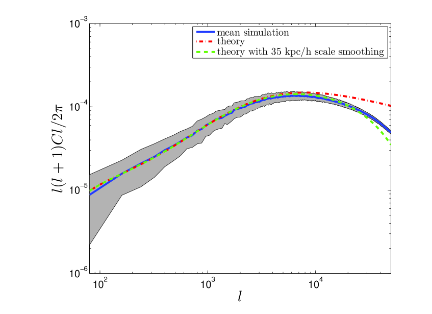
Fig. 3 presents the power spectrum calculated from the the simulated convergence maps of the fiducial model. The blue solid line is the mean result from the $128$ simulated maps of $3\times 3\deg^{2}$ with the shaded region showing the $1\sigma$ range of variation of the power spectrum from map to map. The red dash-dotted line is for the theoretical result calculated using the Limber approximation (Limber, 1954; Kaiser, 1998) given by (e.g., Bartelmann & Schneider, 2001)

$$P_{\kappa}(l)=\bigg{(}\frac{9H_{0}^{4}\Omega_{m}^{2}}{4}\bigg{)}\int_{0}^{w_{s}}dw\frac{f_{K}^{2}(w_{s}-w)}{f_{K}^{2}(w_{s})a^{2}(w)}P_{\delta}\bigg{(}\frac{l}{f_{K}(w)},w\bigg{)},$$ (19)

where $P_{\delta}$ is the power spectrum of the three-dimensional density fluctuations. We use the nonlinear $P_{\delta}$ calculated from CAMB updated according to the improved halofit model of Takahashi et al. (2012) (Lewis et al., 2000). The green dashed line is the theoretical result smoothed with a Gaussian function with the the smoothing scale of $35h^{-1}\hbox{kpc}$, approximately in accord with the simulation grid size for potential calculations. We can see that up to $l\sim 10,000$, the result from the simulations agrees with the theoretical calculations very well.

Figure 3.— The convergence power spectrum for the fiducial model. The blue solid line is for the simulation result obtained by averaging over $128$ maps. The shaded region represents the $1\sigma$ range for the variation from map to map. The red dash-dotted line is for the theoretical result calculated from Eq.(19). The green dashed line is for the smoothed theoretical result with the Gaussian smoothing scale of $35h^{-1}\mathrm{kpc}$.

3.3. Boundary problem

As discussed in Hilbert et al. (2009), a problem can rise if a fixed boundary is used to divide simulation particles into two different slices to construct the density distribution on the corresponding lens planes. It leads to artificially cut particles of a cross-boundary halo into two parts. This is particularly relevant to our studies on weak lensing peak statistics in which halos are related directly to peaks in weak lensing maps. We follow the same procedures of Hilbert et al. (2009) to deal with this boundary problem.

Specifically, in each of the $40$ snapshots, using FoF, we identify all the halos in the corresponding simulation boxes and find cross-boundary halos that have member particles on either side of a boundary. For those halos, they are included as a whole in the slice inside which their center of mass locates, and excluded completely from the other slice. Considering the possible cross-boundary motions of halos that can lead to halo double counting or missing halos, a further step adopted from Hilbert et al. (2009) is taken to avoid such a problem. For the two slices on the different sides of a boundary, if a halo is already included in the slice of the later snapshot (closer to the observer) based on its position of the center of mass, it is excluded from the other slice of the earlier snapshot even its center of mass is inside that slice at this earlier snapshot. If a halo is missed in both slices based on the position of its center of mass, it indicates that the halo moves across the boundary in the direction that is further away from the observer. In this case, we assign the halo to the slice of the earlier snapshot.

Detailed comparisons show that the differences between the convergence from the simple fixed boundary calculation and the adaptive one described above can be as large as $\sim 0.5\sigma_{0}$ for $\sigma_{0}\approx 0.02$. For halos with a typical radius of $\sim h^{-1}\mathrm{Mpc}$, about $7\%$ of them are involved in the cross-boundary problem.

In this paper, unless for comparison purposes as discussed in this subsection, all the analyses are based on the ray tracing simulations including the proper treatment of the boundary problem.

Figure 4.— Examples of convergence maps. The left one is from the base ray-tracing simulation smoothed with $\theta_{G}=1\arcmin$. The right one is the corresponding ‘g reconstruction’ convergence map from the populated galaxy catalog.

Figure 5.— The masked ‘g reconstruction’ convergence map corresponding to the right panel of Fig. 4, here the yellow patterns are the masks occurred in this case.

3.4. Fiducial reconstructed convergence maps

We follow the nonlinear reconstruction procedures described in §2 to derive the weak-lensing convergence field from background galaxy ellipticities for peak analyses.

To generate source galaxy data, for each of the $128$ simulated fields for the fiducial model, we randomly populate galaxies in angular positions at $z_{s}=1$ and assign them intrinsic ellipticities according to the following probability distribution (e.g., Bartelmann, 1995)

$$p_{s}(\epsilon_{s1},\epsilon_{s2})=\frac{\exp[-(\epsilon_{s1}^{2}+\epsilon_{s2}^{2})/\sigma_{\epsilon}^{2}]}{\pi\sigma_{\epsilon}^{2}[1-\exp(-1/\sigma_{\epsilon}^{2})]},\,\,|\epsilon_{s}|\in[0,1]$$ (20)

where $\epsilon_{s1}$ and $\epsilon_{s2}$ are the two components of the intrinsic ellipticities, $|\epsilon_{s}|=\sqrt{\epsilon_{s1}^{2}+\epsilon_{s2}^{2}}$ and the rms dispersion of $|\epsilon_{s}|$ is taken to be $\sigma_{\epsilon}=0.4$. We assume the number density of source galaxies to be $n_{g}=30\hbox{ arcmin}^{-2}$. The spatial clustering and the intrinsic alignment of source galaxies are not considered here.

The reduced shear signal $\boldsymbol{g}$ for each source galaxy is calculated from the simulated shear and convergence maps by interpolating the values on regular grids to the galaxy position. The ‘observed’ galaxy ellipticity $\boldsymbol{\epsilon}$ is then constructed according to Eq.(9).

With these galaxy data in each $3\times 3\deg^{2}$ field, we first obtain a smoothed field of $\boldsymbol{\epsilon}$ on a regular mesh of $1024\times 1024$ pixels by

$$\langle\boldsymbol{\epsilon}\rangle(\boldsymbol{\theta})=\frac{\sum_{i}W(\boldsymbol{\theta}_{i}-\boldsymbol{\theta})\boldsymbol{\epsilon}(\boldsymbol{\theta}_{i})}{\sum_{i}W(\boldsymbol{\theta}_{i}-\boldsymbol{\theta})},$$ (21)

where $\boldsymbol{\theta}$ here is for pixel position and $\boldsymbol{\theta}_{i}$ is for galaxy position. The summation is over galaxy positions. The window function $W$ is taken to be Gaussian given by

$$W(\boldsymbol{x})=\frac{1}{\pi\theta_{G}^{2}}\exp{\left(-\frac{|\boldsymbol{x}|^{2}}{\theta_{G}^{2}}\right)}.$$ (22)

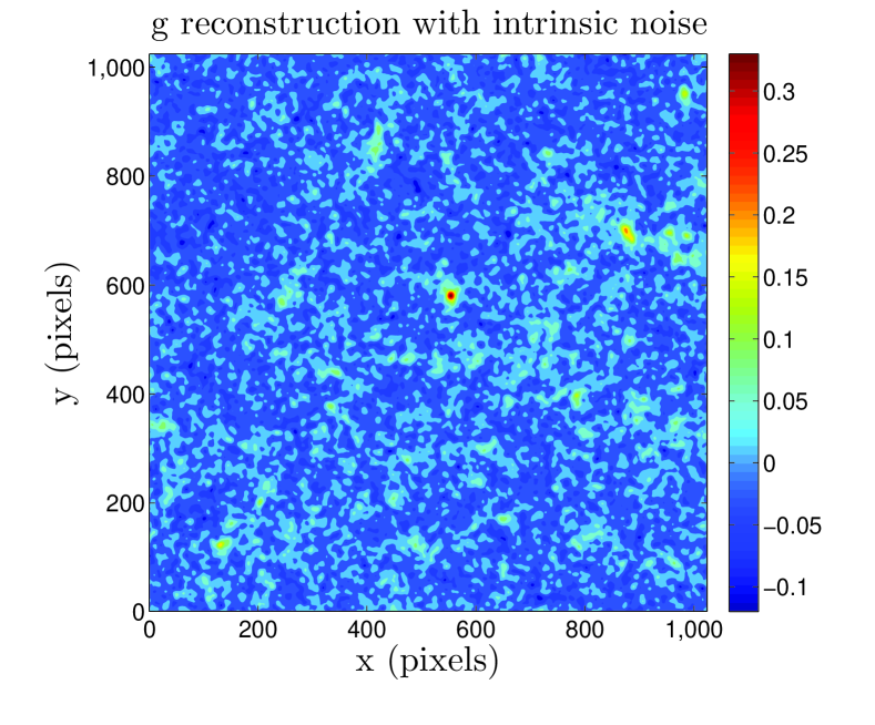
Because we are interested in high peaks that are related to massive halos, we take the smoothing scale $\theta_{G}$ to be $\theta_{G}=1\arcmin$, suitable for halos with mass about $10^{14}\hbox{ M}_{\odot}$ and above (e.g, Hamana et al., 2004). From the smoothed field $\langle\boldsymbol{\epsilon}\rangle$, the convergence reconstruction is done iteratively as described in §2. The results converge quickly with about eight iterations for the converging accuracy of $10^{-6}$, defined to be the maximum difference between the corresponding reconstructed convergence maps from two consecutive iterations. We then obtain $128$ reconstructed convergence maps, and the total area is $128\times 9=1152\deg^{2}$. We refer such maps as ‘g reconstruction’ maps. It is emphasized again that the smoothing procedure is applied directly to $\boldsymbol{\epsilon}$.

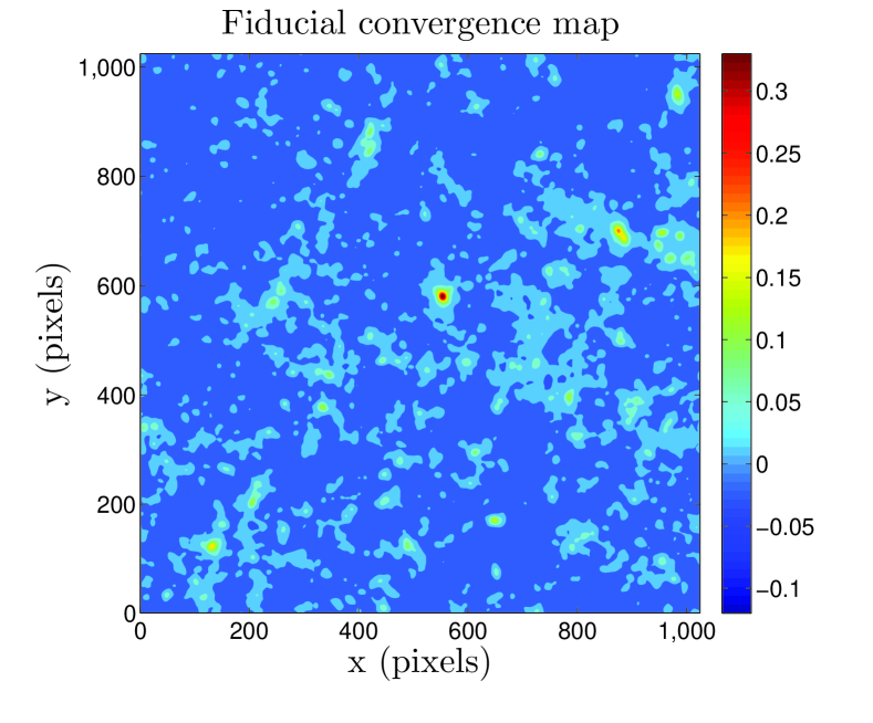
Fig. 4 shows a set of convergence maps. The left one is the pure convergence map from ray tracing simulations smoothed with a Gaussian window function with $\theta_{G}=1\hbox{ arcmin}$. The right one is the ‘g reconstruction’ map. We can see that most of the high peaks in the left map are still apparent in the right reconstructed map. However, the right one is noisy comparing to the left one due to the intrinsic ellipticities of source galaxies. The noise can affect the height of true peaks. It also generates pure noise peaks and their distribution is biased by the true mass distribution. These two noise effects have to be taken into account properly in modeling the weak lensing peak statistics (F10).

In our peak statistics analyses, we identify peaks from the reconstructed convergence maps as follows. Considering a pixel on a map of $3\times 3\deg^{2}$ ($1024\times 1024$ pixels), if its reconstructed convergence value is the highest among its nearest $8$ neighboring pixels, it is identified as a peak. To reduce the map boundary effects, we exclude the outer most $10$ pixels in each of the four sides of a map in our analyses. The signal-to-noise ratio of a peak is defined by

$$\nu=\frac{K}{\sigma_{0}}$$ (23)

where $K$ is the reconstructed convergence value of the peak, and $\sigma_{0}$ is the root-mean-square of the noise that depends on the number density of source galaxies and the smoothing scale of the window function used in obtaining the smoothed ellipticity field $\langle\boldsymbol{\epsilon}\rangle$. For a Gaussian window function used in our studies, we have (Kaiser & Squires 1993; Van Waerbeke 2000)

$$\sigma_{0}^{2}=\frac{\sigma_{\epsilon}^{2}}{2}\frac{1}{2\pi\theta_{G}^{2}n_{g}}.$$ (24)

For $\sigma_{\epsilon}=0.4$, $n_{g}=30\hbox{ arcmin}^{-2}$ and $\theta_{G}=1\arcmin$, $\sigma_{0}\approx 0.02$. In our analyses here, we consider high peaks with $\nu\geq 4$. We count peaks in $11$ bins in the range of $4.25\leq\nu\leq 9.75$ with the bin width of $0.5$. It is noted that different binnings can affect the peak abundance analyses quantitatively. Because our main focus in this paper is on the mask effects, we do not discuss the binning optimization here. We will see later that the existence of masks enhances systematically the weak-lensing peak counts in our considered signal-to-noise ratio range. This should not be changed qualitatively by different choices of peak binning. On the other hand, careful and quantitative comparisons of different binning methods for weak lensing peak analyses are desired, and will be explored in our future studies.

3.5. Mask model and convergence reconstruction with masks

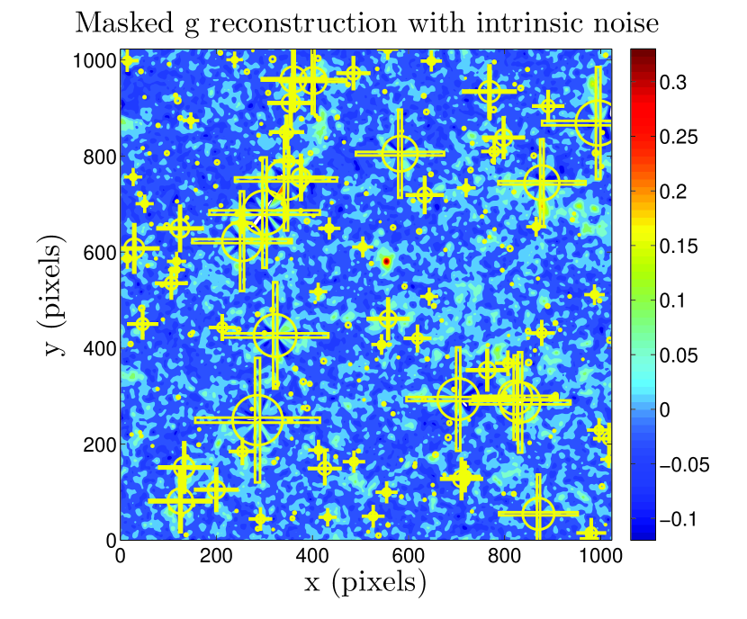
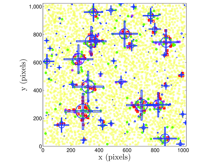
Removing bad/low quality imaging data is essential in weak lensing observational analyses. This leaves holes in the source galaxy distribution, which in turn affects the convergence reconstruction and the subsequent cosmological studies. To investigate the mask effects on weak lensing peak counts statistically, we generate mock masks by modeling the basic masks for point sources, bright saturated stars and bad pixels being circular in shape. The mask size distribution is in accord with that of CFHTLS used in Shan et al. (2012). We also add rectangle-shaped masks in both x and y directions to those circular ones with radius larger than $1\arcmin$ to mask out saturation spikes. These extra masks have a size of $0.2r\times 5r$ with $r$ being the radius of the circular mask to be added on. We populate masks randomly in each of the considered $3\times 3\hbox{ deg}^{2}$ fields. With the size distribution of Shan et al. (2012), the total number of masks in each field is set to be $N_{mask}$. We consider three cases with $N_{mask}=140,280$, and $420$, corresponding to the total masked area fraction of $\sim 7\%$, $\sim 13\%$ and $\sim 19\%$, respectively. We then remove galaxies within masks from the source galaxy catalogs generated in §3.4. With the remaining galaxies, following the reconstruction procedures we first smooth the galaxy ellipticities from Eq. (21) to get the smoothed $\langle\boldsymbol{\epsilon}\rangle$ where the summation is over the remaining galaxies, and then perform the nonlinear reconstruction to obtain the reconstructed convergence maps. Because of the removal of galaxies in masked regions, the effective number of usable galaxies in obtaining the smoothed $\langle\boldsymbol{\epsilon}\rangle$ around those area is less than the other places, causing higher noise levels. We will show later in our analyses that this non-uniform noise is mainly responsible for the mask effects on weak-lensing peak count statistics. An example of the reconstructed convergence map with masks is presented in Fig.5. The mask regions are shown in yellow.

For the fiducial model, we then have two separate sets of convergence maps reconstructed from ‘observed’ ellipticities without and with masks, respectively. Each set contains totally $128$ of $3\times 3\hbox{ deg}^{2}$ convergence maps for peak analyses.

4. The peak abundance

Our studies aim to understand the mask effects on weak-lensing peak abundances and the consequent biases on cosmological parameter constraints derived from the peak counts. To constrain cosmological parameters from weak lensing peak abundances, we need to calculate the expected peak numbers for different cosmological models. Because true high peaks in weak-lensing convergence maps correspond well to massive halos along line of sights, it is natural to relate the peak counts to the mass function of dark matter halos (e.g, Hamana et al., 2004). However, the non-spherical mass distribution of dark matter halos and the projection effects of large-scale structures can complicate the lensing signal of a halo and therefore affect the predicted peak abundance (e.g, Tang & Fan, 2005; Hamana et al., 2012). Also, the intrinsic ellipticities of source galaxies generate noise that leads to significant effects on weak-lensing peak counts from the reconstructed convergence maps as seen in Fig. 4. The easily seen noise effect is the occurrence of false peaks resulting from the chance alignments of the intrinsic ellipticities of source galaxies. Different peak identification methods have been proposed to suppress the contribution from noise peaks, such as the tomographic method, the optimal filtering method, etc. (e.g, Hennawi & Spergel, 2005; Marian et al., 2012). However, yet another effect of noise is its influence on the measured lensing signals of true peaks (e.g., Hamana et al., 2004; Yang et al., 2011; Hamana et al., 2012, F10). Therefore even we can pick out true peaks, we still need to consider the noise effect on them.

Given the complications, extensive simulation studies have been done to understand the cosmological model dependence of weak-lensing peak counts (e.g., Dietrich & Hartlap, 2010; Yang et al., 2011; Marian et al., 2012). Different phenomenological models derived from simulations have also been proposed (e.g., Marian et al., 2009; Hamana et al., 2012). Based on the theory of Gaussian random fields, Maturi et al. (2010) present an analytical model to predict the weak-lensing peak counts with relatively low signal-to-noise ratios where peaks are dominantly due to the noise from galaxy intrinsic ellipticities and the line-of-sight projection effects from large-scale structures. In F10, we develop a model for high signal-to-noise peak counts by taking into account the noise effects on the peak heights of true halos and the biased spatial distribution of noise peaks around dark matter halos.

For the analyses here, we adopt the model of F10. In §4.1, we describe the basic ingredients of the model. In §4.2, we show the model applicability by comparing with numerical simulations.

4.1. Theoretical model

Considering high peaks, the model of F10 takes into account the effects of noise from intrinsic ellipticities of source galaxies, including the noise-induced bias and the dispersion on the heights of true convergence peaks from massive halos, and the enhancement of the pure noise peak abundances due to the existence of the true mass distribution.

Figure 6.— Derivatives of the peak counts with respect to $\sigma_{8}$ (left) and $\Omega_{m}$ (right), respectively. The blue symbols with error bars are for the average results from $64$ pairs of maps. The shaded regions indicate the $1\sigma$ variation from pair to pair. The error bars show the $1\sigma$ range for the average derivatives over the $64$ pairs. The red solid line is each panel is for the result predicted from the model of F10 including the noise effect. The green lines are for the results from the theoretical model without noise.

The model assumes that the reconstructed smoothed convergence field can be written as $K_{N}=K+N$, where $K$ represents the true lensing convergence, and $N$ is for the residual noise from intrinsic ellipticities. The noise field $N$ is modeled as a Gaussian random field from the central limit theorem (e.g., van Waerbeke 2000). The model concentrates on high peaks and assumes that true peaks come from individual massive halos. Thus a considered survey area is split into halo regions and field regions. Within an individual halo region, the peak number distribution can be calculated from the Gaussian statistics of $K_{N}$ with known $K$ from the halo. Then the total number of peaks in halo regions can be obtained from the summation of the peaks in individual halo regions weighted by the halo mass function. In field regions, the number distribution of peaks is computed directly from the noise field $N$. The total surface number density of peaks can then written as

$$n_{peak}(\nu)d\nu=n_{peak}^{c}(\nu)d\nu+n_{peak}^{n}(\nu)d\nu,$$ (25)

where $\nu=K_{N}/\sigma_{0}$ is the signal-to-noise ratio of a peak. The term $n_{peak}^{c}(\nu)$ is for peaks in halo regions including both true peaks corresponding to real halos and the noise peaks within halo regions, and $n_{peak}^{n}(\nu)$ is for peaks in field regions with only noise peaks.

For $n_{peak}^{c}(\nu)$, the peak count in halo regions, it can be written as

$$n_{peak}^{c}(\nu)=\int{dz\frac{dV(z)}{dzd\Omega}}\int{dMn(M,z)f(\nu,M,z)},$$ (26)

where $dV(z)$ is the cosmological volume element at redshift z, $d\Omega$ is the solid angle element, $n(M,z)$ is the mass function of dark matter halos and,

$$f(\nu,M,z)=\int_{0}^{R_{vir}}dR(2\pi R)\hat{n}^{c}_{peak}(\nu,R,M,z)$$ (27)

gives rise to the number of peaks in the area within the virial radius of a halo of mass $M$ at redshift $z$. Here $\hat{n}^{c}_{peak}(\nu,R,M,z)$ describes the surface number density of peaks at the location of $R$ from the center of the halo, which depends on the projected density profile of dark matter halos. To calculate $\hat{n}^{c}_{peak}(\nu,R,M,z)$ in a particular halo region, we start from $K_{N}=K+N$ where $K$ is the smoothed convergence of the halo assumed to be known and to follow the Navarro-Frenk-White (NFW) mass distribution (Navarro et al., 1996, 1997). The noise field $N$ is taken to be a Gaussian random field. Therefore $K_{N}$ is also a Gaussian random field. We are interested in maxima peaks of $K_{N}$. By definition, such a maxima peak occurs in the place where the first derivatives $\partial_{i}K_{N}=0$ for $i=1,\hbox{ }2$, and the second derivative tensor $\partial_{ij}K_{N}$ should be negative definite. Thus to calculate statistically the peak abundance, we need the joint probability distribution of $K_{N}$, $\partial_{i}K_{N}$ and $\partial_{ij}K_{N}$ (e.g., Bardeen et al., 1986; Bond & Efstathiou, 1987), which, for a Gaussian field, is given by (F10)

$$p( K_{N},K^{11}_{N},K^{22}_{N},K^{12}_{N},K^{1}_{N},K^{2}_{N})\hbox{\ }dK_{N}\hbox{\ }dK^{11}_{N}\hbox{\ }dK^{22}_{N}\hbox{ }dK^{12}_{N}\hbox{ }dK^{1}_{N}\hbox{ }dK^{2}_{N}$$ (28)

$$={1\over[2\pi(1-\gamma_{N}^{2})\sigma_{0}]^{1/2}}$$

$$\times\exp\bigg{\{}-{\{(K_{N}-K)/\sigma_{0}+\gamma_{N}[(K^{11}_{N}-K^{11})+(K^{22}_{N}-K^{22})]/\sigma_{2}\}^{2}\over 2(1-\gamma_{N}^{2})}\bigg{\}}$$

$$\times{1\over 2\pi\sigma_{2}^{2}}\exp\bigg{\{}-{[(K^{11}_{N}-K^{11})-(K^{22}_{N}-K^{22})]^{2}\over 2\sigma_{2}^{2}}$$

$$-{(K^{11}_{N}-K^{11})^{2}\over\sigma_{2}^{2}}-{(K^{22}_{N}-K^{22})^{2}\over\sigma_{2}^{2}}\bigg{\}}$$

$$\times{8\over(2\pi)^{1/2}\sigma_{2}}\exp\bigg{\{}-{4(K^{12}_{N}-K^{12})^{2}\over\sigma_{2}^{2}}\bigg{\}}$$

$$\times{1\over\pi\sigma_{1}^{2}}\exp\bigg{[}-{(K^{1}_{N}-K^{1})^{2}\over\sigma_{1}^{2}}-{(K^{2}_{N}-K^{2})^{2}\over\sigma_{1}^{2}}\bigg{]}\hbox{\ }$$

$$\times dK_{N}\hbox{\ }dK^{11}_{N}\hbox{\ }dK^{22}_{N}\hbox{ }dK^{12}_{N}\hbox{ }dK^{1}_{N}\hbox{ }dK^{2}_{N},$$

where we denote $K_{N}^{i}=\partial_{i}K_{N}$ and $K_{N}^{ij}=\partial_{ij}K_{N}$, and similarly for $K^{i}$ and $K^{ij}$. Here the quantities $\sigma_{i}$ are the moments of the noise field $N$ given by (e.g., van Waerbeke, 2000)

$$\sigma_{i}^{2}=\int{d\vec{k}}\hbox{ }k^{2i}\langle|N(k)|^{2}\rangle,$$ (29)

where $N(k)$ is the Fourier transform of the noise field $N$. With the diagonalization of $(-K_{N}^{ij})$, we obtain its two eigen values $\lambda_{N1}$ and $\lambda_{N2}$ ($\lambda_{N1}\geq\lambda_{N2}$) and the rotation angle $\theta_{N}$ constrained in the range $[0,\pi]$. For maxima peaks, we require $\lambda_{N1}\geq 0$ and $\lambda_{N2}\geq 0$. We further define $x_{N}=(\lambda_{N1}+\lambda_{N2})/\sigma_{2}$ and $e_{N}=(\lambda_{N1}-\lambda_{N2})/(2\sigma_{2}x_{N})$, then the average number density of maxima peaks with a given signal-to-noise ratio $K_{N}/\sigma_{0}=\nu$ can be expressed as (e.g., Bond & Efstathiou, 1987)

$$\hat{n}^{c}_{peak}(\nu,R,M,z)= \langle\delta(K_{N}/\sigma_{0}-\nu)\delta(K^{1}_{N})\delta(K^{2}_{N})(\sigma_{2}^{2}/4)x_{N}^{2}(1-4e_{N}^{2})$$ (30)

$$\Theta(1-2e_{N})\Theta(e_{N})\rangle,$$

where the average is calculated by the probability distribution function corresponding to Eq. (28) using the variables $x_{N}$, $e_{N}$ and $\theta_{N}$ instead of $K_{N}^{11}$, $K_{N}^{22}$ and $K_{N}^{12}$. The dependence on $R$, $M$ and $z$ comes in through the halo quantities $K$, $K^{i}$ and $K^{ij}$. The step functions $\Theta(1-2e_{N})$ and $\Theta(e_{N})$ occur due to the requirements for maxima peaks. Then explicitly, we have

$$\hat{n}^{c}_{peak} (\nu,R,M,z)=\exp\bigg{[}-{(K^{1})^{2}+(K^{2})^{2}\over\sigma_{1}^{2}}\bigg{]}$$ (31)

$$\times\bigg{[}{1\over 2\pi\theta_{*}^{2}}{1\over(2\pi)^{1/2}}\bigg{]}\exp\bigg{[}-{1\over 2}\bigg{(}\nu-{K\over\sigma_{0}}\bigg{)}^{2}\bigg{]}$$

$$\times\int_{0}^{\infty}dx_{N}\bigg{\{}{1\over[2\pi(1-\gamma_{N}^{2})]^{1/2}}$$

$$\times\exp\bigg{[}-{[{x_{N}+(K^{11}+K^{22})/\sigma_{2}-\gamma_{N}(\nu_{0}-K/\sigma_{0})}]^{2}\over 2(1-\gamma_{N}^{2})}\bigg{]}$$

$$\times F(x_{N})\bigg{\}},$$

where $\theta_{*}^{2}=2\sigma_{1}^{2}/\sigma_{2}^{2}$ and $\gamma_{N}=\sigma_{1}^{2}/(\sigma_{0}\sigma_{2})$. For $K$, $K^{i}$ and $K^{ij}$ of a halo with mass $M$ at redshift $z$, we assume the spherical NFW profile for the halo and adopt the concentration-mass relation from Bhattacharya et al. (2013) given by

$$c_{vir}(M,z)=\tilde{D}(z)^{0.9}7.7\bigg{[}\frac{\delta_{c}}{\sigma(M,z)}\bigg{]}^{-0.29}.$$ (32)

Here $\tilde{D}(z)$ is the linear growth factor normalized to $z=0$ calculated with the fitting formula given by Carroll et al. (1992). The quantity $\delta_{c}$ is the linear collapse threshold at redshift $z$ computed according to Henry (2000). The quantity $\sigma(M,z)$ is the rms of the smoothed linear density fluctuations at redshift $z$ over the top-hat scale corresponding to $M$, and is calculated with the same linear power spectrum as that used in our N-body simulations from CAMB taking into account the linear growth factor at $z$.

The function $F(x_{N})$ in Eq. (31) is given by (F10)

$$F(x_{N})= \exp\bigg{[}-{(K^{11}-K^{22})^{2}\over\sigma_{2}^{2}}\bigg{]}\times$$

$$\int_{0}^{1/2}de_{N}\hbox{ }8(x_{N}^{2}e_{N})x_{N}^{2}(1-4e_{N}^{2})\exp(-4x_{N}^{2}e_{N}^{2})\times$$

$$\int_{0}^{\pi}{d\theta_{N}\over\pi}\hbox{ }\exp\bigg{[}-4x_{N}e_{N}\cos(2\theta_{N}){(K^{11}-K^{22})\over\sigma_{2}}\bigg{]}.$$

With $\hat{n}^{c}_{peak}(\nu,R,M,z)$ in Eq. (31), we can then calculate $f(\nu,M,z)$ by Eq. (27), and further $n^{c}_{peak}(\nu)$ by Eq. (26) where we adopt the Sheth-Tormen mass function in the calculations (Sheth & Tormen, 1999) .

For the field term $n_{peak}^{n}(\nu)$ in Eq. (25), it is given by

$$\begin{split}n_{peak}^{n}(\nu)=\frac{1}{d\Omega}\Big{\{}n_{ran}(\nu)\Big{[}d\Omega-\int dz\frac{dV(z)}{dz}\\ \times\int dM\,n(M,z)\,(\pi R_{vir}^{2})\Big{]}\Big{\}},\end{split}$$ (34)

where $n_{ran}(\nu)$ is the surface number density of pure noise peaks without foreground halos. It can be calculated by Eq. (31) with $K=0$, $K^{i}=0$ and $K^{ij}=0$.

Further details of the model can be found in F10.

4.2. The comparison of the model with simulations

To test the model applicability in cosmological studies, we compare the peak counts predicted from the model of F10 with simulation results in terms of their cosmological dependence. Within the flat $\Lambda$CDM framework, we concentrate on $\Omega_{m}$ and $\sigma_{8}$, the two most important parameters for weak-lensing analyses. Therefore for comparison purposes, in addition to the fiducial model runs, we also perform ray-tracing simulations for four other cosmological models with different $(\Omega_{m},\sigma_{8})$ around the fiducial values as shown in Table 1.

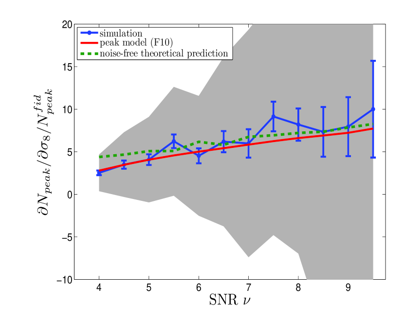
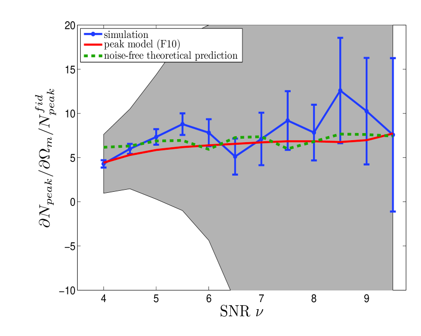
For each of the variational model, we run four sets of ray-tracing simulations and obtain totally $4\times 16=64$ weak-lensing maps each with $3\times 3\deg^{2}$. In order to suppress the cosmic variance so that to reveal the cosmological dependence of the peak counts clearly, except with different $\Omega_{m}$ or $\sigma_{8}$, each set of the simulations is done in the identical way as that of the corresponding fiducial model with matched initial conditions for each N-body run. For each of the maps, we perform the convergence reconstruction also in a way that is identical to the corresponding fiducial one using the same background galaxy catalog. With these matched reconstructed maps, the derivatives of the peak counts with respect to $\Omega_{m}$ and $\sigma_{8}$ are then analyzed separately as follows using the double-sided derivative estimator (e.g., Marian et al., 2013)

$$\frac{{\partial{N}_{peak}(\nu_{i})}}{\partial{p_{\alpha}}}|_{p_{\alpha}}=\frac{1}{M}\sum_{f=1}^{M}\frac{N_{peak}^{f}(\nu_{i},p_{\alpha}+\Delta p_{\alpha})-N_{peak}^{f}(\nu_{i},p_{\alpha}-\Delta p_{\alpha})}{2\Delta p_{\alpha}},$$ (35)

where $p_{\alpha}$ stands for the cosmological parameter we are interested in, and specifically $\Omega_{m}$ or $\sigma_{8}$ for the analyses here, $f$ is for different matched pairs of maps with the total number of pairs $M=64$, $N_{peak}^{f}(\nu_{i},p_{\alpha}\pm\Delta p_{\alpha})$ is for the number of peaks in the signal-to-noise ratio bin centered on $\nu_{i}$ with bin width of $0.5$ in the map of $3\times 3\deg^{2}$ with the cosmological parameter $p_{\alpha}\pm\Delta p_{\alpha}$ in pair $f$. The derivatives are estimated at the fiducial value $p_{\alpha}$.

The results are shown in Fig. 6, where the left and right panels are for the derivatives with respect to $\sigma_{8}$ and $\Omega_{m}$, respectively, divided by the corresponding average peak number from the fiducial model. The blue symbols with error bars are for the simulation results. The shaded regions indicate the $1\sigma$ ranges of the variations of the derivatives estimated from single pairs. The error bars show the expected errors for the values averaged over the $64$ pairs of maps. The red solid lines are the results calculated from our model F10 taking into account the noise effects, and the green dash lines are for the theoretical results without including the noise effects calculated from the halo mass function assuming spherical NFW halos (e.g., Hamana et al., 2004, F10). It is seen that within the error ranges, our model predictions (red lines) agree with the simulations results very well. Comparing the red and green lines, we can see that the two are in good accord with each other for peaks with $\nu\geq 6$. On the other hand, for peaks with $\nu\sim 4-5$, the green lines are higher than the red lines, signifying more cosmological information predicted by the green ones. This shows that the noise is important for peak counts with $\nu\sim 4-5$. It is noted that in our model F10, we only include the noise effect from intrinsic ellipticities of source galaxies, and do not consider the projection effect from line-of-sight large-scale structures and the nonspherical mass distribution for dark matter halos. While the noise is indeed the dominant source of errors, the latter two effects can also affect the peak counts to some extent, and they contain cosmological information themselves (e.g., Tang & Fan, 2005; Hamana et al., 2012). This may be related to the tendency seen in Fig. 6 that the simulation results are mildly higher than the red lines. We will explore the model improvements further in our future studies. For the current analyses, we conclude that within the error ranges, the cosmological dependence predicted by our model with the noise effect included are in very good agreements with the simulation results.

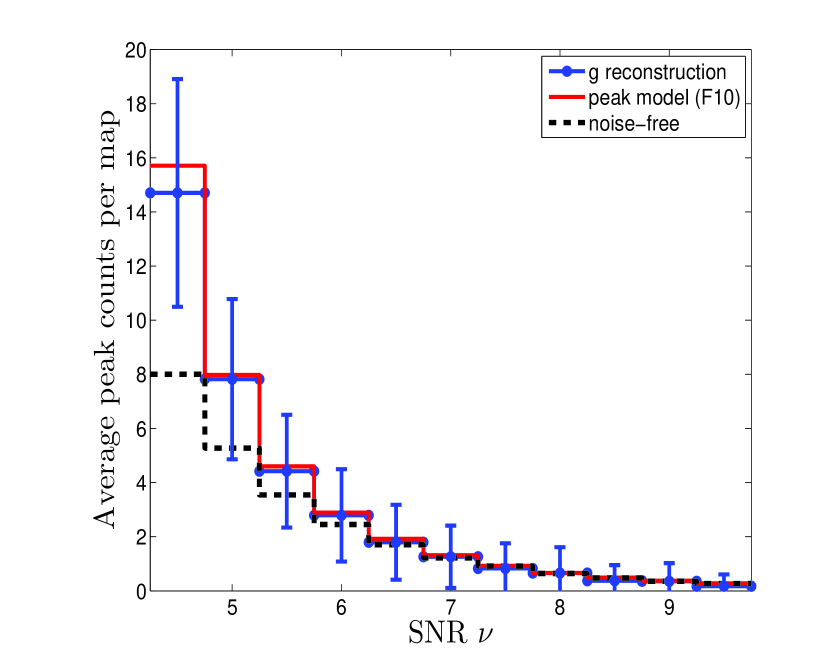
Besides the derivatives with respect to cosmological parameters, we also perform a direct comparison between peak counts from simulations and our model prediction. The results are shown in the left panel of Fig. 7. The blue histograms show the peak counts in $3\times 3\deg^{2}$ averaged over the $128$ ‘g-reconstruction’ maps for the fiducial model. The attached error bars are for the $1\sigma$ ranges of the map-to-map variations. The red histograms are our model predictions, and the black ones are for the theoretical results without including the noise effects. We can see that in the considered peak range, there is an excellent agreement between the results from our model prediction and those from simulations. The black histograms are systematically lower than the simulation results for $\nu\sim 4-6$, again demonstrating clearly the noise effect on peak counts. Therefore if this model without including the noise effect is used in cosmological parameter fitting, a significant bias can arise. On the other hand, our model F10 can expectedly give better constraints. We note again that here we use $11$ bins, linearly distributed in the considered signal-to-noise ratio range with the bin width of $0.5$, in our peak counting. Different binning methods can give rise to specifically different values of peak counts. However the systematic agreement of the trend between the blue and red histograms and the systematic differences between them and the black ones indicate that a different choice of binning should not change the results of their comparisons qualitatively. Similarly for the mask effects to be discussed in the following.

Given the good agreements within error ranges shown above, in the studies for the mask effects on weak-lensing peak counts and the consequent bias on the derived cosmological parameters, we adopt the model of F10 in the cosmological parameter fitting analyses.

Figure 7.— Left: The average numbers of peak counts per map for the fiducial model. The blue histograms with error bars are for the results from ‘g reconstruction’ maps. The red histograms are the results predicted from F10. The black histograms are for the results from the theoretical model without noise. Right: Cosmological constraints on $(\Omega_{m},\sigma_{8})$ from $\chi^{2}$ fitting for a survey of $9\deg^{2}$ from the ‘g reconstruction’ maps without masks. The contours from inside out show the $1\sigma$, $2\sigma$ and $3\sigma$ ranges, respectively. The dashed line gives more or less the degeneracy direction between $\Omega_{m}$ and $\sigma_{8}$ in terms of weak-lensing peak counts considered here.

4.3. Cosmological parameter fitting from peak counts

Shown in the previous subsection, our model including the noise effects agree well with simulation results. We then use the peak counts identified directly from reconstructed maps for cosmological studies without the need to distinguish true and false peaks. To derive cosmological parameter constraints from weak-lensing peak counts, we minimize the $\chi^{2}$ defined as follows

$$\chi_{p^{\prime}}^{2}=\boldsymbol{dN}^{(p^{\prime})}(\widehat{\boldsymbol{C}^{-1}})\boldsymbol{dN}^{(p^{\prime})}=\sum_{ij=1,...,11}dN_{i}^{(p^{\prime})}(\widehat{C_{ij}^{-1}})dN_{j}^{(p^{\prime})},$$ (36)

where $dN_{i}^{(p^{\prime})}=N_{peak}^{(p^{\prime})}(\nu_{i})-N_{peak}^{(d)}(\nu_{i})$ with $N_{peak}^{(p^{\prime})}(\nu_{i})$ being the prediction for the cosmological model $p^{\prime}$ from F10 and $N_{peak}^{(d)}(\nu_{i})$ being the ‘observed’ data for the peak count in the signal-to-noise ratio bin centered on $\nu_{i}$, and $C_{ij}$ is the covariance matrix of the peak counts including the error correlations between different $\nu$ bins. It has been shown that the direct inversion of $C_{ij}$ estimated from simulated maps leads to an biased estimate of its inverse. An unbiased estimator of the inverse covariance matrix is given by Hartlap, Simon & Schneider (2007)

$$\widehat{\boldsymbol{C}^{-1}}=\frac{R-N_{bin}-2}{R-1}(\boldsymbol{C}^{-1}),~{}~{}N_{bin}<R-2$$ (37)

where $N_{bin}$ is the number of bins used for peak counting, and R is the number of independent maps used in calculating $C_{ij}$. In our case, $N_{bin}=11$ and $R=128$. We adopt $\widehat{\boldsymbol{C}^{-1}}$ to evaluate the inverse covariance matrix during the whole analysis.

The ‘observed’ data are constructed from the simulations for the fiducial model as follows. For each of the $128$ reconstructed maps without or with masks, we identify peaks following the descriptions in §3.4. To reduce the boundary effect on peak counts, we exclude the outermost $10$ pixels in each direction in peak counting. Thus the effective area of each map is $[3(1-20/1023)]^{2}\approx 8.65\hbox{ deg}^{2}$. For each map $r$, we count peaks in each of the $11$ signal-to-noise ratio bins of width $\Delta\nu=0.5$ in the range of $4.25\leq\nu\leq 9.75$. We then calculate the mean number of peaks in each bin by averaging over the $128$ maps, and scale it back to $9\hbox{ deg}^{2}$ by multiplying a factor of $9/8.65$. These average peak counts form the ‘observed’ data $N_{peak}^{(d)}(\nu_{i})$ with $\nu_{i}=\{4.5,5.0,5.5,6.0,6.5,7.0,7.5,8.0,8.5,9.0,9.5\}$, respectively.

The covariance matrix $C_{ij}$ is also calculated from the $128$ simulated maps by

$$C_{ij}=\frac{1}{R-1}\sum_{r=1}^{R}[N^{r}_{peak}(\nu_{i})-{N}_{peak}^{(d)}(\nu_{i})][N^{r}_{peak}(\nu_{j})-{N}_{peak}^{(d)}(\nu_{j})]$$ (38)

where $r$ denotes for different maps with the total number of maps $R=128$, and $N^{r}_{peak}(\nu_{i})$ is for the peak count in the bin centered on $\nu_{i}$ from the map $r$ (scaled back to $9\deg^{2}$).

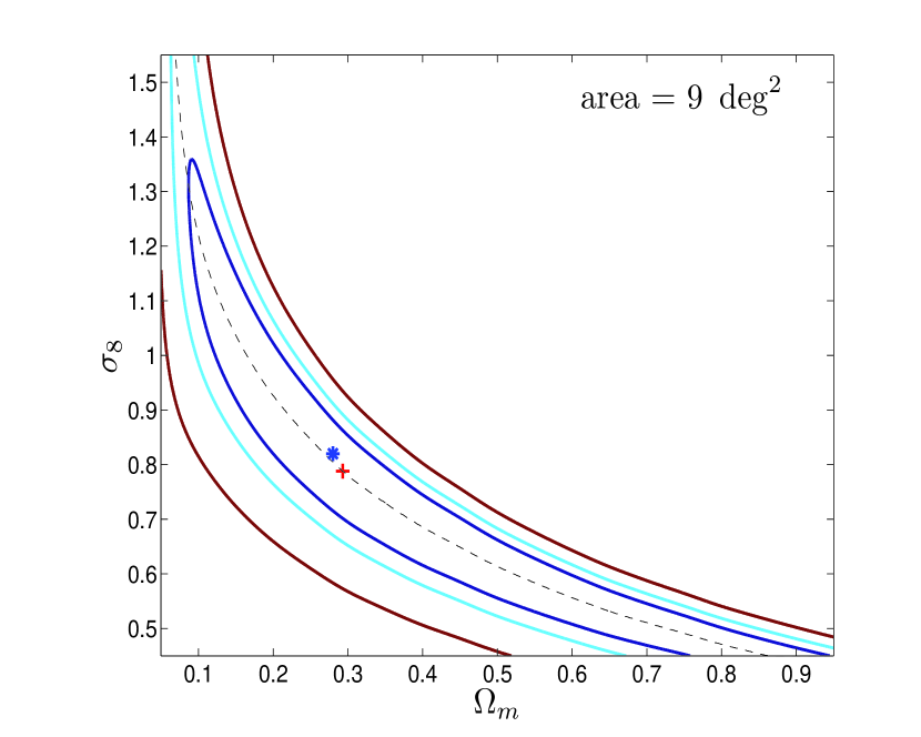
The right panel of Fig. 7 shows the fitting result of $(\Omega_{m},\sigma_{8})$ with the data obtained from the reconstructed maps for the fiducial model without masks. Here the red symbol indicates the best fit values, and the contours from inside out show the $1,2,3\sigma$ ranges, respectively. The blue symbol is for the input $(\Omega_{m},\sigma_{8})$ for the fiducial model. We see that the best fit result obtained using our model agrees with the fiducial input very well. This further demonstrates the cosmological applicability of our model within error ranges in addition to the comparisons shown in §4.2.

We now proceed to analyze the mask effects on weak-lensing peak counts and consequently on cosmological studies.

Figure 8.— The mask effects on peak positions. The left panel shows the spatial distribution of peaks in one map. The square and plus symbols are for peaks in the case with and without masks, respectively. The red, black and yellows ones are, respectively, for peaks with spatial offsets larger than $0.5\hbox{ arcmin}$, in the range of $[0.2\hbox{ arcmin},0.5\hbox{ arcmin}]$ and less than $0.2\hbox{ arcmin}$. The masks are shown in blue. The right panel is the statistical distribution of the spatial offset obtained by averaging over the $128$ pairs of maps.

Figure 9.— The peak counts distribution. The left panel shows the peak number distributions for the cases without (purple) and with (yellow) masks, respectively. The right panel shows the peak number difference between the two cases as a function of $\nu=K_{N}/\sigma_{0}$ with $\sigma_{0}=0.02$.

5. Results

5.1. Mask effects

In this section, we discuss the mask effects on weak lensing peak analyses by comparing two sets of $g$-reconstructed convergence maps with and without masks, respectively. There are totally $128$ maps for each set. For each map in the case without masks, there is a corresponding map with masks that the source galaxies are exactly the same as the other one except that the galaxies within the masked regions are discarded and the convergence reconstruction is done from the smoothed $\langle\boldsymbol{\epsilon}\rangle$ field obtained from the remaining galaxies. We then have $128$ pairs of maps that allow us to do detailed comparisons. The mask size distribution model is described in §3.5. Three cases with the total number of masks $N_{mask}=140,280$ and $420$ for each $9\hbox{ deg}^{2}$ are considered, which corresponds to the masked area fraction of $\sim 7\%,\sim 13\%$ and $\sim 19\%$, respectively. The case with $N_{mask}=280$ is taken to be our fiducial case for most of the results presented in the following.

To perform detailed comparisons for peaks in convergence maps with and without masks, we need to identify the peak correspondences between each pair of maps. This is done by peak matching. For each peak in a map from one set, we check for peaks within $3.5\hbox{ arcmin}$ in each dimension around it in its peer map from another set and define the nearest peak within this region as its partner peak. Only those pairs of peaks that are partners to each other are identified as peaks with correspondences.

The existence of masks affects the convergence reconstruction and consequently the peak properties both in their spatial location and peak height.

Figure 10.— The illustration of the spatial distribution of the affected peaks. In the left panel, the red, green and purple symbols are for Type I affect peaks, Type II affected peaks and Type II with $\nu\geq 2$, respectively. The yellow symbols are for the rest of the peaks with correspondences between the case with and without masks. The right panel shows the Type I peaks with $\nu<3.25$ in the case without masks but with the corresponding peak height shifting to $\nu>4.25$ in the case with masks (red symbols).

Figure 11.— The comparison of the peak counts between the cases with and without masks, where the blue, green and red histograms are for the cases with masks, without masks and the model prediction of F10 with a uniform noise of $\sigma_{0}=0.02$.

Figure 12.— The bias in cosmological parameter constraints due to the mask effects. The left panel shows the fitting results for the survey area of $9\hbox{ deg}^{2}$. The blue symbol is for the fiducial values and the red symbol is for the best fit with the peak counts in the case with masks as the ‘observed data’ and $\sigma_{0}=0.02$ in the model of F10. The right panel is for the results with the survey area of $150\hbox{ deg}^{2}$.

5.1.1 Spatial location

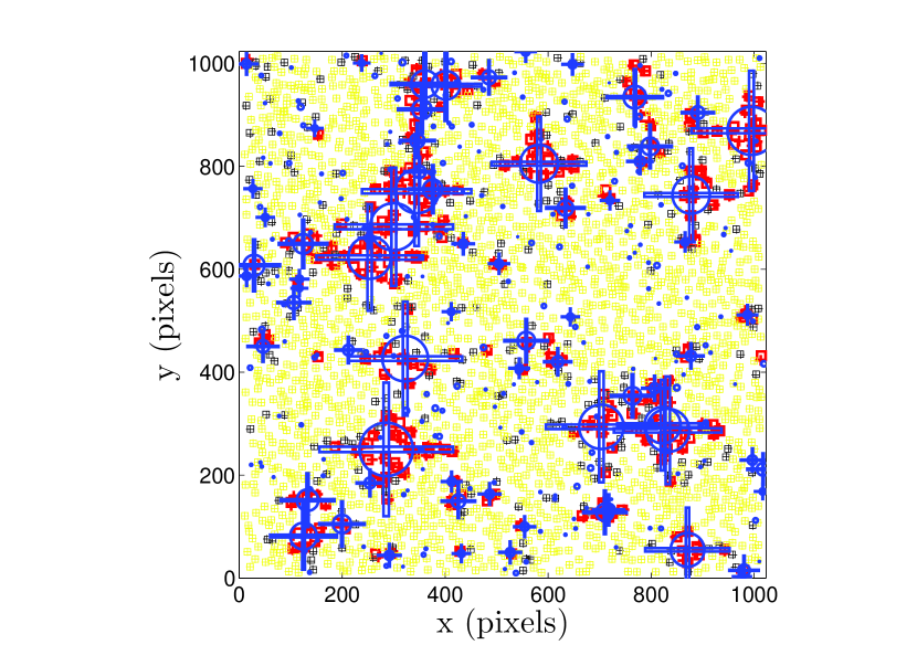
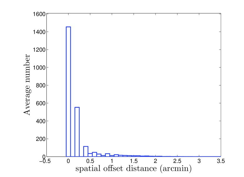
In Fig. 8 we present the mask effect on spatial positions of peaks for $N_{mask}=280$. The left panel shows an example map of the spatial distribution of peaks with correspondences. The squared and plus symbols are respectively for peaks in the cases with and without masks. The red, black and yellow ones are for the pairs of peaks with their spatial offset larger than $0.5\hbox{ arcmin}$, in the range of $[0.2,0.5]\hbox{ arcmin}$ and less than $0.2\hbox{ arcmin}$, respectively. It is seen clearly that strongly affected peaks are almost all closely associated with masks, especially large masks. In the right panel of Fig. 8, the statistical offset distribution averaged over $128$ pairs of maps is shown. There are about $40\%$ of peaks with offset larger than $0.1\hbox{ arcmin}$. The fraction with offset larger than $0.5\hbox{ arcmin}$ is $\sim 11\%$. We also notice that lower peaks are more strongly affected by masks. This offset due to mask can have significant effects on weak lensing analyses for individual clusters. For a typical weak lensing observation targeting at a particular cluster, the observed size is about $20\hbox{ arcmin}$. If there happens to be a large mask close to the central region of the cluster, the weak lensing determined center for the cluster can be considerably offsetted from its true center, which in turn can lead to large errors in the weak lensing determination of the density profile for the cluster.

5.1.2 Peak height

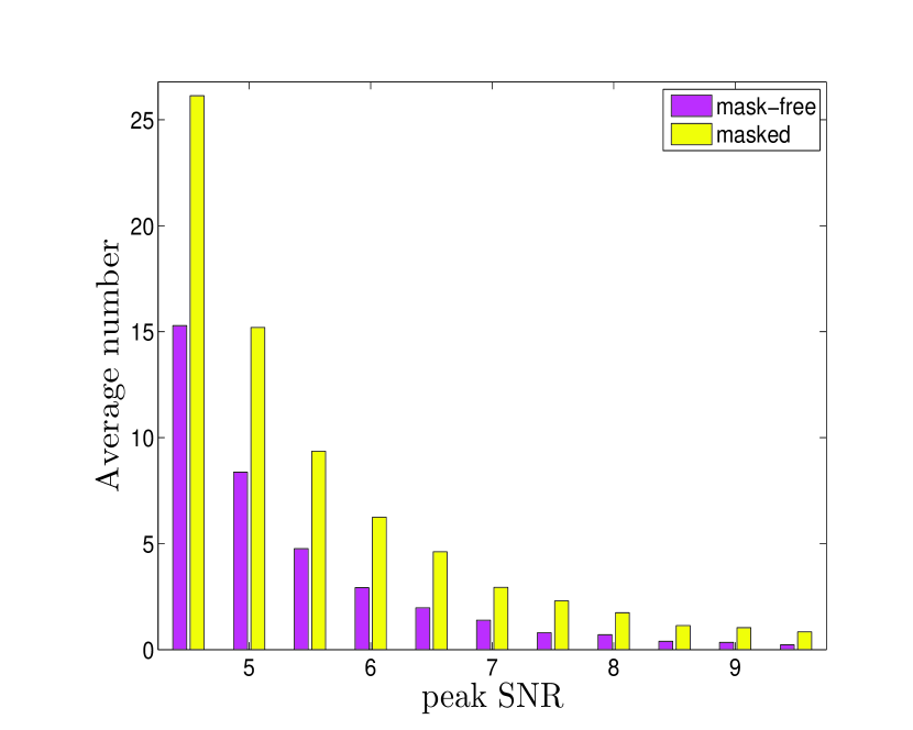
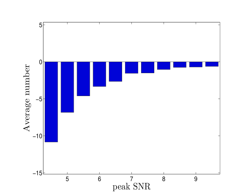
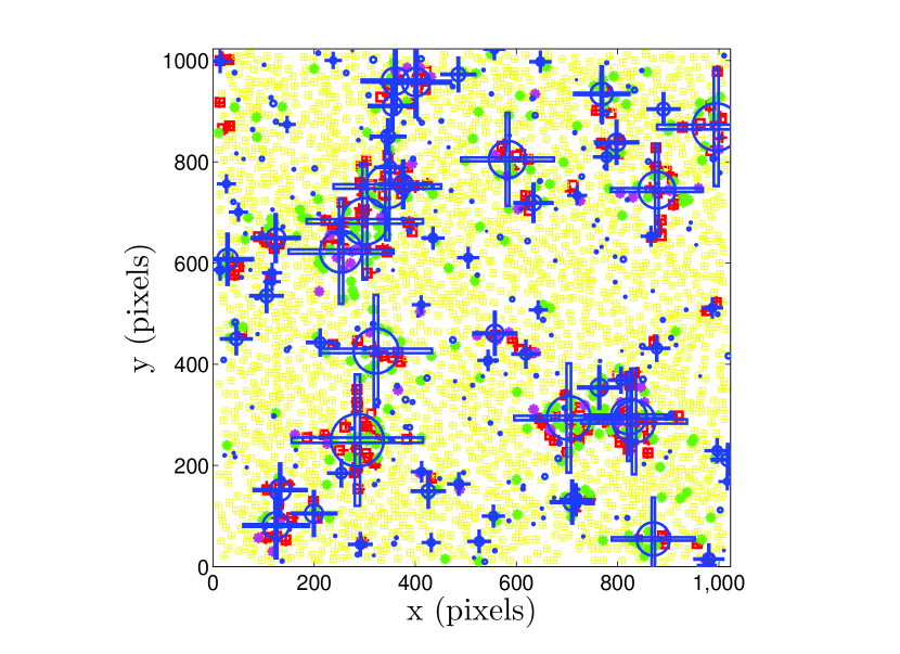
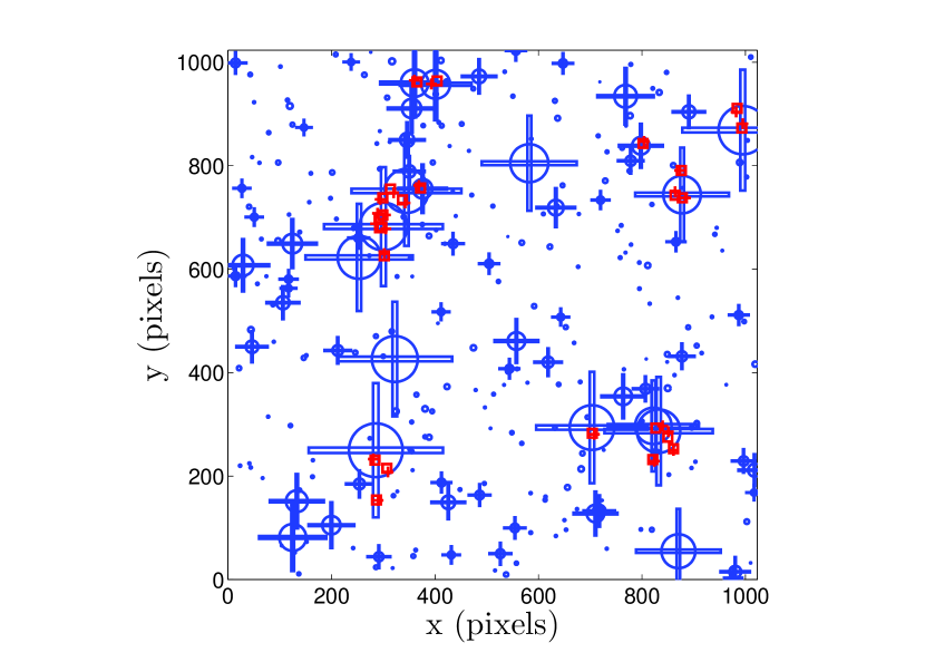
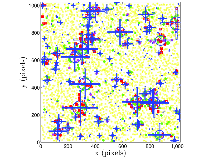
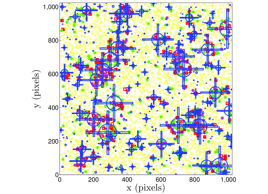
We now discuss the mask effects on peak heights. Fig. 9 shows the results, where the left panels are the peak number distribution in $9\hbox{ deg}^{2}$ averaged over $128$ maps in each case and the right panels are the peak number differences between the cases without and with masks, respectively, as a function of S/N ($\nu=K_{N}/\sigma_{0}$ with $\sigma_{0}=0.02$). It is clearly seen that the number of peaks in high signal-to-noise bins is systematically higher in the case with masks, which can expectedly affect the cosmological parameter constraints with weak lensing peak counts significantly. We further exam the correlation between the positions of the strongly affected peaks and the locations of masks. We define two types of strongly affected peaks. Type I is for peaks with their peak height difference between the cases with and without masks higher than $1\sigma$. Type II is for peaks without correspondences between the two cases. Fig. 10 presents a typical map with masks. The left panel shows the spatial distribution of peaks with squares and pluses for peaks in the cases with and without masks, respectively. The red symbols are for Type I peaks, the green symbols are for Type II peaks with the purple ones for Type II peaks with $\nu\geq 2$, and the yellows ones are for the rest. The clustering of the strongly affected peaks around large masks are apparent. The right panel shows particularly the Type I peaks with $\nu<3.25$ in the case without masks but with the corresponding peak height shifting to $\nu>4.25$ in the case with masks. It is found that they all trace large masks. It is these high Type I peaks that can affect profoundly the cosmological parameter constraints.

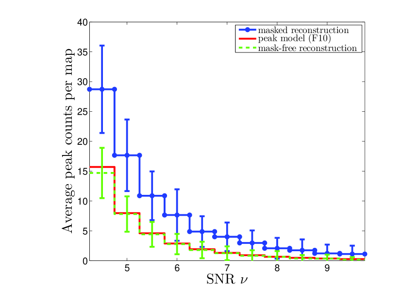
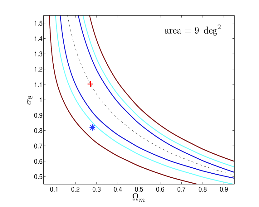
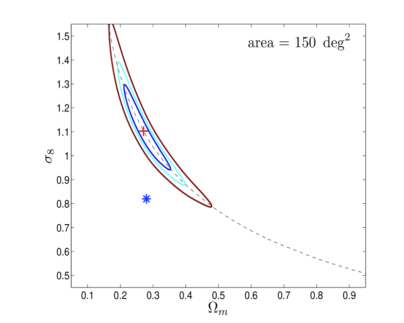
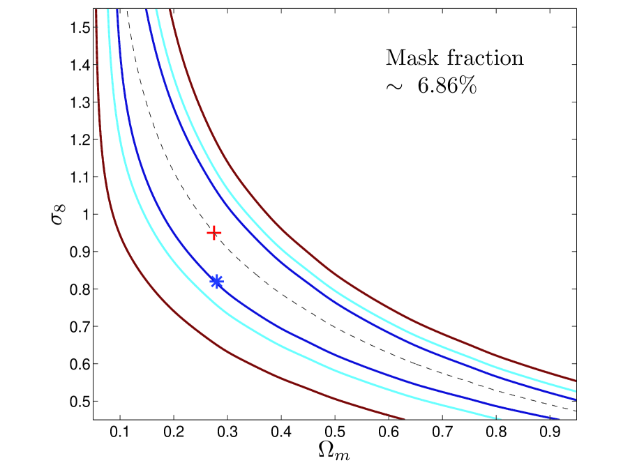
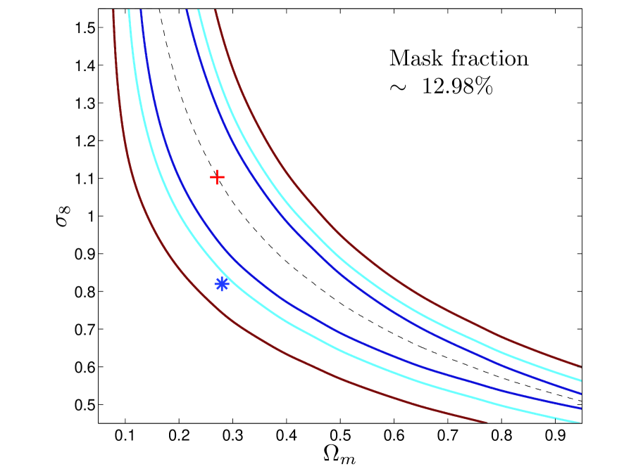
Fig. 11 shows the effects of masks on the peak counts, where the peak counts are calculated by averaging over $128$ maps in each case and $\nu$ is computed with $\sigma_{0}=0.02$ in all cases. The blue, green and red histograms are for peak counts in the case with masks, without masks and the theoretical prediction of F10 with a uniform noise with $\sigma_{0}=0.02$. It is seen clearly that the peak counts considered here are systematically higher due to the presence of masks. We do not expect the results to change qualitatively with different choices of peak binning. Fig. 12 shows the corresponding fitting results with the survey area of $9\hbox{ deg}^{2}$ (left) and $150\hbox{ deg}^{2}$ (right), respectively. The fittings are done with the ‘observed data’ being the peak counts for the masked case, and the model of F10 with $\sigma_{0}=0.02$ uniformly. The covariance matrix is calculated from the $128$ reconstructed maps with masks. The meanings of the lines and symbols are similar to those of Fig. 7. Clearly, the enhanced peak counts due to the occurrence of masks lead to a large bias in cosmological parameter fitting. Even for a survey of $9\hbox{ deg}^{2}$, the true cosmological parameter values (blue symbols) lie outside the $2\sigma$ contour around the best fit (red symbol). This demonstrates the significance of the mask effects, which must be taken into account carefully in cosmological parameter constraints with weak lensing peak counts. For the results with the survey area of $150\hbox{ deg}^{2}$ (similar to the survey area of CFHTLenS (Erben et al., 2013)), we take a simple approach to rescale the covariance matrix calculated from $128$ masked convergence maps to that of the larger survey area assuming a Poisson scaling relation to the survey area $S$ as $1/S$ (Kratochvil et al., 2010). This may underestimate the covariance matrix by a factor of $\sim 1.5$ given the existence of long-range correlations of the true peaks (Kratochvil et al., 2010).

The above results are shown for the average masked area fraction of $\sim 13\%$ with $N_{mask}=280$ in $9\hbox{ deg}^{2}$. We also analyze how the effects depend on the masked fraction. We consider three cases with the number of masks $N_{mask}=140,280$ and $420$ in $9\hbox{ deg}^{2}$ and the corresponding masked fraction of $\sim 7\%$, $\sim 13\%$ and $\sim 19\%$, respectively. The peak statistics are listed in Table 2. The mask effects are clearly stronger for larger masked fraction. The fraction of peaks with $\nu>3$ is about $7\%$ in the case without masks. This fraction increases to $\sim 9\%$, $\sim 11\%$ and $\sim 13\%$ for $N_{mask}=140,280$ and $420$, respectively. More than $90\%$ and $70\%$ of Type I and Type II affected peaks, respectively, are within the regions around masks with a size of twice the mask radius. The results are further visually illustrated in Fig. 13 with all the symbols the same as those shown in left panel of Fig. 10. The corresponding fitting results for the survey area of $9\hbox{ deg}^{2}$ are shown in Fig. 14. We see that with the increase of the masked fraction, the effects become larger. For the masked fraction of $\sim 19\%$, the bias for $(\Omega_{m},\sigma_{8})$ is already larger than $3\sigma$ for a $9\hbox{ deg}^{2}$ survey.

5.2. Mask effects correction

We have demonstrated in §5.1 that the mask effects on weak lensing peak counts are significant. The subsequent cosmological parameter constraints are largely biased if they are not taken into account properly. We therefore need to explore ways to control the mask effects on cosmological applications with weak lensing peak accounts.

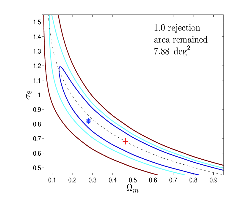
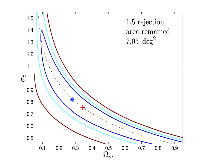
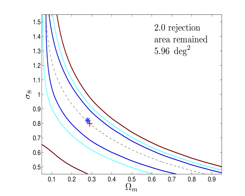
From Table 2 and Fig. 10, we see that the strongly affected peaks are mostly clustered around masks. Thus the first method we use to suppress the mask effects is to exclude the severely affected regions around masks when preforming the peak counting. It is expected that the bias on cosmological parameters can be considerably removed but inevitably at the expense of losing effective survey areas and therefore enlarging the statistical error contours. We name this method as the rejection method. We consider three cases with the rejection regions of $1$, $1.5$ and $2$ times of the mask size around each mask. We pay attention to the mask overlaps. Fig. 15 shows the results, where the model of F10 with a uniform noise of $\sigma_{0}=0.02$ is used in the fitting. The upper left panel shows the result without any rejections, which is the same as the left panel of Fig. 12. The upper right, lower left and lower right panels show the fitting results for the three considered rejections, from the smallest to the largest rejections, respectively. Note that in each case, the covariance matrix used in the fitting is recalculated with the peak counts from the $128$ maps with the corresponding rejections. It is seen that while it is reduced significantly, the bias is still apparent with the rejection of only the masked areas in peak counting (upper right panel). By rejecting regions of $1.5$ times of the mask size around masks, the bias is suppressed to an insignificant level noting the degeneracy direction between the two parameters (lower left panel). To increase the rejection areas further leads to a mild improvement of the fitting result (lower right panel). On the other hand, we see that with the increase of the rejection areas, the confidence contours become larger as expected. We thus conclude that rejecting regions of $1.5\sim 2$ times of mask size around masks is an optimal choice for controlling the bias in cosmological parameter constraints without loosing statistics significantly.

Figure 13.— The illustration of the dependence of the mask effects on the masked fraction. From left to right, the masked area fraction is $\sim 7\%$, $\sim 13\%$, and $\sim 19\%$ ($N_{mask}=140,280$, and $420$ in $9\hbox{ deg}^{2}$), respectively. The meanings of the symbols are the same as those in the left panel of Fig. 10.

Table 2Mask effects on peak statistics with different mask fractions.

$f_{mask}$	$N_{mask}$	$f_{nocorr}$	$f_{offset}$	$f_{\nu\,>3}$	$f_{m,\nu\,>3}$	$f_{LPin}$	$f_{NCin}$	$f_{LIinALL}$
$\sim\,7\%$	$140$	$6.29\%$	$24.05\%$	$6.67\%$	$8.53\%$	$92.67\%$	$72.26\%$	$40.54\%$
$\sim\,13\%$	$280$	$10.97\%$	$40.03\%$	$6.67\%$	$10.93\%$	$93.59\%$	$77.83\%$	$44.13\%$
$\sim\,19\%$	$420$	$15.00\%$	$52.11\%$	$6.67\%$	$12.53\%$	$94.01\%$	$82.24\%$	$47.45\%$

Figure 14.— The corresponding results of cosmological constraints for different masked fractions shown in Fig. 13.

Figure 15.— Results after rejection of regions around masks. The upper left panel is the same as the left panel of Fig. 12, showing the fitting result without any rejections. The upper right panel shows the fitting results with the rejected regions the same as the masked regions. The lower left and right panels are the results for rejections of regions with $1.5$ and $2$ times of mask size, respectively. Here the number of masks is $N_{peak}=280$ in $9\hbox{ deg}^{2}$ and the corresponding masked area fraction is $13\%$.

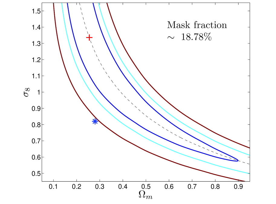
We also explore ways to improve our theoretical modeling to take into account the mask effects properly. From Fig. 10, we see that the significantly affected peaks are closely associated with masked regions, especially those of large masks. Therefore for theoretical modeling, we need to treat these masked regions separately from the rest part of the survey area. For our peak abundance analyses, the presence of masks mainly affects the number of galaxies that are usable in obtaining the smoothed ellipticity field $\langle\boldsymbol{\epsilon}\rangle$ around the masked regions. This in turn leads to non-uniform noises in the convergence field reconstructed from $\langle\boldsymbol{\epsilon}\rangle$ with higher noises near masks than that for the area away from them. These higher noises affect the peak counts in regions around masks in two ways. One is that the systematic peak height shift for true peaks is larger in these regions (F10). The other is the enhancement of the number of noise peaks given their peak heights measured in signal-to-noise ratio with $\sigma_{0}$ still taken to be $0.02$, the value in the mask-free case. The latter can be understood by noting that for different two-dimensional Gaussian random fields, their peak number density distributions are the same if the peak heights in each field are measured in the signal-to-noise ratio defined with the noise level $\sigma_{0}$ of the field itself (e.g., van Waerbeke, 2000). Thus if we use a fixed $\sigma_{0}$ to define the signal-to-noise ratio for peaks in different Gaussian random fields, the peak number distribution would be different for different Gaussian random field. Here due to the presence of masks, the true noise levels around the masks are higher. When counting peaks, however, we use the fixed value $\sigma_{0}=0.02$ (corresponding to $n_{g}=30\hbox{ arcmin}^{-2}$) uniformly to define their signal-to-noise ratios. Therefore the number density of peaks with high $\nu=K_{N}/\sigma_{0}\geq 4$ ($\sigma_{0}=0.02$) is higher than that of the mask-free case.

For further quantitative analyses of the non-uniform noise, we calculate the contribution of source galaxies to each grid point in constructing the smoothed field of $\langle\boldsymbol{\epsilon}\rangle$ by

$$R^{e}(\boldsymbol{\theta})=\frac{\sum_{k=1}^{N_{gal}}R_{k}(\boldsymbol{\theta}_{k})W(\boldsymbol{\theta}_{k}-\boldsymbol{\theta})}{\sum_{k=1}^{N_{gal}}W(\boldsymbol{\theta}_{k}-\boldsymbol{\theta})},$$ (39)

where the summation is over all galaxies with $R_{k}=1$ for galaxies outside masks and $R_{k}=0$ for galaxies inside masks. The kernel $W$ is taken to be the Gaussian smoothing function with $\theta_{G}=1\arcmin$ consistently. The effective number density of source galaxies at each grid point is then estimated by $n_{g}^{e}(\boldsymbol{\theta})=R^{e}(\boldsymbol{\theta})n_{g}$, where $n_{g}=30\hbox{ arcmin}^{-2}$ here. We find that $R^{e}$ can be significantly smaller than $1$ in large mask regions.

Considering the fact that the noise cannot be suitably modeled as a Gaussian random field in regions with $R^{e}\ll 1$, we exclude the circular masked regions with the mask radius larger than $3\arcmin$ from our peak counting analyses. We name these regions as Part I regions which on average occupy about $1\deg^{2}$ over the total $9\deg^{2}$ survey area in our studies. For the remaining $\sim 8\deg^{2}$ area, we develop a two-noise-level model to include the non-uniform noise in our theoretical considerations. Specifically, for each of the $128$ reconstructed convergence maps, we first exclude Part I regions. We then divide the remaining area of each map further into two parts, with Part II being the left over spiked mask regions around the excluded circular regions of Part I, and Part III for the rest of the area. We then calculate the effective number density of source galaxies for Part II and Part III separately by averaging $n_{g}^{e}$ over the grid points inside the corresponding regions and over all the $128$ maps. For Part II, we obtain $n_{g}^{eII}\approx 11.4\hbox{ arcmin}^{-2}$, considerably smaller than $n_{g}=30\hbox{ arcmin}^{-2}$. For Part III, $n_{g}^{eIII}\approx 28.4\hbox{ arcmin}^{-2}$ which is close to $30\hbox{ arcmin}^{-2}$ as expected.

Figure 16.— Left: Average peak counts. The blue histograms with error bars are for the results from masked reconstructed maps excluding Part I regions. The red histograms are calculated with our two-noise-level model. Right: The corresponding cosmological constraints. Here $N_{peak}=280$.

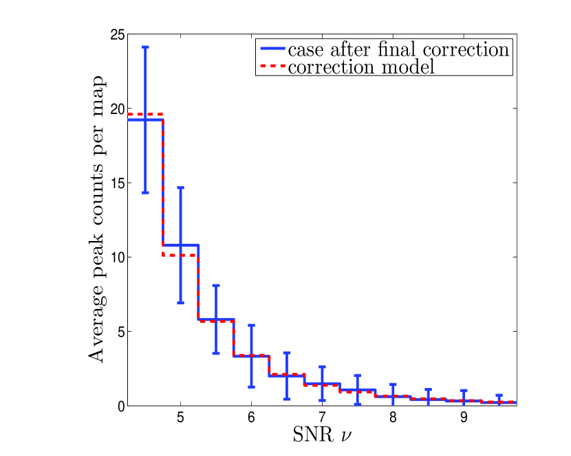
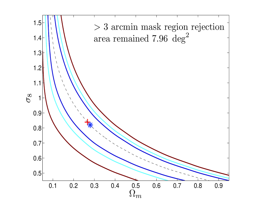
With $n_{g}^{eII}$ and $n_{g}^{eIII}$, we calculate the expected number density of peaks with the model of F10 separately for Part II and Part III regions. We then rescale the signal-to-noise ratios of the peaks in the two regions by a uniform noise level $\sigma_{0}=0.02$, the value used in counting peaks from simulated maps, to obtain the rescaled number density of peaks $n_{peak}^{II}$ and $n_{peak}^{III}$, respectively. The average areas of the two regions $S^{II}$ and $S^{III}$ over a map are computed from the $128$ reconstructed maps with masks by $S^{II}=(\sum_{i=1}^{128}S^{II}_{i})/128$ where $S^{II}_{i}$ is the area of Part II in map $i$, and similarly for $S^{III}$. The theoretical predictions for the total number of peaks in each S/N bin (with $\sigma_{0}=0.02$) over a map is then calculated by $n_{peak}^{II}S^{II}+n_{peak}^{III}S^{III}$. These theoretical predictions are then compared with the corresponding mean ‘observed’ numbers of peaks obtained by averaging over the $128$ counted numbers of peaks directly from the reconstructed convergence maps with masks after the exclusion of Part I regions. We note that in this treatment, the effective usable area over a map $S^{II}+S^{III}\approx 8\deg^{2}$, in comparison with $\sim 7\deg^{2}$ and $\sim 6\deg^{2}$ for the pure rejection analyses with the rejection areas of $1.5$ times and $2$ times of the mask size around each mask, respectively (see Fig. 15.)

The results are shown in Fig. 16 with the left panel for the peak counts and the right panel for the fitting results from our two-noise-level model. The blue, and red histograms in the left panel correspond to the results from the reconstructed convergence maps with masks excluding Part I regions, and the theoretical prediction from the two-noise-level model, respectively, where the signal-to-noise ratio $\nu$ in the horizontal axis is defined with $\sigma_{0}=0.02$. It is seen that the theoretical predictions agree well with the simulation results. The right panel presents the corresponding constraint for $(\Omega_{m},\sigma_{8})$. Comparing to the result shown in the left panel of Fig. 12, we see that our treatment here works well and improves the fitting dramatically with a much reduced bias.

6. Summary and discussion

In this paper, we analyze the mask effects on weak lensing convergence peak statistics and the consequent cosmological parameter constraints from weak lensing peak counts. We run large sets of ray-tracing simulations to generate base convergence and shear maps assuming the source redshift $z_{s}=1$. By randomly populating source galaxies with intrinsic ellipticities, we perform convergence reconstruction from $\langle\boldsymbol{\epsilon}\rangle$, the smoothed field of the ‘observed’ ellipticities of source galaxies, for cases without and with masks, respectively. The mask size distribution from Shan et al. (2012) is adopted. We then investigate in detail the mask effects on weak-lensing peak counts by comparing the results from the two cases. Their influences on cosmological parameter constraints derived from peak abundances are further studied using the peak model of F10 including the noise effects. The validity of this model in terms of the cosmological dependence of peak abundances are tested with simulations.

Our main results are summarized as follows.

(1) The occurrence of masked regions reduces the number of usable source galaxies and therefore increases the noise in the regions around masks. This in turn leads to systematic increases of the number of high peaks and consequently a significant bias in cosmological parameters constrained from weak lensing peak counts. The larger the masked area fraction is, the larger the effects are.

(2) We find that the strongly affected region around a mask is about $1.5\sim 2$ times of the mask size. Excluding such regions in peak counting can eliminate largely the mask effects and therefore reduce the bias in cosmological parameter constraints significantly

(3) We develop a two-noise-level model that treats the mask affected regions separately. This model can account for the mask effects on weak lensing peak counts very well except for very large masked regions with radius larger than $3\arcmin$ where the noise cannot be suitably modeled as a Gaussian random field. These very large masks need to be excluded in peak analyses. Then the constraints on cosmological parameters based on the two-noise-level model improve dramatically comparing to the large bias from the model with a uniform noise.

In our analyses, we apply the Kaiser-Squires method for the nonlinear convergence reconstruction with a Gaussian filter. For the maximum-likelihood reconstruction method (Bartelmann et al., 1996), we expect that the mask effects on the reconstructed convergence field and the peak counts are qualitatively similar to the results shown in this paper although quantitative studies are still needed. For other methods, such as the multi-scale entropy restoration filtering, namely MRLens (Starck et al., 2006), the mask effects can be different and detailed analyses should be carried out when a specific reconstruction method is used. It is also noted that while qualitatively similar mask effects on peak abundances are expected, different filter functions used in the convergence reconstruction and different peak binning methods used in the analyses can lead to quantitatively different results.

The model of F10 and the improved two-noise-level model for the mask effects contain only the noise effects without including the projection effects of large-scale structures and the complex mass distribution of dark matter halos. While the noise from intrinsic ellipticities is the dominant source of errors in weak-lensing peak analyses and our results show that the model(s) can indeed give rise to very good descriptions of the peak counts, future large surveys aiming at high precision cosmological studies need more accurate modeling of the peak counts theoretically. We will explore further improvements of the model carefully in our future studies.

7. Acknowledgement

We thank the referees for the comments that help to improve the paper significantly. We are grateful for the discussions with David Wittman that stimulate the studies on the mask effects, and with Huanyuan Shan and Ran Li. We also sincerely thank the support of Hu Zhan from National Astronomical Observatories, Chinese Academy of Sciences. This research is supported in part by the NSFC of China under grants 11333001, 11173001 and 11033005, and the 973 program No. 2007CB815401.

References

- Abate et al. (2012) Abate, A., Aldering, G., Allen, S. W., et al., 2012, arXiv:1211.0310
- Albrecht et al. (2006) Albrecht, A., et al., 2006, arXiv:astro-ph/0609591
- Amara & Refregier (2008) Amara, A., & Refregier, A., 2008, MNRAS, 391, 228
- Amendola et al. (2012) Amendola, L., Appleby, S., Bacon, D., et al., 2012, arXiv:1206.1225
- Bardeen et al. (1986) Bardeen, J. M., Bond, J. R., Kaiser, N., & Szalay, A. S. 1986, ApJ, 304, 15
- Bartelmann (1995) Bartelmann, M., 1995, A&A, 303, 643
- Bartelmann et al. (1996) Bartelmann, M., Narayan, R., Seitz, S., & Schneider, P., 1996, ApJ, 464, L115
- Bartelmann & Schneider (2001) Bartelmann M., Schneider P., 2001, Phys. Rep., 340, 291
- Bhattacharya et al. (2013) Bhattacharya S., Habib S., Heitmann K., & Vikhlinin A., 2013, ApJ, 766, 32
- Bond & Efstathiou (1987) Bond, J. R., & Efstathiou, G., 1987, MNRAS, 226, 655
- Bridle & King (2007) Bridle, S., & King, L. J., 2007, NewJ.Phys., 9, 444
- Bryan & Norman (1998) Bryan, G. L., & Norman, M. L., 1998, ApJ, 495, 80
- Bullock et al. (2001) Bullock, J. S., et al., 2001, MNRAS, 321, 559
- Carroll et al. (1992) Carroll, S. M., Press, W. H., & Turner, E. L., 1992, ARA&A, 30, 499
- Courtin et al. (2011) Courtin, J., Rasera, Y., Alimi, J. M., Corasaniti, P. S., Boucher, V., & Fuzfa, A., 2011, MNRAS, 410, 1911
- Crocce et al. (2006) Crocce, M., Pueblas, S., & Scoccimarro, R., 2006, MNRAS, 373, 369
- Dietrich & Hartlap (2010) Dietrich, J. P., & Hartlap, J., 2010, MNRAS, 402, 1049
- Eisenstein & Hu (1998) Eisenstein, D. J., & Hu, W., 1998, ApJ, 496, 605
- Eisenstein & Hu (1999) Eisenstein, D. J., & Hu, W., 1999, ApJ, 511, 5
- Erben et al. (2013) Erben, T., Hildebrandt, H., Miller, L., et al., 2013, MNRAS, 433, 2545
- Fan (2007) Fan, Z. H., 2007, ApJ, 669, 10
- Fan et al. (2010) Fan, Z. H., Shan, H. Y., & Liu, J. Y., 2010, ApJ, 719, 1408
- Gavazzi & Soucail (2007) Gavazzi, R., & Soucail, G., 2007, A&A, 464, 399
- Hamana et al. (2004) Hamana, T., Takada, M., & Yoshida, N., 2004, MNRAS, 350, 893
- Hamana et al. (2012) Hamana, T., Oguri, M., Shirasaki, M., & Sato, M., 2012, MNRAS, 425, 2287
- Hartlap, Simon & Schneider (2007) Hartlap, J., Simon, P., & Schneider, P., 2007, A&A, 464, 399
- Hennawi & Spergel (2005) Hennawi, J, F., & Spergel, D. N., 2005, ApJ, 624, 59
- Henry (2000) Henry, J. P., 2000, ApJ, 534, 565
- Heymans et al. (2012) Heymans, C., van Waerbeke, L., Miller, L., et al., 2012, MNRAS, 427, 146
- Hikage et al. (2011) Hikage, C., Takada, M., Hamana, T., & Spergel, D., 2011, MNRAS, 412, 65
- Hilbert et al. (2009) Hilbert, S., Hartlap, J., White, S. D. M., & Schneider, P. 2009, A&A, 499, 31
- Hilbert et al. (2012) Hilbert, S., Marian, L., Smith, R. E., & Desjacques, V., 2012, MNRAS, 426, 287
- Hinshaw et al. (2013) Hinshaw, G., Larson, D., Komatsu, E., et al., 2013, ApJS, 208, 19
- Hoekstra & Jain (2008) Hoekstra, H., & Jain, B., 2008, Annual Review of Nuclear and Particle Science, 58, 99
- Hoekstra, Yee & Gladders (2002) Hoekstra, H., Yee, H. K. C., Gladders, M. D., 2002, New Astro. Rev., 46, 767
- Kaiser (1998) Kaiser, N., 1998, ApJ, 498, 26
- Kaiser & Squires (1993) Kaiser, N. & Squires, G., 1993, ApJ, 404, 441
- Kilbinger et al. (2012) Kilbinger, M., Fu, L. P., Heymans, C., et al., 2012, MNRAS, 430, 2200
- Komatsu et al. (2011) Komatsu, E., Smith, K. M., Dunkley, J., et al., 2011, ApJS, 192, 18
- Kratochvil et al. (2010) Kratochvil, J. M., Haiman, Z., & May, M., 2010, Phys. Rev. D, 81, 043519
- Lewis et al. (2000) Lewis, A., Challinor, A., & Lasenby, A. 2000, ApJ, 538, 473
- Limber (1954) Limber, D. N., 1954, ApJ, 119, 655
- Ma et al. (2006) Ma, Z., Hu, W., & Huterer, D., 2006, ApJ, 636, 21
- Marian et al. (2009) Marian, L., Smith, R. E., & Bernstern, G. M., 2009, ApJ, 698, L33
- Marian et al. (2012) Marian, L., Smith, R. E., Hilbert, S., Schneider, P., 2012, MNRAS, 423, 1711
- Marian et al. (2013) Marian, L., Smith, R. E., Hilbert, S., Schneider, P., 2013, MNRAS, 432, 1338
- Maturi et al. (2010) Maturi, M., Angrick, C., Pace, F., Bartelmann, M., 2010, A&A, 519, 23
- Munshi et al. (2008) Munshi, D., et al., 2008, Phys. Rep., 462, 67
- Navarro et al. (1996) Navarro, J., Frenk, C., & White, S. D. M., 1996, ApJ, 462, 563
- Navarro et al. (1997) Navarro, J., Frenk, C., & White, S. D. M., 1997, ApJ, 490, 493
- Sato et al. (2009) Sato, M., Hamana, T., Takahashi, R., Takada, M., Yoshida, N., Matsubara, T., & Sugiyama, N., 2009, ApJ, 701, 945
- Schirmer et al. (2007) Schirmer, M., Erben, T., Hetterscheidt, M., & Schneider, P., 2007, A&A, 462, 875
- Schneider (1996) Schneider, P., 1996, MNRAS, 283, 837
- Schneider & Seitz (1995) Schneider, P. & Seitz, C., 1995, A&A, 294, 411
- Schneider et al. (1998) Schneider, P., van Waerbeke, L., Jain, B., & Kruse, G., 1998, MNRAS, 296, 873
- Seitz & Schneider (1997) Seitz, C. & Schneider, P., 1997, A&A, 318, 687
- Shan et al. (2012) Shan, H. Y., , Kneib, J. P., Tao, C., et al., 2012, ApJ, 748, 56
- Sheth & Tormen (1999) Sheth, R. K., & Tormen, G., 1999, MNRAS, 308, 119
- Shirasaki et al. (2013) Shirasaki, M., Yoshida, N., & Hamana, T., 2013, ApJ, 774, 111
- Simpson et al. (2013) Simpson, F., Heymans, C., Parkinson, D., et al., 2013, MNRAS, 429, 2249
- Spergel et al. (2003) Spergel, D. N., et al., 2003, ApJS, 148, 175
- Springel (2005) Springel, V., 2005, MNRAS, 364, 1105
- Starck et al. (2006) Starck, J. L., Pires, S., & Refregier, A., 2006, A&A, 451, 1139
- Sun et al. (2009) Sun, L., Fan, Z. H., Tao, C., Kneib, J.-P., Jouvel, S., & Tilquin, A., 2009, ApJ, 699, 958
- Takada & Jain (2003) Takada, M., & Jain, B., 2003, MNRAS, 340, 580
- Takahashi et al. (2012) Takahashi, R., Sato, M., Nishimichi, T., Taruya, A., & Oguri, M., 2012, ApJ, 761, 152
- Tang & Fan (2005) Tang, J. Y., & Fan, Z. H., 2005, ApJ, 635, 60
- van Waerbeke (2000) van Waerbeke, L., 2000, MNRAS, 313, 524
- van Waerbeke et al. (2013) van Waerbeke, L., Benjamin, J., Erben, T. et al., 2013, MNRAS, 433, 3373
- van Waerbeke, Mellier & Hoekstra (2005) van Waerbeke, L., Mellier, Y., & Hoekstra, H., 2005, A&A, 429, 75
- von der Linden et al. (2006) von der Linden, A., Erben, T., Schneider, P., & Castander, F. J., 2006, A&A, 454, 37
- Wang et al. (2009) Wang, S., Haiman, Z., & May, M., 2009, ApJ, 691, 547
- White et al. (2002) White, M., van Waerbeke, L., & Mackey, J., 2002, ApJ, 575, 640
- White & Vale (2004) White, M., & Vale, C., 2004, Astropart.Phys, 22, 27
- Wittman et al. (2006) Wittman, D., Dell’Antonio, I. P., Hughes, J. P., et al., 2006, ApJ, 643, 128
- Yang et al. (2011) Yang, X. J., Kratochvil, J. M., Wang, S., Lim, E. A., Haiman, Z., May, M., 2011, Phys. Rev. D., 84, 043529
- Yang et al. (2013) Yang, X. J., Kratochvil, J. M., Huffenberger, K., Haiman, Z., & May, M., 2013, Phys. Rev. D., 87, 023511