Zero Temperature Phase Diagram of the Classical Kane-Mele-Heisenberg Model

Abstract

The classical phase diagram of the Kane-Mele-Heisenberg model is obtained by three complementary methods: Luttinger-Tisza, variational minimization, and the iterative minimization method. Six distinct phases were obtained in the space of the couplings. Three phases are commensurate with long-range ordering, planar Néel states in horizontal plane (phase.I), planar states in the plane vertical to the horizontal plane (phase.VI) and collinear states normal to the horizontal plane (phase.II). However the other three, are infinitely degenerate due to the frustrating competition between the couplings, and characterized by a manifold of incommensurate wave-vectors. These phases are, planar helical states in horizontal plane (phase.III), planar helical states in a vertical plane (phase.IV) and non-coplanar states (phase.V). Employing the linear spin-wave analysis, it is found that the quantum fluctuations select a set of symmetrically equivalent states in phase.III, through the quantum order-by-disorder mechanism. Based on some heuristic arguments is argued that the same scenario may also occur in the other two frustrated phases VI and V.

I Introduction

The search for the Quantum spin liquid (QSL), a state preserving all the symmetries of a system at zero temperature, on the two dimensional systems with honeycomb geometry has been encouraged after the quantum Monte Carlo study of Hubbard model on the honeycomb lattice meng . This work identified a gapped QSL state, between the Mott-insulator and semi-metal phases, in a narrow interval of moderate on-site Coulomb interactions. Although, the existence of such a QSL phase was debated in more recent works debate1 ; debate2 ; debate3 , a bunch of researches was prompted to study the effective spin models on the honeycomb lattice, arising at the strong coupling limit of the Hubbard model, among which the $J_{1}-J_{2}$ model (with positive nearest,$J_{1}$, and next nearest neighbor, $J_{2}$, exchange interactions) is the minimal spin Hamiltonian kawamura ; aron2010 ; sd2 ; mosadeq ; pvb2 ; pvb3 ; pvb4 ; pvb5 ; pvb6 ; pvb7 ; qsl1 ; qsl2 ; qsl3 ; qsl4 ; qsl5 ; qsl6 ; qsl7 ; eps ; ring1 ; ring2 . Being bipartite, the Néel ordered ground state is stable for small values of $J_{2}$ on the honeycomb lattice. However, it has been shown that for $S=1/2$, the staggered magnetization is reduced by about fifty percent with respect to the classical value, because of the enhanced quantum fluctuations due to the small coordination number of the latticen1 ; n2 ; n4 . The next nearest neighbor interaction, $J_{2}$, tends to destabilize the Néel ordering and destroys it at a critical value $J_{2}/J_{1}\sim 0.2$. Various proposals have been put forward for the nature of the disordered phase, such as staggered dimerized aron2010 ; sd2 (a valence bond crystal state breaking the rotational symmetry of the lattice ), plaquette valence bond crystal mosadeq ; pvb2 ; pvb3 ; pvb4 ; pvb5 ; pvb6 ; pvb7 (a resonating valence bond state breaking the translational symmetry of the lattice), and quantum spin liquid  qsl1 ; qsl2 ; qsl3 ; qsl4 ; qsl5 ; qsl6 ; qsl7 .

The theoretical and experimental achievements in the field of topological insulators (TI) TI1 ; TI2 , attracts many attentions for exploring the effect of electron-electron interaction in the systems with strong spin-orbit coupling, where the topological features arises TI-int . One of the earliest model in this context, introduced by Kane and Mele (KM), which is a tight-binding model of non-interacting electrons on a honeycomb lattice subjected to a spin-orbit term Kane2005 . Electron-electron interaction can be introduced to the KM model by adding an on-site repulsive Hubbard term to this model, resulting in a Hamiltonian, so-called the Kane-Mele-Hubbard model. Analytic as well as the numeric study of this model, suggest a QSL phase at the moderate Hubbard interaction, between the topological band insulator (TBI) and Mott insulator phases Rachel2010 ; kmh1 ; kmh2 ; kmh3 ; kmh4 ; kmh5 ; kmh6 ; kmh7 ; kmh8 ; kmh9 . The strong coupling limit ($U\gg t$) of the model can be described, effectively, by a XXZ spin Hamiltonian namely, the Kane-Mele-Heisenberg (KMH) model Rachel2010 ; vaezi . Recently, Vaezi et al vaezi , using the Schwinger-boson and Schwinger-fermion methods, proposed a chiral spin liquid state for this model, in a narrow region of the phase diagram, the rest of which is divided into the Néel and incommensurate Néel ordered phases.

A promising guideline of finding the possibility of the spin liquid state for a spin Hamiltonian, is exploring of its classical phase diagram (the large-$S$ limit), at zero temperature. The regions in the phase diagram where the classical ground state is highly degenerate, due to the competition between the couplings, are likely to be QSL in the quantum limit. The classical phase diagram of the Anti-ferromagnetic Heisenberg model on the honeycomb lattice, up to third neighbor interaction, has been extensively studied earlier Rastelli ; Fouet , and various ordered phases as well as a region of magnetically disordered phase has been obtained.

The absence of such an analysis for the KMH model was our motivation for this work. We use Luttinger-Tisza, Variational and Iterative minimization methods, each being complementary of the other, to obtain the classical phase diagram of the KMH model. The rest of paper is organized as the following. In Sec.II, the KMH model is introduced, Sec.III is devoted to the extraction of the classical phase diagram by the three mentioned methods. Using linear spin wave theory, we calculate the quantum correction in Sec.IV, and investigate the stability of the classical phase as well as the possibility of quantum order-by-disorder in the classically degenerate regions. finally, we summarize the results in Sec.V.

II Kane-Mele-Heisenberg Model

Kane and Mele Kane2005 proposed a model for describing the quantum spin Hall (QSH) effect in graphene, by adding a mass term to the nearest neighbor tight-binding Hamiltonian. The model is defined by the following Hamiltonian

$$H_{\textbf{KM}}=-t\sum_{\langle ij\rangle,\sigma}c_{i\alpha}^{\dagger}c_{j\alpha}+i\lambda\sum_{\langle\!\langle i,j\rangle\!\rangle,\alpha\beta}\nu_{ij}\sigma_{\alpha\beta}^{z}c_{i\alpha}^{\dagger}c_{j\beta},$$ (1)

in which the first term represents the hopping between the nearest neighbors of a honeycomb lattice, and the second term , with $\nu_{ij}=\pm 1$ being an anti-symmetric tensor, denotes the next nearest neighbor spin-orbit hopping integral which gives rise to the topological features, such as the edge state modes.

Adding electron-electron interaction to the Kane-Mele Hamiltonian, Eq. (1), by an on-site repulsive Hubbard term

$$H_{U}=\sum_{i}Un_{i\uparrow}n_{i\downarrow},$$ (2)

gives the Kane-Mele-Hubbard model. In the limit where the on-site coulomb repulsion $U$ is much larger than the hopping integrals $t$ and $\lambda$, the charge fluctuations are suppressed, and one can project the half-filled Hamiltonian to the lowest Hubbard sub-band for which the condition of the single-occupied site is fulfilled. This procedure can be done perturbatively in terms of the ratios $t/U$ and $\lambda/U$. To the fourth order, we find a spin Hamiltonian called the Kane-Mele-Heisenberg (KMH) model as followingRachel2010 ; vaezi

$$\begin{split}H_{\textbf{KMH}}\!\!&=\!\!J_{1}\sum_{\langle i,j\rangle}{\bf S}_{i}\cdot{\bf S}_{j}+J_{2}\sum_{\langle\!\langle i,j\rangle\!\rangle}{\bf S}_{i}\cdot{\bf S}_{j}\\ &+g_{2}\sum_{\langle\!\langle i,j\rangle\!\rangle}(-S_{i}^{x}~{}S_{j}^{x}-S_{i}^{y}~{}S_{j}^{y}+S_{i}^{z}~{}S_{j}^{z}),\end{split}$$ (3)

in which $J_{1}=4t^{2}/U-16{t^{4}}/U^{3}$, $J_{2}=4{t^{4}}/U^{3}$ and $g_{2}=4{\lambda^{2}}/U$ are the first and second neighbor exchange couplings and ${\bf S}_{i}$ represents an $S=1/2$ spin residing in site $i$. We are interested in classical phase diagram of this model, hence in the large $S$ limit , we consider the spins as unit vectors. In the next section we use three methods to find the classical phase diagram at the zero temperature.

III Classical phase diagram of KMH model

III.1 Luttinger-Tisza(LT) Method

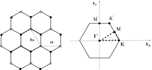
Figure 1: Left: geometry of the real space honeycomb lattice. Primitive vectors are denoted by ${\bf a}$ and ${\bf b}$, and the open and filled circles denote the two triangular sub-lattice points. Right:The first Brillouin zone of the honeycomb lattice.

The LT method LT ; Kaplan1960 ; Kaplan2006 is a way of finding the ground state of a classical quadratic Hamiltonian. By Fourier transformation of the spins and the couplings, one can find a matrix representation for a quadratic spin Hamiltonian in the Fourier space. The lowest eigenvalues and eigenvectors of this matrix give the ground state energy and the corresponding spin structure factor, respectively.

Honeycomb lattice is composed of the two triangular sub-lattices (Fig. 1), therefore the Fourier transformations of the spins for each sub-lattice become:

$$\begin{split}\textbf{S}^{1}({\bf r}_{i})=\frac{1}{\sqrt{N/2}}\sum_{\bf q}\textbf{S}^{1}_{\bf q}e^{-i\textbf{q}\cdot\textbf{r}_{i}},\\ \textbf{S}^{2}({\bf r}_{i})=\frac{1}{\sqrt{N/2}}\sum_{\bf q}\textbf{S}^{2}_{\bf q}e^{-i\textbf{q}\cdot\textbf{r}_{i}},\end{split}$$ (4)

where $\textbf{r}_{i}$ denote the translational vectors of the triangular Bravais lattice and $N/2$ is the number of primitive cells, and the superscripts denote the sub-lattices. Substituting the above transformations into the classical KMH Hamiltonian, Eq.(3), one gets the following form for the Hamiltonian in terms of the Fourier components:

$$H^{\rm cl}_{\textbf{KMH}}=\sum_{{{\bf{q}}}}{\bf S}^{t}_{-{{\bf{q}}}}\cdot{\bf M}_{{{\bf{q}}}}\cdot{\bf S}_{{{\bf{q}}}},$$ (5)

in which ${\bf S}^{t}_{-{{\bf{q}}}}=\begin{pmatrix}S_{-{{{\bf{q}}}},x}^{1}\ S_{-{{\bf{q}}},y}^{1}\ S_{-{{\bf{q}}},z}^{1}\ S_{-{{\bf{q}}},x}^{2}\ S_{-{{\bf{q}}},y}^{2}\ S_{-{{\bf{q}}},z}^{2}\end{pmatrix}$, and the matrix ${\bf M}_{{{\bf{q}}}}$ is defined as

$${\bf M}_{q}=\begin{pmatrix}A_{{\bf{q}}}&0&0&C_{{\bf{q}}}&0&0\\ 0&A_{{\bf{q}}}&0&0&C_{{\bf{q}}}&0\\ 0&0&B_{{\bf{q}}}&0&0&C_{{\bf{q}}}\\ C^{*}_{{\bf{q}}}&0&0&A_{{\bf{q}}}&0&0\\ 0&C^{*}_{{\bf{q}}}&0&0&A_{{\bf{q}}}&0\\ 0&0&C^{*}_{{\bf{q}}}&0&0&B_{{\bf{q}}}\end{pmatrix}$$ (6)

whose elements are given by

$$A_{{\bf{q}}} = 2(J_{2}\!-\!g_{2})[\cos q_{a}\!+\!\cos q_{b}\!+\!\cos(q_{a}\!+\!q_{b})]$$

$$B_{{\bf{q}}}\! \!=\! \!2(J_{2}\!+\!g_{2})[\cos q_{a}+\cos q_{b}+\cos(q_{a}+q_{b})]$$

$$C_{{\bf{q}}} = J_{1}[1\!+\!\exp({iq_{b}})+\exp({i(q_{a}+q_{b})})].$$ (7)

Here $q_{a}={\bf q}\cdot{\bf a}$ and $q_{b}={\bf q}\cdot{\bf b}$, where ${\bf a}=\hat{\bf x}$ and ${\bf b}=-1/2~{}\hat{\bf x}+{\sqrt{3}}/{2}~{}\hat{\bf y}$ are the primitive translational vectors of the honeycomb lattice displayed in Fig. 1. Writing Eq.(5) in terms of the eigen-modes of ${\bf M}_{{{\bf{q}}}}$, leads us to the following simple quadratic form

$$H^{\rm cl}_{\textbf{KMH}}=\sum_{\mu}\sum_{{{\bf{q}}}}\lambda_{{{\bf{q}}}}^{\mu}|{\tilde{\bf S}}_{{{\bf{q}}}}^{\mu}|^{2}$$ (8)

where $\lambda_{{{\bf{q}}}}^{\mu}$ with $\mu=1,2,3,4,5,6$ are the eigenvalues of ${\bf M}_{{{\bf{q}}}}$, and

$${\tilde{\bf S}}_{{{\bf{q}}}}^{\mu}=w^{\mu}_{{{\bf{q}}}}{\bf S}_{{{\bf{q}}}},$$ (9)

denotes the spin structure factors, with $w^{\mu}_{{{\bf{q}}}}$ being the eigenvectors of ${\bf M}_{{{\bf{q}}}}$ with eigenvalue $\lambda_{{{\bf{q}}}}^{\mu}$.

$${\bf M}_{{{\bf{q}}}}w^{\mu}_{{{\bf{q}}}}=\lambda_{{{\bf{q}}}}^{\mu}w^{\mu}_{{{\bf{q}}}}.$$ (10)

The size of spins being unity at each site, requires the following constraint be satisfied by the Fourier components

$$\sum_{i}|{\bf S}_{i}|^{2}=\sum_{{{\bf{q}}}}|\tilde{\bf S}_{{{\bf{q}}}}|^{2}=N.$$ (11)

If a global minimum $\lambda_{0}$ is found among the eigenvalues, using Eq.(11) the classical energy (Eq.(8)) can be rewritten as

$$H^{\rm cl}_{\textbf{KMH}}=N\lambda_{0}+\sum_{\mu>0}\sum_{{{\bf{q}}}}(\lambda_{{{\bf{q}}}}^{\mu}-\lambda_{0})|{\tilde{\bf S}}_{{{\bf{q}}}}^{\mu}|^{2}.$$ (12)

Since $\lambda_{{{\bf{q}}}}^{\mu}-\lambda_{0}>0$, the ground state energy per primitive cell is equal to $\lambda_{0}$, provided that all the structure factors other than the one corresponding to the minimum eigenvalue vanishes. These conditions enables us to find the spin configuration in the ground state, as well.

For the KMH model, the eigenvalues of $M_{{{\bf{q}}}}$ are given by

$$\lambda_{1,2}=A_{\bf q}-|{C_{\bf q}|},$$

$$\lambda_{3,4}=A_{\bf q}+|{C_{\bf q}|},$$

$$\lambda_{5}=B_{\bf q}-|{C_{\bf q}|},$$

$$\lambda_{6}=B_{\bf q}+|{C_{\bf q}|},$$ (13)

where $A_{\bf q},B_{\bf q}$ and $C_{\bf q}$ are given by Eq.(7). The two-fold degeneracy of the first two eigenvalues reflects the $O_{2}$ symmetry of the ${\bf KMH}$ model in $x-y$ plane.

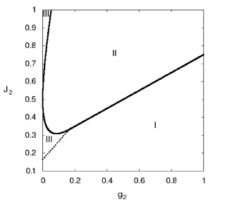
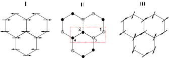
Figure 2: Top: The Luttinger-Tisza phase diagram of the ${\bf{KMH}}$ Hamiltonian in $J_{2}-g_{2}$ space. Solid and dotted curves denote the first-order and secon-order phase boundaries, respectively. Bottom: typical spin configuration in I) Néel-$xy$, II) collinear-$z$ state with the wave-vector ${\bf M}=(\frac{\pi}{a},\frac{\pi}{\sqrt{3}{a}})$ (open and filled circles denote the up and down spin directions, respectively) and III) helical-$xy$ phase.

Setting $J_{1}=1$, we proceed to find the stable phases of the ${\bf KMH}$ model by calculating the minimum eigenvalues of the coupling matrix , for $0<J_{2}<1$ and $0<g_{2}<1$. Fig. 2 represents the phase diagram obtained by LT method, departing the coupling space into the three distinguished regions:

I )In-plane commensurate Néel states (Néel-$xy$))- the minimum eigenvalues indicating this phase are $\lambda_{1,2},$ with the wave-vector $q=(0,0)$ and phase difference $\pi$ between the two spins within each unit-cell. The $O_{3}$ symmetry of Heisenberg Hamiltonian is reduced to $O_{2}$ due to the $g_{2}$ term, laying the spins in the $xy$-plane. The energy per spin in this phase is given by:

$$\epsilon_{I}=3(J_{2}-g_{2})-\frac{3}{2}.$$ (14)

II) Commensurate vertical collinear states ( collinear-$z$): this phase is three-fold degenerate and characterized by alignment of spins along the ${\bf\hat{z}}$ axis, normal to the honeycomb plane. In this phase the eigenvalue $\lambda_{5}$ is minimized by the following three wave-vectors ($M$-points in $1BZ$)

$$q_{x}=\frac{\pi}{a},q_{y}=\pm\frac{\pi}{\sqrt{3}{a}},$$

$$q_{x}=0,q_{y}=\frac{2\pi}{\sqrt{3}{a}},$$ (15)

and the phase difference $\pi$ within each unit-cell. The energy per spin is given by

$$\epsilon_{II}=-(J_{2}+g_{2})-\frac{1}{2}.$$ (16)

The boundary between this phase and the phase.I, is given by

$$J_{2}=\frac{g_{2}}{2}+\frac{1}{4},~{}g_{2}>1/6$$ (17)

which is a first-order transition line.

III) Incommensurate in-plane helical states (helical-$xy$): in this phase, the eigenvalues $\lambda_{1,2}$ become minimum at the incommensurate wave-vector

$$q_{x}=\frac{2}{a}\cos^{-1}\left({\frac{1-2(J_{2}-g_{2})}{4(J_{2}-g_{2})}}\right),q_{y}=0,$$ (18)

and give the energy per spin as

$$\epsilon_{III}=\frac{-1}{8(J_{2}-g_{2})}[1+12{(J_{2}-g_{2})}^{2}].$$ (19)

The line

$$J_{2}=g_{2}+\frac{1}{6},~{}~{}g_{2}<1/6,$$ (20)

is the continuous transition boundary, separating this phase from the phase.I, and the curves

$$J_{2}=3{g_{2}}+\frac{1}{2}-\sqrt{4{g_{2}}^{2}+2g_{2}},~{}~{}g_{2}<1/6,J_{2}<1/2$$

$$J_{2}=3{g_{2}}+\frac{1}{2}+\sqrt{4{g_{2}}^{2}+2g_{2}},~{}~{}g_{2}<1/6,J_{2}>1/2.$$ (21)

determine the borders of phase.III and the phase.II, which are first-order boundaries.

The problem with the LT method is that the ground states derived by this are only consistent with the weak constraint Eq.(11), hence there is no guarantee that the spin configurations with minimum energy satisfy the strong constraint of the unit spin size at each site. Indeed, it gives an upper bound for the classical ground state energy, Moreover the non-coplanar spin configurations can not be found by this method Henley1 ; Henley2 . To search for such states, we parametrize each spin in terms of its wave-vector, polar and azimuthal angles and use variational minimization method to find the ground state.

III.2 Variational minimization Method

In this section we parametrize the spins in such a way that the constraint of the unity of spin size is fulfilled at each lattice site. We start to search for planar states. Consider a planar-$xy$ pattern with wave-vector ${\bf q}$, the spins in this configuration can be parameterized as

$$S^{1}({\bf r}_{i}) = S[\cos({\bf q}.{\bf r}_{i})\hat{\bf x}+\sin({\bf q}.{\bf r}_{i})\hat{\bf y}]$$

$$S^{2}({\bf r}_{i}) = -S[\cos({\bf q}.{\bf r}_{i}+\varphi)\hat{\bf x}+\sin({\bf q}.{\bf r}_{i}+\varphi)\hat{\bf y}],$$ (22)

in which $\varphi+\pi$ denotes the phase difference between the spins in a primitive cell. Substituting Eq.(22) in the ${\bf KMH}$ Hamiltonian (Eq.(3)), we get the following expression for the classical energy per spin

$$\epsilon_{\rm cl} = -\frac{J_{1}S^{2}}{2}[\cos\phi+\cos(\phi-q_{b})+\cos(\phi-q_{a}-q_{b})]$$ (23)

$$+ (J_{2}-g_{2})S^{2}[\cos q_{a}+\cos q_{b}+\cos(q_{a}+q_{b})].$$

Minimization of this energy with respect to $q_{x}$ and $q_{y}$ and $\varphi$, gives $q_{x}=q_{y}=0$ and $\varphi=0$ in the phase.I resulting in the in-plane Néel states.

For the phase.III we get the following relations

$$\cos q^{*}_{a}+\cos q^{*}_{b}+\cos(q^{*}_{a}+q^{*}_{b})=\frac{1}{2}\left[\left(\frac{1}{2(J_{2}-g_{2})}\right)^{2}-3\right],$$

$$\sin\phi^{*}=2{(J_{2}-g_{2})}\left(\sin q^{*}_{b}+\sin(q^{*}_{a}+q^{*}_{b})\right),$$

$$\cos\phi^{*}=2(J_{2}-g_{2})(1+\cos q^{*}_{b}+\cos(q^{*}_{a}+q^{*}_{b})),$$ (24)

meaning the infinitely degenerate set of in-plane helical states, which form a manifold for the ground state. Similar results have already been obtained for $J_{1}-J_{2}$ model ($g_{2}=0$) in Ref. aron2010 . Fig. 3 displays the ground state manifold in the first Brillouin zone. This is in the form a closed countour around $q=(0,0)$ for $1/6<(J_{2}-g_{2})<1/2$, while it encircles the $K$-points for $(J_{2}-g_{2})>1/2$.

Figure 3: The countours of classical ground state. The numbers denote the values of $J_{2}-g_{2}$.

To search for the non-coplanar ground states, one needs to include all the three component of the spins. In the simplest case, the minimum magnetic unit cell of a spin pattern consists of two spins, therefore the spins can be parametrized as the following

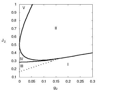
Figure 4: The phase diagram obtained by variational minimization method. This method divides the phase.III, previously obtained by LT method, into three regions. The helical-$xy$ states remain in the region assigned with the phase.III, the incommensurate planar states in a plane vertical to $xy$-plane (phase.IV), and the incommensurate non-coplanar states (phase.V).

$${S^{\alpha}_{i,x}} = S\sin(\theta^{\alpha}_{i})\cos(\phi^{\alpha}_{i}),$$

$${S^{\alpha}_{i,y}} = S\sin(\theta^{\alpha}_{i})\sin(\phi^{\alpha}_{i}),$$

$${S^{\alpha}_{i,z}} = S\cos(\theta^{\alpha}_{i}),$$

in which $\alpha=1,2$, labels the two sub-lattices and

$$\phi^{1}_{i} = {\bf q}\cdot{\bf r}_{i},$$

$$\phi^{2}_{i} = {\bf q}\cdot{\bf r}_{i}+\varphi,$$

$$\theta^{1}_{i} = {\bf q}^{\prime}\cdot{\bf r}_{i}+\gamma,$$

$$\theta^{2}_{i} = {\bf q}^{\prime}\cdot{\bf r}_{i}+\eta.$$ (26)

Substituting the spins by Eq.(LABEL:n-coplan) in the ${\bf KMH}$ Hamiltonian, minimization of the classical energy with respect to the $7$ variables $q_{x},q_{y},{\acute{q}}_{x},{\acute{q}}_{y},\gamma,\eta,\phi$ would give us the ground state energy as well as the corresponding spin configuration. The simulated annealing scheme was used, from the Mathematica optimization package Wolfram , for the numerical minimization of the energy function. The Néel-$xy$ (phase.I) and the collinear-$z$ (phase.II) were easily reproduced by finding $({\bf q}^{\prime}=0,\gamma=\eta=\pi/2)$ for the former and $({\bf q}^{\prime}=M,M^{\prime},M-M^{\prime},\gamma=0,\eta=\pi)$ for the later. The case of interest is the helical-$xy$ (phase.III), for which the energy per spin can be simplified as the following

$$\begin{split}\frac{\epsilon_{cl}}{S^{2}}&=-\frac{J_{1}}{4}\sum_{\delta_{1}}[\cos(\acute{{{\bf{q}}}}.\delta_{1}+\gamma-\eta)(1+\cos({{\bf{q}}}.\delta_{1}-\phi))]\\ &+\frac{(J_{2}-g_{2})}{2}\sum_{\delta_{2}}[\cos({{\bf{q}}}.\delta_{2})\cos(\acute{{{\bf{q}}}}.\delta_{2})]\\ &+\frac{(J_{2}+g_{2})}{2}\sum_{\delta_{2}}\cos(\acute{{{\bf{q}}}}.\delta_{2}).\end{split}$$ (27)

where

$$\delta_{1}={\bf 0},\pm\textbf{b},\pm(\textbf{a+b})$$ (28)

denote the unit cell position vectors of the nearest neighbors of a given lattice point with $-$ and $+$ correspond to $1$ and $2$ sub-lattices, respectively, and

$$\delta_{2}=\pm\textbf{a},\pm\textbf{b},\pm(\textbf{a+b}),$$ (29)

are the position vectors of the second neighbor primitive cells. As shown in Fig. 4, Minimization of this energy tends to the partitioning of the phase.III of the LT phase diagrams into three regions.

i) Incommensurate helical-$xy$ as previously found by LT method and so we call it again phase.III,

ii) Incommensurate planar phase in a plane perpendicular to honeycomb plane (phase.IV). Like the helical-$xy$, this phase is also infinitely degenerate and the minimum energy is achieved by $({\bf q}=0,\varphi=\pi)$ and a set of wave-vectors ${\bf q}^{\prime}$ and phase differences satisfying the following relations

$$\cos q^{\prime*}_{a}+\cos q^{\prime*}_{b}+\cos(q^{\prime*}_{a}+q^{\prime*}_{b})=\frac{1}{2}\left[\left(\frac{1}{2J_{2}}\right)^{2}-3\right],$$

$$\sin(\eta^{*}-\gamma^{*})=2J_{2}\left[\sin q^{\prime*}_{b}+\sin(q^{\prime*}_{a}+q^{\prime*}_{b})\right],$$

$$\cos(\eta^{*}-\gamma^{*})=2J_{2}[1+\cos q^{\prime*}_{b}+\cos(q^{\prime*}_{a}+q^{\prime*}_{b})]$$ (30)

These relations are the same as Eq.(24), except the absence of the coupling $g_{2}$. The reason that $g_{2}$ is omitted from the classical energy in this phase can be explained as the following. Because of the in-plane $O_{2}$ symmetry, one can consider the spins in this state in the $xz$ plane. Thus substituting the $x$ and $z$ components of the spin from Eq.(LABEL:n-coplan) to the ${\bf{KMH}}$ Hamiltonian, one finds that the contribution of the $g_{2}$ term to the energy is as

$$g_{2}\sum_{\ll i,j\gg}2\cos({\bf q}^{\prime}\cdot({{\bf{r}}}_{i}+{{\bf{r}}}_{j})+2\gamma).$$ (31)

Since ${\bf q}^{\prime}$ is not equal to any of the $M$-points in the $1BZ$, then $2{\bf q}^{\prime}\cdot({{\bf{r}}}_{i}+{{\bf{r}}}_{j})\neq 2n\pi$ and so the above summation vanishes. Therefore, all over the phase.IV the energy is independent of $g_{2}$. However, the effect of this term is the breaking of the $O_{3}$ symmetry of the $J_{1}-J_{2}$ Heisenberg Hamiltonian, in such a way that the spins confine in a vertical plane. For small values of $J_{2}$, the $g_{2}$ term cooperates with the $J_{1}$ term to ferro-magnetically align the second neighbors in the $xy$-plane, resulting the in-plane Néel ordering. On the other hand, the term $J_{2}$ tends to align the second neighbor spins anti-parallel, hence increasing $J_{2}$ to above a critical value, the in-plane states become destabilized and system gains energy by lifting the spins out of the honeycomb plane and arrange them in a plane perpendicular to it. It is also found that even for $g_{2}=0$, the co-planar states found to be less energetic than non-coplanar ones, though with a very small energy difference.

iii) the incommensurate non-coplanar phase, called phase.V. This phase is highly degenerate in terms of both the $xy$ and $z$ wave-vectors, however they are not equal in general (${\bf q}\neq{\bf q}^{\prime}$ ). These states are approximately planar normal to $xy$-plane with a small out of plane spin component. The energy landscape in this phase is very flat with a weak dependence on $g_{2}$.

Here, we limit ourselves to the states with two-spins in a unit cell. Extending this method to states with larger magnetic cells is straight forward, however increasing the number of variational parameters makes the finding of the global minimum extremely difficult. Hence to search for such a new state, in the next part we employ a method called iterative minimization.

III.3 Iterative Minimization Method

For extracting the classical phase diagram for ${\bf KMH}$ model we also apply the iterative minimization method Walker ; Henley1 ; Henley2 . In this method we start from an initial state with spins arranged in a random configuration. Then in each step of the iterative process a random spin is selected for adjusting its orientation in order to minimize its energy. The minimization is achieved by aligning the selected spin with the local field produced by its neighbors while keeping its length unity. For the ${\bf KMH}$ model the local field in the position of spin $\textbf{S}_{i}$ is:

$$\begin{split}\textbf{M}_{i}&=J_{1}\sum_{j:\langle i,j\rangle}\textbf{S}_{j}+J_{2}\sum_{j:\langle\!\langle i,j\rangle\!\rangle}\textbf{S}_{j}\\ &+g_{2}\sum_{j:\langle\!\langle i,j\rangle\!\rangle}(-S_{j}^{x}\hat{\textbf{x}}-S_{j}^{y}\hat{\textbf{y}}+S_{j}^{z}\hat{\textbf{z}}),\end{split}$$ (32)

where sums are run over $j$s that are nearest or next nearest neighbors of $i$ site. To minimize energy in each step we adjust spin $\textbf{S}_{i}$ as $\textbf{S}_{i}=-\textbf{M}_{i}/|\textbf{M}_{i}|$. The iterations are continued until the method converges to some (local) energy minimum.

We start with a honeycomb lattice consisting of two triangular sub-lattices of parallelogram shapes with periodic and open boundary conditions and with sizes of $8\times 8$, $16\times 16$, $32\times 32$ and $64\times 64$ sites each in total consisting of $N_{s}$ sites; i.e. $N_{s}$ is 128, 512, 2048 and 8192 respectively. Then we run a large loop, and on each iteration of the loop we pick $N_{s}$ spins for updating.

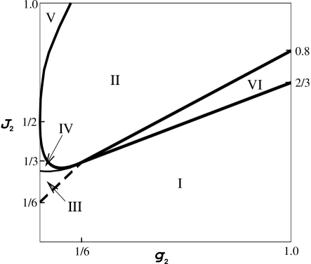
Figure 5: Classical phase diagram for ${\bf KMH}$ model obtained from Iterative minimization method. The newly found phase, called phase.VI, between phase.I and phase.II, is a commensurate-planar state in a vertical plane.

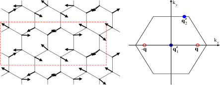
Figure 6: Left: spin configuration in the commensurate coplanar-$xz$ region (phase.VI ). The dashed rectangle shows the magnetic unit cell, consisting of $16$ spins. In this plot the $z$ components have been projected along the $y$-axis in order to show the spin configuration in the $xy$-plane. Right: the wave-vectors corresponding to the Fourier transformation of the spin configuration in phase.VI, in which open and filled circles denote the in plane (${{{\bf{q}}}}^{\prime}$) and normal to plane (${{{\bf{q}}}}$) wave-vectors, respectively.

Once we have obtained a local energy minimum spin configuration, we try to get a sense of the spin configuration by plotting the spin arrangements in real space and looking at their $x$, $y$ or $z$ components. For some cases that the ground state is a commensurate state, the local energy minimum state consists of finite domains similar to the true ground state, separated by domain walls. By restarting the program with a random spin configuration that is close to the proposed true ground state configuration, the program rapidly converges to the true ground state and by comparing its energy we can verify our guess for the ground state. For the regions of the phase diagram that the true ground state is a state commensurate with lattice periodicity, we start from a properly selected random configuration and normally we obtain the true ground state for small size systems with very fast convergence.

We can also calculate the Fourier transforms of the spins to get an idea of the spin configuration. This method is suitable for both commensurate and incommensurate states. After calculating the Fourier transforms of spin components we plot the distribution of the Fourier magnitudes of spin components in the first Brillouin zone. Normally, we observe one or a few peaks in the Brillouin zone, which gives the wave vector components of the state.

The classical phase diagram obtained from this method is shown in Fig. 5. For small values of $J_{2}$ the system shows Néel ordering in $xy$-plane (Phase.I) with zero wave-vector. For $g_{2}>1/6$, increasing the value of $J_{2}$ the system goes to a co-linear $z$ state which has three-fold degeneracy with wave-vector one of $M$-points (phase.II). However, At the border phase.I and phase.II we found a new narrow region with commensurate co-planar spin state in a plane perpendicular to the $xy$- plane (here we call it coplanar-$xz$ or phase.VI). One realization of the spin configurations in this region is shown in Fig. 6. Unlike, the helical states the in-plane and normal to plane spin components have different wave-vectors in reciprocal space. The $z$ spin component has two Fourier components with the wave-vectors ${\bf q}=\pm(\pi,0)$, while the in-plane spin component is a linear combination of two Fourier components with the wave-vectors ${\bf q}^{\prime}_{1}=(0,0)$ and ${\bf q}^{\prime}_{2}=(\frac{\pi}{2},\frac{2\pi}{\sqrt{3}})$ (Fig. 6). On the other hand the phase difference between the $x$-components in each unit cell is $\pi$, while the $z$-components are in the same phase, thus the spin components in this phase can be written as

$$S^{1}_{x}({{{\bf{r}}}})=-S^{2}_{x}({{{\bf{r}}}})=B_{0}+B_{1}\cos({{{\bf{q}}}}^{\prime}\cdot{{{\bf{r}}}}+{\phi}^{\prime})$$

$$S^{1}_{z}({{{\bf{r}}}})=S^{2}_{z}({{{\bf{r}}}})=A\cos({{{\bf{q}}}}\cdot{{{\bf{r}}}+\phi}).$$ (33)

For $g_{2}<1/6$, we observe several coplanar and non-coplanar incommensurate states. Close to $g_{2}=0$ axis we found two degenerate incommensurate state phase regions. Our results reproduce the results of Mulder et al aron2010 for $g_{2}=0$. In the absence of $g_{2}$ for $\frac{1}{6}<J_{2}/J_{1}<\frac{1}{2}$ there is a circular manifold of classically degenerate spiral state wave vectors centered at origin. We found that by turning on $g_{2}$, the spiral state remains stable but it becomes non-coplanar until $g_{2}$ exceeds $J_{2}-\frac{1}{6}$ and the system makes a transition to the coplanar-$xy$ state. By looking more precisely to this region we found that indeed this region is composed from two sub-regions of nearly coplanar-$xy$ and nearly coplanar-$xz$ states. The nearly coplanar-$xz$ state is situated above the nearly coplanar-$xy$ phase for $J_{2}$ greater than around $0.30$. For $J_{2}/J_{1}>\frac{1}{2}$ we found a degenerate spiral state with a closed manifolds of stable wave vectors centered at the corners of the Brillouin zone. Again this state remains stable by turning on $g_{2}$ but it becomes non-planar until the system makes a transition to the collinear-$z$ state. We also found that the manifold of degenerate energy region in the Brillouin zone only depends on $J_{2}$ and is independent of $g_{2}$.

IV Linear Spin Wave Analysis

In this section we use the linear spin-wave (LSW) theory to calculate the zero point quantum corrections to the classical ground state energy. Moreover, This method enables us to investigate the stability of a classical state against the quantum fluctuations, by calculating the excitation spectrum. For a given classical spin configuration, first it is convenient to apply an appropriate local rotation on each site, in order to turn the local $z$-axis along the spin direction on that siteRastelli ; Miyake ; Singh . This can be done by the following transformation

$$\begin{pmatrix}{S}^{\alpha}_{i,x}\\ {S}^{\alpha}_{i,y}\\ {S}^{\alpha}_{i,z}\end{pmatrix}=\begin{pmatrix}\cos\theta^{\alpha}_{i}\cos\phi^{\alpha}_{i}&-\sin\phi^{\alpha}_{i}&\sin\theta^{\alpha}_{i}\cos\phi^{\alpha}_{i}\\ \cos\theta^{\alpha}_{i}\sin\phi^{\alpha}_{i}&\cos\phi^{\alpha}_{i}&\sin\theta^{\alpha}_{i}\sin\phi^{\alpha}_{i}\\ -\sin\theta^{\alpha}_{i}&0&\cos\theta^{\alpha}_{i}\end{pmatrix}\begin{pmatrix}\tilde{S}^{\alpha}_{i,x}\\ \tilde{S}^{\alpha}_{i,y}\\ \tilde{S}^{\alpha}_{i,z}\end{pmatrix},$$ (34)

in which $\theta^{\alpha}_{i}$ and $\phi^{\alpha}_{i}$ are the polar and azimuthal angles determining the direction of the spin at site $i$ and, $\alpha=1,2$ denotes the sub-lattice index and ${\tilde{S}}^{\alpha}_{x,y,z}$ are the components of the spins in the locally rotated coordinates. Then using the linearized Holstein-PrimakoffHP ; Anderson ; Auerbach transformations, one can derive a quadratic bosonic Hamiltonian, whose spectrum gives the magnon energy dispersion. The linerized Holstein-Primakoff transformations are as:

$$\begin{array}[]{cc}\left\{\begin{array}[]{l}{\tilde{S}}_{+,i}^{1}\approx{a}_{i}\sqrt{2S}\\ {\tilde{S}}_{-,i}^{1}\approx{a}_{i}^{\dagger}\sqrt{2S}\\ {\tilde{S}}_{z,i}^{1}=S-{a}_{i}^{\dagger}{a}_{i}\\ \end{array}\right.&\left\{\begin{array}[]{l}{\tilde{S}}_{+,i}^{2}\approx{b}_{i}^{\dagger}\sqrt{2S}\\ {\tilde{S}}_{-,i}^{2}\approx{b}_{i}\sqrt{2S}\\ {\tilde{S}}_{z,i}^{2}=-S+{b}_{i}^{\dagger}{b}_{i}.\\ \end{array}\right.\end{array}$$ (35)

in which $S$ is the size of the spin, and in writing the above transformation we applied the $\pi$ phase difference between the two sub-lattices. Substituting the above relations in the ${\bf KMH}$ Hamiltonian and retaining only the quadratic terms, one obtains a Hamiltonian of the following form in LSW approximation

$$\begin{split}{\cal H}_{\bf{LSW}}&=N\epsilon_{\rm cl}+\frac{S}{2}\sum_{i}{\psi}^{{\dagger}}_{i}{\bf M}_{i}{\psi}_{i}\\ &+\frac{S}{2}\sum_{i,j}{\psi}^{{\dagger}}_{i}{\bf T}_{ij}{\psi}_{j}-\frac{S}{4}{\bf{Tr}}(M),\end{split}$$ (36)

where $\epsilon_{\rm cl}$ is the classical energy per spin and ${\psi}^{{\dagger}}_{i}=(a_{i},b_{i},a^{{\dagger}}_{i},b^{{\dagger}}_{i})$. The matrices ${\bf M}$ and ${\bf T}$ contain on-site and the hopping terms between the interacting sites, respectively. The explicit expression of the elements of these two matrices are given in Appendix.A . Eqs.(55-LABEL:parameters), show that these elements are, in general, functions of in-plane ( ${\bf q}$) and normal-to-plane ( ${\bf q}^{\prime}$) wave-vectors. Calculation of the matrix elements at the wave-vectors minimizing the classical energy, already found in Sec.III, and then the diagonalization of the ${\bf{LSW}}$ Hamiltonian, Eq.(36), gives us the excitation spectrum.

For the phases I (Néel-$xy$), II (collinear-$z$) and III (helical-$xy$), it can be shown that the ${\bf{LSW}}$ Hamiltonian, is translational invariant and so can be easily diagonalized, using Fourier transformation of the bosonic operators.

IV.1 In-plane Phases

First, we start with the in-plane phases, Néel-$xy$ and helical-$xy$. In this case $\theta^{\alpha}_{i}=\pi/2$, hence the spin rotation transformation, Eq.(34), takes the form

$${S^{\alpha}_{i,x}} = -\sin(\phi^{\alpha}_{i})\tilde{S}^{\alpha}_{i,y}+\cos(\phi^{\alpha}_{i})\tilde{S}^{\alpha}_{i,z},$$

$${S^{\alpha}_{i,y}} = \cos(\phi^{\alpha}_{i})\tilde{S}^{\alpha}_{i,y}+\sin(\phi^{\alpha}_{i})\tilde{S}^{\alpha}_{i,z},$$

$${S^{\alpha}_{i,z}} = -\tilde{S}^{\alpha}_{i,x},$$

(37)

where $\phi^{1}_{i}={{\bf{q}}}\cdot{{\bf{r}}}_{i}$ and $\phi^{2}_{i}={{\bf{q}}}\cdot{{\bf{r}}}_{i}+\varphi$. For these states the minimum energy is achieved at ${\bf q}^{\prime}=0$, then one can easily see that all the elements of the matrices $M$ and $T$ in Eq.(36) are independent of position ${\bf r}_{i}$. This translational symmetry enables us that by Fourier transformation of the bosonic operators

$$c_{{{\bf{k}}}} = \frac{1}{\sqrt{N/2}}\sum_{i}a_{i}\exp({-i{\bf k}\cdot{\bf r}_{i}})$$

$$d_{{{\bf{k}}}} = \frac{1}{\sqrt{N/2}}\sum_{i}b_{i}\exp({-i{\bf k}\cdot{\bf r}_{i}}),$$ (38)

and using the rotation Eq.(37), to convert the Hamiltonian Eq.(36) to a quadratic form in ${\bf K}$-space. Defining $\psi_{{\bf{k}}}^{\dagger}=\begin{pmatrix}c^{\dagger}_{{{\bf{k}}}}\ d^{\dagger}_{{{\bf{k}}}}\ c_{-{{\bf{k}}}}\ d_{-{{\bf{k}}}}\end{pmatrix}$, we get

$${\cal H}_{\bf{LSW}}=N\epsilon_{\rm cl}-NSF+2S\sum_{{{\bf{k}}}>0}\psi_{{\bf{k}}}^{{\dagger}}H^{\phantom{\dagger}}_{{\bf{k}}}\psi^{\phantom{\dagger}}_{{\bf{k}}}.$$ (39)

where $\epsilon_{\rm cl}$ is given by Eq.(23), for $F$ we have

$$F=J_{1}\sum_{\delta_{1}}\cos({{\bf{q}}}\cdot\delta_{1}-\phi)-2(J_{2}-g_{2})\sum_{\delta_{2}}\cos({{\bf{q}}}\cdot\delta_{2}),\\$$

and $H_{{{\bf{k}}}}$ is a $4\times 4$ matrix

$$H_{{\bf{k}}}=\begin{pmatrix}A_{{\bf{k}}}&B_{{\bf{k}}}&C_{{\bf{k}}}&D_{{\bf{k}}}\\ B^{*}_{{\bf{k}}}&A_{{\bf{k}}}&D^{*}_{{\bf{k}}}&C_{{\bf{k}}}\\ C_{{\bf{k}}}&D_{{\bf{k}}}&A_{{\bf{k}}}&B_{{\bf{k}}}\\ D^{*}_{{\bf{k}}}&C_{{\bf{k}}}&B^{*}_{{\bf{k}}}&A_{{\bf{k}}}.\end{pmatrix}$$ (40)

whose elements are given by

$$A_{{\bf{k}}} = \frac{J_{1}}{2}\sum_{\delta_{1}}\cos({{\bf{q}}}\cdot\delta_{1}-\phi)-(J_{2}-g_{2})\sum_{\delta_{2}}\cos({{\bf{q}}}\cdot\delta_{2})$$

$$+ \frac{1}{2}\sum_{\delta_{2}}[J_{2}+g_{2}+(J_{2}-g_{2})\cos({{\bf{q}}}\cdot\delta_{2})]\cos({{\bf{k}}}\cdot\delta_{2})$$

$$B_{{\bf{k}}} = \frac{J_{1}}{4}\sum_{\delta_{1}}[1-\cos({{\bf{q}}}\cdot\delta_{1}-\phi)]e^{-i{{\bf{k}}}\cdot\delta_{1}}$$

$$C_{{\bf{k}}} = \frac{1}{2}\sum_{\delta_{2}}[J_{2}+g_{2}-(J_{2}-g_{2})\cos({{\bf{q}}}\cdot\delta_{2})]\cos({{\bf{k}}}\cdot\delta_{2})$$

$$D_{{\bf{k}}} = \frac{J_{1}}{4}\sum_{\delta_{1}}[1+\cos({{\bf{q}}}\cdot\delta_{1}-\phi)]e^{-i{{\bf{k}}}\cdot\delta_{1}}.$$

in which the vectors $\delta_{1}$ and $\delta_{2}$ are defined by Eqs.(28) and (29).

Diagonalizating $H_{{{\bf{k}}}}$, we obtained the ground state energy as

$$E_{\rm gs}=N\epsilon_{\rm cl}+E_{Q},$$ (42)

in which

$$E_{Q}=-NSF-2S\sum_{{{\bf{k}}}>0}{\left(\omega^{+}_{{{\bf{k}}}}+\omega^{-}_{{{\bf{k}}}}\right)},$$ (43)

is the quantum correction to the classical energy, and

$$\omega^{\pm}_{{\bf{k}}}=\sqrt{\alpha_{{\bf{k}}}\pm\beta_{{\bf{k}}}},$$ (44)

are the eigenvalues of ${\bf M}_{{{\bf{k}}}}$, where

$$\alpha_{{\bf{k}}} = A^{2}_{{\bf{k}}}-C^{2}_{{\bf{k}}}+|B_{{\bf{k}}}|^{2}-|D_{{\bf{k}}}|^{2},$$

$$\beta_{{\bf{k}}} = \sqrt{4|A_{{\bf{k}}}B_{{\bf{k}}}-C_{{\bf{k}}}D_{{\bf{k}}}|^{2}+(D_{{\bf{k}}}B^{*}_{{\bf{k}}}-B_{{\bf{k}}}D^{*}_{{\bf{k}}})^{2}}.$$

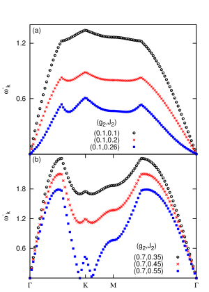
Figure 7: The magnon spectrum along symmetry directions in $1BZ$ for phase.I (Néel-$xy$). a) in going from phase.I to phase.III, b) in going from phase.I to phase.VI. Square symbols show the dispersion at the boundaries of this phase.

For the phase.I (Néel-$xy$), ${{{\bf{q}}}=0}$ and $\varphi=0$, then from Eqs.(LABEL:fk-mk), (44) and Eq.(LABEL:coeffs), one can calculate the magnon spectrum. For some values of the couplings $J_{2}$ and $g_{2}$ within the phase.I, the magnon dispersions are plotted along the symmetry directions in $1BZ$, shown in Fig. 7. The linear dispersion relation close to the $\Gamma$-point, in the bulk of this phase is the result of spontaneous breaking of in-plane $O_{2}$ symmetry leading to the formation of the Goldstone modes. The top panel of this figure shows that for small value of $g_{2}$, near the phase boundary with helical-$xy$ (phase.III), the linear dispersion tends to become quadratic, indicating the appearance of soft modes which tend to destabilize the Néel ordering. On the other hand, the bottom panel, represents the emergence of some zero modes at finite wave-vectors around the $K$-point, at the border of phase.I and phase.VI. The spectrum becomes non-real in passing from the phase.I to Phase.III at the $\Gamma$-point, and at some non-zero wave-vectors at the boundary of phase.I and phase.VI. Therefore, LSW method confirms the classical phase boundaries found in the previous section.

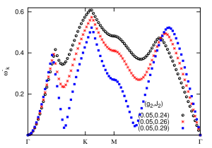
Figure 8: The magnon spectrum along symmetry directions in $1BZ$ for phase.III (helical-$xy$), in going from phase.III to phase.IV (helical-$xz$)

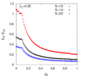
Figure 9: The ratio of quantum correction to classical energy ($E_{Q}/E_{cl}$) vs $g_{2}$, for $J_{2}=0.25$. The plots corresponds to $S=1/2,1,3/2$ from top to bottom, respectively.

In phase.III, we already discussed that the classical ground state is degenerate on a manifold determined by Eq.(24). However, the LSW analysis shows that only the spin state with the wave-vector

$${{{\bf{q}}}^{*}_{x}}=0$$

$${{{\bf{q}}}^{*}_{y}}=\frac{2}{\sqrt{3}a}\cos^{-1}\left({\frac{{J_{1}}^{2}}{16(J_{2}-g_{2})^{2}}}-\frac{5}{4}\right)$$ (46)

and the other five symmetrically equivalent by $\pi/6$ rotations (displayed by filled circles in Fig. 3), are stable against the quantum fluctuations, in a sense that their magnon spectrum are real over all $1BZ$. This is the manifestation of the quantum order-by-disorder, already been obtained for $J_{1}-J_{2}$ model aron2010 . Indeed, the quantum fluctuations select only the helical states along the nearest-neighbor directions. Fig. 8, exhibits the excitation dispersion in the bulk of phase.III for three sets of couplings $(g_{2},J_{2})$. The nonlinear dispersion near the $\Gamma$-points indicates the presence of the soft Goldstone modes in this phase. Close to the boundary with phase.IV, some zero modes tend to emerge which eventually destabilize the in-plane states.

In Fig. 9, the ratio of the zero point energy ($E_{Q}$) to the classical energy ($E_{cl}$), at fixed $J_{2}=0.25$, is depicted vs $g_{2}$ for the spin sizes $S=1/2,1,3/2$. This figure shows the increasing effect of quantum fluctuations when the spin size decreases. For $S=1/2$, in the helical-$xy$ phase, the quantum correction is in the order of the classical energy, hence it is possible that the helical states melt into some purely quantum states such as nematic staggered dimerized or plaquette valence bond states. Such a scenario has been proposed for $J_{1}-J_{2}$ model and a plaquette ordering was found for $1/6<J_{2}<0.3$ which transforms to a staggered dimerized state for $J_{2}>0.3$ mosadeq ; pvb2 .

IV.2 Phase.II

The magnetic unit cell of a state in phase.II (collinear-$z$) consists of four spins, two in up and two in down direction(Fig. 2). Thus, the primitive translational vectors for such a unit cell are $2{\bf a}$ and ${\bf b}$, and the corresponding first Brillouin zone is a rectangle rotated by $\pi/4$ ( Fig. 10). Here, we need four sets of bosonic operators for LSW analysis, as the following

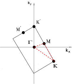
Figure 10: The first Brillouin of the magnetic unit cell corresponding to a spin configuration in phase.II, shown in Fig. 2

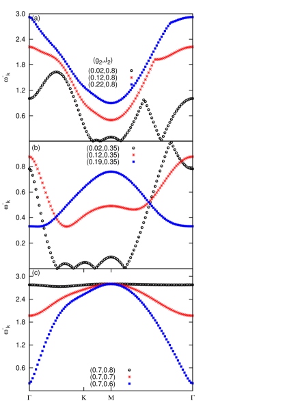
Figure 11: The magnon spectrum along symmetry directions in $1BZ$ for phase.II (Collinear-$z$). a) in going from phase.II to phase.V, b) in going from phase.II to phase.IV. c) in going from phase.II to phase.VI

$$\begin{array}[]{cc}\left\{\begin{array}[]{l}S_{\nu,i}^{+}\approx\hat{a}_{\nu,i}\sqrt{2S}\\ S_{\nu,i}^{-}\approx\hat{a}_{\nu,i}^{\dagger}\sqrt{2S}\\ S_{\nu,i}^{z}=S-\hat{a}_{\nu,i}^{\dagger}\hat{a}_{\nu,i}\\ \nu=1,3\end{array}\right.&~{}~{}~{}~{}\left\{\begin{array}[]{l}S_{\nu,i}^{+}\approx\hat{a}_{\nu,i}^{\dagger}\sqrt{2S}\\ S_{\nu,i}^{-}\approx\hat{a}_{\nu,i}\sqrt{2S}\\ S_{\nu,i}^{z}=\hat{a}_{\nu,i}^{\dagger}\hat{a}_{\nu,i}-S\\ \nu=2,4\end{array}\right.\end{array}$$

Using the above transformations, in the linear approximation we obtain the following quadratic Hamiltonian,

$$H_{\bf LSW}=E_{\rm cl}+S\sum_{{{\bf{k}}}>0}[\hat{\psi}_{{\bf{k}}}^{\dagger}H^{\phantom{\dagger}}_{{\bf{k}}}\hat{\psi}_{{\bf{k}}}-G].$$ (47)

in which

$$\hat{\psi}_{\textbf{k}}^{\dagger}=\begin{pmatrix}\hat{a}_{1\textbf{k}}^{{\dagger}}~{}\hat{a}_{2\textbf{k}}^{{\dagger}}~{}\hat{a}_{3\textbf{k}}^{{\dagger}}~{}\hat{a}_{4\textbf{k}}^{{\dagger}}~{}\par\hat{a}_{1-\textbf{k}}~{}\hat{a}_{2-\textbf{k}}~{}\hat{a}_{3-\textbf{k}}~{}\hat{a}_{4-\textbf{k}}\\ \end{pmatrix},$$ (48)

for the classical energy we have

$$E_{\rm cl} = -NS^{2}(\frac{J_{1}}{2}+J_{2}+g_{2}),$$ (49)

and $G$ is given by

$$G=+4J_{1}+8(J_{2}+g_{2}).$$ (50)

$H_{\bf k}$ is a $8\times 8$ matrix

$$H_{\textbf{k}}=\left(\begin{array}[]{cccccccc}D_{{\bf{k}}}&0&0&J_{1}&0&C_{\textbf{k}}^{*}&A_{\textbf{k}}^{*}&0\\ 0&D_{{\bf{k}}}&J_{1}&0&C_{{\bf{k}}}&0&0&B_{\textbf{k}}^{*}\\ 0&J_{1}&D_{\textbf{k}}&0&A_{\textbf{k}}&0&0&C_{\textbf{k}}\\ J_{1}&0&0&D_{\textbf{k}}&0&B_{\textbf{k}}&C_{\textbf{k}}^{*}&0\\ 0&C_{\textbf{k}}^{*}&A_{\textbf{k}}^{*}&0&D_{{\bf{k}}}&0&0&J_{1}\\ C_{\textbf{k}}&0&0&B_{\textbf{k}}^{*}&0&D_{{\bf{k}}}&J_{1}&0\\ A_{\textbf{k}}&0&0&C_{\textbf{k}}&0&J_{1}&D_{{\bf{k}}}&0\\ 0&B_{\textbf{k}}&C_{{\bf{k}}}^{*}&0&J_{1}&0&0&D_{{\bf{k}}},\\ \end{array}\right),$$ (51)

whose elements are as the following

$$A_{{\bf{k}}} = J_{1}(e^{ik_{a}}+e^{i(k_{a}+k_{b})})$$

$$B_{{\bf{k}}} = J_{1}(1+e^{ik_{b}})$$

$$C_{{\bf{k}}} = (J_{2}-g_{2})(1+e^{ik_{a}}+e^{-ik_{b}}+e^{i(k_{a}+k_{b})})$$

$$D_{{\bf{k}}} = J_{1}+2(J_{2}+g_{2})+2(J_{2}-g_{2})\cos(k_{b})$$

in which $k_{a}={2\bf k\cdot\bf a}$ and $k_{b}={\bf k\cdot\bf b}$.

Diagonalizing the matrix $H_{{\bf{k}}}$, for the lowest magnon dispersion, we get

$$\omega^{-}_{{\bf{k}}}=\frac{1}{2}\sqrt{\alpha_{{\bf{k}}}-2\beta_{{\bf{k}}}}$$ (53)

in which

$$\alpha_{{\bf{k}}} = 2(2-|B_{{\bf{k}}}|^{2}-|A_{{\bf{k}}}|^{2}-2|C_{{\bf{k}}}|^{2}+2{D_{{\bf{k}}}}^{2})$$

$$\beta_{{\bf{k}}} = [(A_{{\bf{k}}}A^{*}_{{\bf{k}}}-B_{{\bf{k}}}B^{*}_{{\bf{k}}})^{2}+4|A_{{\bf{k}}}C_{{\bf{k}}}^{*}+B_{{\bf{k}}}C_{{\bf{k}}}|^{2}$$

$$- 4|A_{{\bf{k}}}-B_{{\bf{k}}}^{*}|^{2}-8D_{{\bf{k}}}(C_{{\bf{k}}}(A_{{\bf{k}}}^{*}+B_{{\bf{k}}})$$

$$+ C_{{\bf{k}}}^{*}(A_{{\bf{k}}}+B_{{\bf{k}}}^{*}))+16D_{{\bf{k}}}^{2}]^{1/2}$$

The magnon dispersion for three sets of the couplings $(g_{2},J_{2})$ is plotted in Fig. 11. As can be seen from the top and middle panels of this figure, the appearance of zero modes at the borders of phase.V and phase.IV, indicates the instability of collinear-$z$ states at those boundaries. On the other hand the bottom panel, shows the appearance of Goldstone modes at the border of phase.II and phase.VI, indicating restoration of in-plane $O_{2}$ symmetry. The absence of the Goldstone modes at the boundaries with phases VI and V would be the sign of the breaking of all rotational symmetries at these two regions.

IV.3 Phase.IV and V

In the phase.IV (helical-$xz$) and phase.V (Non-coplanar), the $z$-component of the spins are incommensurate, i.e ${\acute{\bf{q}}}$ is not equal to any $M$-point, hence the coefficients of the Hamiltonian Eq.(36) are site dependent and Fourier transformation would not be useful to find its eigenvalues. For $g_{2}=0$ and $J_{2}>0.3$, it has been shown that an incommensurate planar state would be selected by quantum order by disorder mechanism aron2010 . Turning on the $g_{2}$ term, the planar states are confined to be on plane normal to the horizontal plane and as explained in Sec.II-B, these classical states possess $O_{2}$ rotational symmetry in the vertical plane. However the quantum fluctuations breaks the $O_{2}$ symmetry, and as a result the translational symmetry of the ${\bf{LSW}}$ Hamiltonian will be lost. The coefficients of the Hamiltonian, Eq.(36) are quasi-periodic, which can be considered as a random Hamiltonian with a long-range correlated disorder. Therefore, the localization of the magnons would be a possible scenario provided $g_{2}$ term be strong enough. In this case one expects the freezing of the spins in random directions and emergence of a spin-glass ground state. To investigate the localization of magnon, the exact diagonalization of the ${\bf{LSW}}$ Hamiltonian and also the methods such as level statistics and inverse participation ratio are required, and we leave this study for the future works. However, since $g_{2}$ is small for the range of couplings in the phase diagram ($g_{2}\lesssim 0.02$), it can be speculated that the magnon localization is not probable in these two phases and the helical states selected due to quantum order by disorder mechanism are still stable. Nevertheless, for $S=1/2$, the quantum fluctuations may destabilize such a helical state in favor of some valence bond configurations.

V Conclusion

In summary, we obtained the zero temperature phase diagram of the classical Kane-Mele-Heisenberg model. The competition among the isotropic exchange interactions between first $J_{1}$ and second neighbors $J_{2}$, as well as the second neighbor anisotropic exchange $g_{2}$, gives rise to a rich phase diagram. In the region of the couplings space where all the coupling are positive, we found six distinct phases. Three phases are long-range ordered, namely, in-plane Néel (phase.I), commensurate vertical planar (phase.VI) and vertical collinear (phase.II). The other three, being infinitely degenerate due to the frustrating competition between the couplings, are incommensurate in-plane helical (phase.III), incommensurate vertical planar (phase.VI) and incommensurate non-coplanar (phase.V). The linear spin wave analysis, done analytically in phase.III, shows that the quantum order-by-disorder is at work in this phase, and a set of rotationally equivalent helical state are selected from the ground state manifold, by the quantum fluctuations. In the phases IV and V, due the lack of translational symmetry in the LSW Hamiltonian, the analytic calculations is not possible and numeric exact diagonalization of the Hamiltonian is required to figure out how the quantum fluctuations affect the classical ground states in these regions. This is the subject of our current research.

It is also found that for $S=1/2$, the quantum correction to the ground state energy is at the same order as the classical energy, hence the selected helical states are likely to melt down into some purely quantum ground state. Whether the emergent phase is a QSL or a kind of plaquette valence bond or else, one needs to employ the methods such as exact diagonalization, variational Monte Calro, bond operator formalism which may shed more light on the nature of the quantum ground state in the phase as well as the phases IV and V.

As the final remark, we add that the methods employed in this paper can be used for obtaining the phase diagram of the spin systems in which the axial spin symmetry is also broken. Such models are realized in monolayers of Sodium Iridate ($Na_{2}IrO_{3}$ ), where the next nearest hopping term in its tight-binding model is link dependent due to dependence of intrinsic spin-orbit coupling to the hopping direction shitade . The spin Hamiltonian arising in the strong coupling limit of this model is recently investigated and shown to have a rich phase diagram Rachel ; Kargarian . The complete breaking of the spin $SU(2)$ symmetry also occurs when a Rashba spin-orbit coupling is added to the KM model, leading to a link dependent exchange interaction in the large coupling limit Rachel . The classical phase diagrams of aforementioned models are currently under investigation in our group.

Appendix A Matrix elements of LSW Hamiltonian in real space

The matrices introduced the spin-wave Hamiltonian Eq.(36) are defined as

$$M_{i}=\begin{pmatrix}\epsilon^{i}_{1}&0&0&0\\ 0&\epsilon^{i}_{2}&0&0\\ 0&0&\epsilon^{i}_{1}&0\\ 0&0&0&\epsilon^{i}_{2}\end{pmatrix}$$ (55)

and

$$T_{ij}=\begin{pmatrix}{t^{ij}_{1}}&{t^{ij}_{5}}&{t^{ij}_{3}}&{t^{ij}_{6}}\\ {t^{ij}_{5}}^{*}&{{t^{ij}_{2}}}&{{t^{ij}_{6}}}^{*}&{{t^{ij}_{4}}}\\ {{t^{ij}_{3}}}^{*}&{{t^{ij}_{6}}}^{*}&{{t^{ij}_{1}}}^{*}&{{t^{ij}_{5}}}^{*}\\ {{t^{ij}_{6}}}&{{t^{ij}_{4}}}^{*}&{{t^{ij}_{5}}}&{{{t^{ij}_{2}}}^{*}},\end{pmatrix}$$ (56)

whose elements are given by

$$\epsilon^{i}_{1} = -2\chi_{3}+{t^{ij}_{7}}$$

$$\epsilon^{i}_{2} = -2\chi_{4}+{t^{ij}_{7}}$$

$${t^{ij}_{1}} = \chi_{1}+\chi_{5}+i\chi_{6}-i\chi_{7}$$

$${t^{ij}_{2}} = \chi_{2}+\chi_{5}-i\chi_{8}+i\chi_{9}$$

$${t^{ij}_{3}} = \chi_{1}-\chi_{5}-i\chi_{6}-i\chi_{7}$$

$${t^{ij}_{4}} = \chi_{2}-\chi_{5}+i\chi_{8}+i\chi_{9}$$

$${t^{ij}_{5}} = \frac{J_{1}}{2}[(\zeta_{1}-1)\cos({{\bf{q}}}\cdot\delta_{1}-\phi)+\zeta_{2}-i\zeta_{3}-i\zeta_{4}]$$

$${t^{ij}_{6}} = \frac{J_{1}}{2}[(\zeta_{1}+1)\cos({{\bf{q}}}\cdot\delta_{1}-\phi)+\zeta_{2}+i\zeta_{3}-i\zeta_{4}]$$

$${t^{ij}_{7}} = J_{1}[\zeta_{1}+\zeta_{2}\cos({{\bf{q}}}\cdot\delta_{1}-\phi)],$$

where

$$\zeta_{1} = \frac{1}{2}[\cos(\acute{{{\bf{q}}}}\cdot\delta_{1}+\gamma-\eta)$$

$$+ \cos(2\acute{{{\bf{q}}}}\cdot{{\bf{r}}}_{i}+\acute{{{\bf{q}}}}\cdot\delta_{1}+\gamma+\eta)]$$

$$\zeta_{2} = \frac{1}{2}[\cos(\acute{{{\bf{q}}}}\cdot\delta_{1}+\gamma-\eta)$$

$$- \cos(2\acute{{{\bf{q}}}}\cdot{{\bf{r}}}_{i}+\acute{{{\bf{q}}}}\cdot\delta_{1}+\gamma+\eta)]$$

$$\zeta_{3} = \sin({{\bf{q}}}\cdot\delta_{1}-\phi)\cos(\acute{{{\bf{q}}}}\cdot{{\bf{r}}}_{i}+\gamma)$$

$$\zeta_{4} =- \sin({{\bf{q}}}\cdot\delta_{1}-\phi)\cos(\acute{{{\bf{q}}}}\cdot{{\bf{r}}}_{i}+\acute{{{\bf{q}}}}\cdot\delta_{1}+\eta)$$

$$\chi_{1} = \frac{(J_{2}-g_{2})}{2}\cos({{\bf{q}}}\cdot\delta_{2})[\cos(\acute{{{\bf{q}}}}\cdot\delta_{2})$$

$$+ \cos(2\acute{{{\bf{q}}}}\cdot{{\bf{r}}}_{i}+\acute{{{\bf{q}}}}\cdot\delta_{2}+2\gamma)]$$

$$+ \frac{(J_{2}+g_{2})}{2}[\cos(\acute{{{\bf{q}}}}\cdot\delta_{2})-\cos(2\acute{{{\bf{q}}}}\cdot{{\bf{r}}}_{i}+\acute{{{\bf{q}}}}\cdot\delta_{2}+2\gamma)]$$

$$\chi_{2} = \frac{(J_{2}-g_{2})}{2}\cos({{\bf{q}}}\cdot\delta_{2})[\cos(\acute{{{\bf{q}}}}\cdot\delta_{2})$$

$$+ \cos(2\acute{{{\bf{q}}}}\cdot{{\bf{r}}}_{i}+\acute{{{\bf{q}}}}\cdot\delta_{2}+2\eta)]$$

$$+ \frac{(J_{2}+g_{2})}{2}[\cos(\acute{{{\bf{q}}}}\cdot\delta_{2})-\cos(2\acute{{{\bf{q}}}}\cdot{{\bf{r}}}_{i}+\acute{{{\bf{q}}}}\cdot\delta_{2}+2\eta)]$$

$$\chi_{3} = \frac{(J_{2}-g_{2})}{2}\cos({{\bf{q}}}\cdot\delta_{2})[\cos(\acute{{{\bf{q}}}}\cdot\delta_{2})$$

$$- \cos(2\acute{{{\bf{q}}}}\cdot{{\bf{r}}}_{i}+\acute{{{\bf{q}}}}\cdot\delta_{2}+2\gamma)]$$

$$+ \frac{(J_{2}+g_{2})}{2}[\cos(\acute{{{\bf{q}}}}\cdot\delta_{2})+\cos(2\acute{{{\bf{q}}}}\cdot{{\bf{r}}}_{i}+\acute{{{\bf{q}}}}\cdot\delta_{2}+2\gamma)]$$

$$\chi_{4} = \frac{(J_{2}-g_{2})}{2}\cos({{\bf{q}}}\cdot\delta_{2})[\cos(\acute{{{\bf{q}}}}\cdot\delta_{2})$$

$$- \cos(2\acute{{{\bf{q}}}}\cdot{{\bf{r}}}_{i}+\acute{{{\bf{q}}}}\cdot\delta_{2}+2\eta)]$$

$$+ \frac{(J_{2}+g_{2})}{2}[\cos(\acute{{{\bf{q}}}}\cdot\delta_{2})+\cos(2\acute{{{\bf{q}}}}\cdot{{\bf{r}}}_{i}+\acute{{{\bf{q}}}}\cdot\delta_{2}+2\eta)]$$

$$\chi_{5} = (J_{2}-g_{2})\cos({{\bf{q}}}\cdot\delta_{2})$$

$$\chi_{6} = (J_{2}-g_{2})\sin({{\bf{q}}}\cdot\delta_{2})\cos(\acute{{{\bf{q}}}}\cdot{{\bf{r}}}_{i}+\gamma)$$

$$\chi_{7} =- (J_{2}-g_{2})\sin({{\bf{q}}}\cdot\delta_{2})\cos(\acute{{{\bf{q}}}}\cdot{{\bf{r}}}_{i}+\acute{{{\bf{q}}}}\cdot\delta_{2}+\gamma)$$

$$\chi_{8} = (J_{2}-g_{2})\sin({{\bf{q}}}\cdot\delta_{2})\cos(\acute{{{\bf{q}}}}\cdot{{\bf{r}}}_{i}+\eta)$$

$$\chi_{9} =- (J_{2}-g_{2})\sin({{\bf{q}}}\cdot\delta_{2})\cos(\acute{{{\bf{q}}}}\cdot{{\bf{r}}}_{i}+\acute{{{\bf{q}}}}\cdot\delta_{2}+\eta)$$

References

- (1) Z. Y. Meng, T. C. Lang, S. Wessel, F. F. Assaad, A. Muramatsu, Nature 464 847 (2010).
- (2) S. Sorella, Y. Otsuka, and S. Yunoki, Scientific Reports 2, 992 (2012);
- (3) F.F. Assaad, and I.F. Herbut, arXiv:1304.6340.
- (4) B. K. Clark, arXiv:1305.0278.
- (5) S. Okumura, H. Kawamura, T. Okubo, and Y. Motome, J. Phys. Soc. Jpn. 79, 114705 (2010).
- (6) A. Mulder, R. Ganesh, L. Capriotti, and A. Paramekanti, 81, 214419 (2010).
- (7) J. Oitmaa, R. R. P. Singh, Phys. Rev. B 85, 014428 (2012).
- (8) H. Mosadeq, F. Shahbazi, and S. A. Jafari, J. Phys. Condens. Matter, 23, 226006 (2011).
- (9) A. F. Albuquerque, D. Schwandt, B. Hetenyi, S. Capponi, M. Mambirini, A. M. Lauchli, Phys. Rev. B 84, 024406 (2011).
- (10) J. Reuther, D. A. Abanin, T. Thomale, Phys. Rev. B 84, 014417 (2011).
- (11) P. H. Y. Li, R. F. Bishop, D. J. J. Farnell, and C. E. Campbell, J. Phys.: Condens. Matter 24, 236002 (2012);Phys. Rev. B 86, 144404 (2012)..
- (12) R. Ganesh, S. Nishimoto, and J. van den Brink, Phys. Rev. B 87, 054413 (2013).
- (13) Z. Zhu, D. A. Huse, and S. R. White, Phys. Rev. Lett. 110, 127205 (2013).
- (14) R. F. Bishop, P. H. Y. Li, and C. E. Campbell, arXiv:1303.5249.
- (15) D. C. Cabra, C. A. Lamas, and H. D. Rosales Phys. Rev. B 83, 094506 (2011).
- (16) F. Wang, Phys. Rev. B 82, 024419 (2010).
- (17) Y-M. Lu, Y. Ran, and P. A. Lee, Phys. Rev. B 83, 224413 (2011).
- (18) Y-M. Lu, and Y. Ran, Phys. Rev. B 84, 024420 (2011).
- (19) B. K. Clark, D. A. Abanin, S. L. Sondhi, Phys. Rev. Lett. 107, 087204 (2011).
- (20) H. Zhang, and C. A. Lamas, Phys. Rev. B 87, 024415 (2013).
- (21) X-L. Yu, D-Y Liu, P. Li, and L-J. Zou, arXiv:1301.5282.
- (22) F. Mezzacapo, and M. Boninsegni, Phys. Rev. B 85, 060402 (2012).
- (23) H-Y. Yang, A.F. Albuquerque, S. Capponi, A.M. Lauchli, K.P. Schmidt, New J. Phys. 14, 115027 (2012).
- (24) K. Damle, F. Alet, and S. Pujari, arXiv:1302.1408.
- (25) J. D. Reger, J. A. Riera, and A. P. Young, J. Phys.: Condens. Matter 1, 1855 (1989).
- (26) J. Oitmaa, C. J. Hamer, and Z. Weihong, Phys. Rev. B 45, 9834 (1992).
- (27) Z. Noorbakhsh, F. Shahbazi, S. A. Jafari, G. Baskaran, J. Phys. Soc. Jpn. 78, 054701 (2009).
- (28) M. Z. Hasan, and C. L. Kane, Rev. Mod. Phys 82, 3045 (2010).
- (29) X-L. Qi, and S-C. Zhang, Rev. Mod. Phys 83, 1057 (2011).
- (30) M. Hohenadler, and F. F. Assaad, J. Phys.: Condes. Matter 25, 143201 (2013).
- (31) C. L. Kane and E. J. Mele, Phys. Rev. Lett 95, 226801 (2005).
- (32) S. Rachel and K. L. Hur, Phys. Rev. B 82, 075106 (2010).
- (33) Y. Yamaji, and M. Imada, Phys. Rev. B 83, 205122 (2011).
- (34) D. Zheng, G-M. Zhang, and C. Wu, Phys. Rev. B 84, 205121 (2011).
- (35) J. Wen, M. Kargarian, A. Vaezi, and G. A. Fiete, Phys. Rev. B 84, 235149 (2011).
- (36) M. Hohenadler, T. C. Lang, F. F. Assaad, Phys. Rev. Lett. 106, 100403 (2011).
- (37) S-L. Yu, X.C. Xie, and J-X. Li, Phys. Rev. Lett. 107, 010401 (2011).
- (38) M. Mardani, M.S. Vaezi, and A. Vaezi, arXiv:1111.5980.
- (39) M. Hohenadler, Z. Y. Meng, T. C. Lang, S. Wessel, A. Muramatsu, and F. F. Assaad, Phys. Rev. B 85, 115132 (2012).
- (40) W. Wu, S. Rachel, W-M. Liu, K. L. Hur, Phys. Rev. B 85, 205102 (2012).
- (41) C. Griset, and C. Xu, Phys. Rev. B 85, 045123 (2012).
- (42) A. Vaezi, M. Mashkoori, M. Hosseini, Phys. Rev. B 85, 195126 (2012).
- (43) E. Rastelli, A. Tassi, and L. Reatto, Physica B 97, 1 (1979).
- (44) J. B. Fouet, P. Sindzingre, and C. Lhuillier, European Physical Journal B 20, 241 (2001).
- (45) J. M. Luttinger and L. Tisza, Phys. Rev. 70, 954 (1946).
- (46) D. H. Lyons and T. A. Kaplan, Phys. Rev. 120, 1580 (1960).
- (47) T. A. Kaplan and N. Menyuk, Phil. Mag. 87, 3711 (2006).
- (48) S. R. Sklan and C. L. Henley, preprint (arXiv:1209.1381).
- (49) M. F. Lapa and C. L. Henley, preprint (arXiv:1210.6810).
- (50) S. Wolfram, The Mathematica Book (Wolfram Media,2003), 5th ed.
- (51) L. R. Walker and R. E. Walstedt, Phys. Rev. Lett. 38, 514 (1977).
- (52) S. J. Miyake, J. Phys. Soc. Jap 61, 983 (1992).
- (53) R. R. P. Singh and D. A. Huse, Phys. Rev. Lett. 68, 1766 (1992).
- (54) T. Holstein and H. Primakoff, Phys. Rev. 58, 1098 (1940).
- (55) P. W. Anderson, Phys. Rev. 86, 694 (1952).
- (56) A. Auerbach, Interacting Electrons and Quantum Magnetism, (Springer-Verlag, New York, 1994).
- (57) A. Shitade, H. Katsura, J. Kunes, X.-L. Qi, S.-C. Zhang, and N. Nagaosa, Phys. Rev. Lett. 102, 256403 (2009).
- (58) J. Reuther, R. Thomale, S. Rachel, Phys. Rev. B 86, 155127 (2012).
- (59) M. Kargarian, A. Langari, G. A. Fiete, Phys. Rev. B 86, 205124 (2012).