Cosmology with a decaying vacuum

Abstract

Properties of unstable false vacuum states are analyzed from the point of view of the quantum theory of unstable states. Some of false vacuum states survive up to times when their survival probability has a non-exponential form. At times much latter than the transition time, when contributions to the survival probability of its exponential and non-exponential parts are comparable, the survival probability as a function of time t has an inverse power-like form. We show that at this time region the instantaneous energy of the false vacuum states tends to the energy of the true vacuum state as $1/t^{2}$ for $t\to\infty$.

1 Introduction

A discussion of the decay of the false vacuum was began in two pioneer papers by Coleman and, Callan and Coleman Coleman ; Callan . ”The fate of the false vacuum” was discussed there, namely the unstability of a physical system in a state which is not an absolute minimum of its energy density, and which is separated from the minimum by an effective potential barrier. It was shown, in those papers, that even if the state of the early Universe is too cold to activate a ”thermal” transition (via thermal fluctuations) to the lowest energy (i.e. ”true vacuum”) state, a quantum decay from the false vacuum to the true vacuum may still be possible through a barrier penetration via macroscopic quantum tunneling. Not long ago, the decay of the false vacuum state in a cosmological context has attracted renewed interest, especially in view of its possible relevance in the process of tunneling among the many vacuum states of the string landscape (a set of vacua in the low energy approximation of string theory).

Since the work of Khalfin Khalfin it is known that for long times compared to the characteristic decay time of an unstable state (when the decay law has an exponential form), the survival probability of such states is no longer described by an exponential function of time $t$ but it decreases as $t\rightarrow\infty$ more slowly than any exponential function of $t$. Krauss and Dent analyzing a false vacuum decay Krauss ; Winitzki pointed out that in eternal inflation, even though regions of false vacua by assumption should decay exponentially, gravitational effects force space in a region that has not decayed yet to grow exponentially fast. This effect causes that many false vacuum regions can survive up to the times much later than times when the exponential decay law holds. In the mentioned paper by Krauss and Dent the attention was focused on the possible behavior of the unstable false vacuum at very late times, where deviations from the exponential decay law become to be dominat. In our paper the attention will be focussed on properties of decaying false vacuum states from the point of view of the quantum theory of unstable states evolving in time and decaying. It will be shown that at late times the instantaneous energy of the false vacuum states tends to the energy of the true vacuum state as $1/t^{2}$ for $t\to\infty$. This means that in the case of such false vacuum states the cosmological constant becomes time depending. Next effective cosmological model with obtained decaying Lambda term will be studied in details.

2 Unstable states in short

If $|M\rangle$ is an initial unstable state then the survival probability, ${\cal P}(t)$, equals ${\cal P}(t)=|A(t)|^{2}$, where $A(t)$ is the survival amplitude, $A(t)=\langle M|M;t\rangle,\;\;\;{\rm and}\;\;\;a(0)=1$, and $[|M;t\rangle=\exp\,[-itH]\,|M\rangle$, $H$ is the total Hamiltonian of the system under considerations. The spectrum, $\sigma(H)$, of $H$ is assumed to be bounded from below, $\sigma(H)=[E_{min},\infty)$ and $E_{min}>-\infty$.

From basic principles of quantum theory it is known that the amplitude $A(t)$, and thus the decay law ${\cal P}_{M}(t)$ of the unstable state $|M\rangle$, are completely determined by the density of the energy distribution function $\omega({E})$ for the system in this state

$$A(t)=\int_{Spec.(H)}\omega({E})\;e^{\textstyle{-\frac{i}{\hbar}\,{E}\,t}}\,d{E}.$$ (1)

where $\omega({E})\geq 0$ and $\omega({E})=0$ for $E<E_{min}$. From this last condition and from the Paley–Wiener Theorem it follows that there must be (see Khalfin ) $|A(t)|\;\geq\;A_{1}\,\exp[-A_{2}\,t^{q}]$, for $|t|\rightarrow\infty$. Here $A_{1}>0,\,A_{2}>0$ and $0<q<1$.

This means that the decay law ${\cal P}_{M}(t)$ of unstable states decaying in the vacuum can not be described by an exponential function of time $t$ if time $t$ is suitably long, $t\rightarrow\infty$, and that for these lengths of time ${\cal P}_{M}(t)$ tends to zero as $t\rightarrow\infty$ more slowly than any exponential function of $t$.

The analysis of the models of the decay processes shows that ${\cal P}_{M}(t)\simeq\exp[-\frac{\Gamma_{M}t}{\hbar}]$, (where $\Gamma_{M}$ is the decay rate of the state $|M\rangle$), to an very high accuracy at the canonical decay times $t$: From $t$ suitably later than the initial instant $t_{0}$ up to $t\gg\tau_{M}=\hbar/{\Gamma_{M}}$ and smaller than $t=T$, where $T$ is the crossover time and denotes the time $t$ for which the non–exponential deviations of $A(t)$ begin to dominate.

In general, in the case of quasi–stationary (metastable) states it is convenient to express $A(t)$ in the following form

$$A(t)=A_{exp}(t)+A_{non}(t),$$ (2)

where $A_{exp}(t)$ is the exponential part of $A(t)$, that is $A_{exp}(t)=\exp[-it(E_{M}-\frac{i}{2}\,\Gamma_{M})]$, ($E_{M}$ is the energy of the system in the state $|M\rangle$ measured at the canonical decay times, $N$ is the normalization constant), and $A_{non}(t)$ is the non–exponential part of $A(t)$. For times $t\sim\tau_{M}$: $|A_{exp}(t)|\gg|A_{non}(t)|$,

The crossover time $T$ can be found by solving the following equation,

$$|A_{exp}(t)|^{\,2}=|A_{non}(t)|^{\,2}.$$ (3)

The amplitude $A_{non}(t)$ exhibits inverse power–law behavior at the late time region: $t\gg T$. Indeed, the integral representation (1) of $A(t)$ means that $A(t)$ is the Fourier transform of the energy distribution function $\omega(E)$. Using this fact we can find asymptotic form of $A(t)$ for $t\rightarrow\infty$. Results are rigorous.

Let us consider $\omega({E})$ having universal and general form. Namely let $\omega({E})$ be of the form

$$\omega({E})=({E}-{E}_{min})^{\lambda}\;\eta({E})\;\in\;L_{1}(-\infty,\infty),$$ (4)

where $0<\lambda<1$ and it is assumed that $\eta(E_{min})>0$ and derivatives $\eta^{(k)}({E})$, ($k=0,1,\ldots,n$), exist and they are continuous in $[{E}_{min},\infty)$, and limits $\lim_{{E}\rightarrow{E}_{min}+}\;\eta^{(k)}({E})$ exist, $\lim_{{E}\rightarrow\infty}\;({E}-{E}_{min})^{\lambda}\,\eta^{(k)}({E})=0$ for all above mentioned $k$, then

$$A(t) \begin{array}[]{c}{}\hfil\\ \sim\\ \scriptstyle{t\rightarrow\infty}\end{array} (-1)\,e^{\textstyle{-\frac{i}{\hbar}{E}_{min}t}}\;\Big{[}\Big{(}-\frac{i\hbar}{t}\Big{)}^{\lambda+1}\times$$

$$\times\;\Gamma(\lambda+1)\;\eta_{0}\;$$

$$+\;\lambda\,\Big{(}-\frac{i\hbar}{t}\Big{)}^{\lambda+2}\times$$

$$\times\;\Gamma(\lambda+2)\;\eta_{0}^{(1)}\;+\;\ldots\Big{]}=A_{non}(t).$$

3 Energy and decay rate

The amplitude $A(t)$ contains information about the decay law ${\cal P}_{M}(t)$ of the state $|M\rangle$, that is about the decay rate $\Gamma_{M}$ of this state, as well as the energy ${E}_{M}$ of the system in this state. This information can be extracted from $A(t)$. Indeed if $|M\rangle$ is an unstable (a quasi–stationary) state then $A(t)\cong\exp[\frac{i}{\hbar}({E}_{M}-\frac{i}{2}\Gamma_{M})\,t]$. So, there is

$${E}_{M}-\frac{i}{2}\Gamma_{M}\equiv i\hbar\,\frac{\partial A(t)}{\partial t}\;\frac{1}{A(t)},$$ (10)

in the case of quasi–stationary states.

Taking the above into account one can define the ”effective Hamiltonian”, $h_{M}$, for the one–dimensional subspace of states ${\cal H}_{||}$ spanned by the normalized vector $|M\rangle$ as follows

$$h_{M}\stackrel{{\scriptstyle\rm def}}{{=}}i\hbar\,\frac{\partial A(t)}{\partial t}\;\frac{1}{A(t)}.$$ (11)

In general, $h_{M}$ can depend on time $t$, $h_{M}\equiv h_{M}(t)$. One meets this effective Hamiltonian when one starts with the Schrödinger Equation for the total state space ${\cal H}$ and looks for the rigorous evolution equation for the distinguished subspace of states ${\cal H}_{||}\subset{\cal H}$. Details can be found in EPJD-2009 and in CEJP-2009 . Thus, one finds the following expressions for the energy and the decay rate of the system in the state $|M\rangle$ under considerations, to be more precise for the instantaneous energy ${\cal E}_{M}(t)$ and the instantaneous decay rate, $\gamma_{M}(t)$, ${\cal E}_{M}\equiv{\cal E}_{M}(t)=\Re\,(h_{M}(t))$, $\gamma_{M}\equiv\gamma_{M}(t)=-\,2\,\Im\,(h_{M}(t))$, where $\Re\,(z)$ and $\Im\,(z)$ denote the real and imaginary parts of $z$ respectively.

Using (11) one can find that ${\cal E}_{M}(t\sim\tau_{M})\simeq{E}_{M}\neq{\cal E}_{M}(0)$, $\gamma_{M}(t\sim\tau_{M})\simeq\Gamma_{M}$, i. e., there is ${\cal E}_{M}(t)=E_{M}$ at the canonical decay time.

Starting from the asymptotic expression (2) for $A(t)$ and using (11) after some algebra one finds for times $t\gg T$ that

$${h_{M}(t)\vline}_{\,t\rightarrow\infty}\simeq{E}_{min}+(-\,\frac{i\hbar}{t})\,c_{1}\,+\,(-\,\frac{i\hbar}{t})^{2}\,c_{2}\,+\,\ldots,$$ (12)

where $c_{i}=c_{i}^{\ast},\;\;i=1,2,\ldots$; (coefficients $c_{i}$ depend on $\omega(E)$). This last relation means that

$${\cal E}_{M}(t) \simeq E_{min}\,+\,\frac{c_{2}}{t^{2}}\ldots,\;\;\;({\rm for}\;\;t\gg T).$$ (13)

(Here $c_{2}>0$). These properties take place for all unstable states which survived up to times $t\gg T$. From (13) it follows that $\lim_{t\rightarrow\infty}\,{\cal E}_{M}(t)=E_{min}$.

4 Cosmological applications

Krauss and Dent in their paper Krauss mentioned earlier made a hypothesis that some false vacuum regions do survive well up to the time $T$ or later. Let $|M\rangle=|0\rangle^{false}$, be a false,$|0\rangle^{true}$ – a true, vacuum states and $E^{false}_{0}$ be the energy of a state corresponding to the false vacuum measured at the canonical decay time and $E^{true}_{0}$ be the energy of true vacuum (i.e. the true ground state of the system). As it is seen from the results presented in previous Section, the problem is that the energy of those false vacuum regions which survived up to $T$ and much later differs from $E^{false}_{0}$, (see PRL-2011 and references one can find therein).

Going from quantum mechanics to quantum field theory one should take into account among others a volume factors so that survival probabilities per unit volume per unit time should be considered. The standard false vacuum decay calculations shows that the same volume factors should appear in both early and late time decay rate estimates (see Krauss ). This means that the calculations of cross–over time $T$ can be applied to survival probabilities per unit volume. For the same reasons within the quantum field theory the quantity ${\cal E}_{M}(t)$ can be replaced by the energy per unit volume $\rho_{M}$ because these volume factors appear in the numerator and denominator of the formula (10) for $h_{M}(t)$. Now, if one assumes that $E^{true}_{0}\equiv E_{min}$ then one has for the energy of the false vacuum state that at $t\gg T$,

$${\cal E}^{false}_{0}(t)\simeq E^{true}_{0}+\frac{c_{2}}{t^{2}}\ldots\;\;\neq\,E^{false}_{0}.$$ (15)

This property of the false vacuum states means that

$${\cal E}^{false}_{0}(t)\rightarrow E^{true}_{0}\;\;\;{\rm as}\;\;t\to\infty.$$ (16)

The basic physical factor forcing the wave function $|M;t\rangle$ and thus the amplitude $A(t)$ to exhibit inverse power law behavior at $t\gg T$ is a boundedness from below of $\sigma(H)$. This means that if this condition takes place and $\int_{-\infty}^{+\infty}\omega(E)\,dE\,<\,\infty$, then all properties of $A(t)$, including a form of the time–dependence at $t\gg T$, are the mathematical consequence of them both. The same applies by (11) to properties of $h_{M}(t)$ and concerns the asymptotic form of $h_{M}(t)$ and thus of ${\cal E}_{M}(t)$ and $\gamma_{M}(t)$ at $t\gg T$.

Note that properties of $A(t)$ and $h_{M}(t)$ discussed above do not take place when $\sigma(H)=(-\infty,+\infty)$. The late time behavior of the energy of the system in the false vacuum state,

$${\cal E}^{false}_{0}(t)\simeq E^{true}_{0}+\frac{c_{2}}{t^{2}}\ldots,\;\;\;{\rm for}\;\;\;t\gg T,$$ (17)

or, of the energy density $\rho^{false}_{0}(t)$:

$${\rho}^{false}_{0}(t)\simeq\rho^{true}_{0}+\frac{d_{2}}{t^{2}}\ldots,\;\;\;{\rm for}\;\;\;t\gg T,$$ (18)

(where $d_{i}=d_{i}^{\ast},\,i=,1,2,\ldots$), is the pure quantum effect following from the basic principles of the quantum theory. The standard relation is $\rho_{0}^{true}=\frac{\Lambda}{8\pi G}=\rho_{bare}$.

5 False vacuum cosmology

Let us take into account properties of the false vacuum described by the last relations and let us consider the cosmological model which is homogeneous and isotropic (possesses the Robertson - Walker metric) in which energy density of dark sector is given by the relation which consists of the bare cosmological constant $\Lambda$ and the term depending on the cosmological time $t$

$$\rho=\rho_{\text{de}}=\Lambda+\frac{\alpha^{2}}{t^{2}}.$$ (19)

As it is well know the Friedmann-Robertson-Walker model has a first integral which does not depend on the pressure $p$ and is given in the form called the Friedmann equation

$$3H^{2}=\rho_{\text{de}}+\rho_{\text{m}},$$ (20)

where $H=\frac{d\ln a}{dt}$ is the Hubble parameter, $t$ is the cosmological time and $a=a(t)$ is a scale factor.

For simplicity we assume that space is flat and matter is in the form of dust ($p=0$), so $\rho\equiv\rho_{m}=\rho_{\text{m},0}\;a^{-3}$ describes a dependence of the energy density of the matter on a scale factor or a redshift $z\colon 1+z=a^{-1}$. Therefore (19) and (20) give

$$\frac{\rho_{\text{m},0}a^{-3}}{3H^{2}}+\frac{\Lambda}{3H^{2}}+\frac{\alpha^{2}/t^{2}}{3H^{2}}\equiv 1.$$ (21)

Next we introduce the state variables ($x$, $y$, $z$) defined as $\sqrt{\Omega_{\text{m}}}=x\equiv\sqrt{\frac{\rho_{\text{m},0}a^{-3}}{3H^{2}}}$, $\sqrt{\Omega_{\Lambda}}=y\equiv\sqrt{\frac{\Lambda}{3H^{2}}}$ and $\sqrt{\Omega_{\alpha}}=z\equiv\sqrt{\frac{\alpha^{2}/t^{2}}{3H^{2}}}$. The quantities $x$, $y$, $z$ has the cosmological sense of density parameters for a matter, the cosmological constant and for the which mimics time dependence of the false decaying vacuum. The cosmological constant $\Lambda$ is assumed to be positive. Above variables, of course, satisfy the constrain $x^{2}+y^{2}+z^{2}=1$. Using this constrain after some algebra we obtain for state variables $(x,y,z)$ dynamical system in the phase space $(x,y,z)\colon x^{2}+y^{2}+z^{2}=1$, (i.e. on the unit sphere), having the following form:

$$\frac{dx}{d\tau} =x\left(\frac{3}{2}x^{2}+\frac{\sqrt{3}}{\alpha}z^{3}-\frac{3}{2}\right)$$ (22)

$$\frac{dy}{d\tau} =y\left(\frac{3}{2}x^{2}+\frac{\sqrt{3}}{\alpha}z^{3}\right)$$ (23)

$$\frac{dz}{d\tau} =z\left(-\frac{\sqrt{3}}{2}z+\frac{3}{2}x^{2}+\frac{\sqrt{3}}{\alpha}z^{3}\right),$$ (24)

where $z=\pm\sqrt{1-x^{2}-y^{2}}$ and the cosmological time $t$ is reparametrized to the new time parameter $\tau$ which is a monotonic function of $t$, i.e., $\tau\equiv\ln a$. The above system has three 2D invariant submanifolds: $\{x=0\}$, $\{y=0\}$, $\{z=0\}$ and the following critical points:

1. $x=1$, $y=0$, $z=0$ (Einstein-de Sitter universe),

2. $x=0$, $y=1$, $z=0$ (de Sitter stationary universe),

3. $z=1$, $x=0$, $y=0$ (Milne universe),

4. $y=0$, $x=\frac{1}{2}\sqrt{4-3\alpha^{2}}$, $z=\frac{1}{2}\sqrt{3\alpha^{2}}$ (Einstein-de Sitter dominated by the time-dependent part of the cosmological constant).

If we eliminate one state variables from the constraint condition then model dynamics constitute the 2D dynamical system and then right-hand sides of the system (22) — (24) are not given in the polynomial forms. In neighborhood of initial singularity the generic solution is representing $\Lambda$CDM universe dominating. There is a new critical point representing by a node and saddle point representing the Milne universe (without the horizon). In this case $a=a_{0}t$ and we have an unstable invariant submanifold, which is 2D if $\alpha\gg 1$, and an unstable node if $\alpha\ll 1$. For the late time ($t\rightarrow\infty$) the trajectories of the system are going to the Sitter universe like for the FRW model with the bare cosmological constant.

From dynamical analysis of the system one can observe how changes the critical points as well as its type. There are present bifurcation as the value of $\alpha$ parameter changes. For example the bifurcation value of $\alpha_{\text{bif}}$ for the critical point (4) is: $\alpha_{\text{bif}}=\frac{2}{\sqrt{3}}$.

Figure 1: A phase portrait of the system (22)-(24) for $\alpha=1$. There are three critical points at a finite domain labeled as (7), (1), (6) and four critical points at the boundary $x^{2}+y^{2}=1$. Notations: (1) the Milne universe dominated by the time dependent part of the cosmological constant; (2) the Einstein – de Sitter universe dominated by matter; (4) the de Sitter universe dominated by the bare $\Lambda$; (6) the Einstein-de Sitter universe dominated by the time dependent part of the cosmological constant.

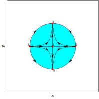
Figure 2: A phase portrait of the system (22)-(24) for $\alpha=2$.On the phase portrait there is one critical point at finite domain of saddle type and four critical points located at the boundary $\Omega_{m}+\Omega_{\Lambda}=1$.

Conclusions

We have shown that at late times, $t\gg T$, the energy of the false vacuum behaves as follows:

$${\cal E}^{false}_{0}(t)\simeq E^{true}_{0}+\frac{c_{2}}{t^{2}}\ldots,\;\;\;{\rm for}\;\;\;t\gg T,$$ (25)

($c_{2}>0$), and similarly the energy density $\rho^{false}_{0}(t)$:

$${\rho}^{false}_{0}(t)\simeq\rho^{true}_{0}+\frac{d_{2}}{t^{2}}\ldots,\;\;\;{\rm for}\;\;\;t\gg T.$$ (26)

Using the above property of the false vacuum we have studied the dynamics of the flat cosmological FRW model with decaying false vacuum parameterized by the cosmological time.

References

- (1) S. Coleman, Phys. Rev. D 15, 2929 (1977).
- (2) C.G. Callan and S. Coleman, Phys. Rev. D 16, 1762 (1977).
- (3) L. A. Khalfin, Zh. Eksp. Teor. Fiz. 33, 1371 (1957), [Sov. Phys. JETP 6, 1053 (1958)].
- (4) L. M. Krauss, J. Dent, Phys. Rev. Lett., 100, 171301 (2008).
- (5) S. Winitzki, Phys. Rev. D 77, 063508 (2008).
- (6) K. Urbanowski, Eur. Phys. J. D, 54, (2009).
- (7) K. Urbanowski, Cent. Eur. J. Phys. 7, (2009), (see also references one can find therein).
- (8) K. Urbanowski, Phys. Rev. Lett., 107, 209001 (2011).