Abstract

We explore the phenomenological implications on charged lepton flavor violating (LFV) processes from slepton flavor mixing within the Minimal Supersymmetric Standard Model. We work under the model-independent hypothesis of general flavor mixing in the slepton sector, being parametrized by a complete set of dimensionless $\delta^{AB}_{ij}$ ($A,B=L,R$; $i,j=1,2,3$, $i\neq j$) parameters. The present upper bounds on the most relevant LFV processes, together with the requirement of compatibility in the choice of the MSSM parameters with the recent LHC and $(g-2)_{\mu}$ data, lead to updated constraints on all slepton flavor mixing parameters. A comparative discussion of the most effective LFV processes to constrain the various generation mixings is included.

1 Introduction

Lepton Flavor Violating (LFV) processes provide one of the most challenging probes to physics beyond the Standard Model (SM) of particle physics, and in particular to new physics involving non-vanishing flavor mixing between the three generations. Within the SM, all interactions preserve Lepton Flavor number and therefore the SM predicts zero rates for all these LFV processes to all orders in perturbation theory. When extending the SM to include neutrino masses and neutrino mixings in agreement with the observed experimental values [1], LFV processes with external charged leptons of different generations can then occur via one-loop diagrams with neutrinos in the internal propagators, but the predicted rates are extremely tiny, far from being ever reachable experimentally, due to the small masses of the neutrinos. Therefore, a potential future measurement of any of these (charged) LFV processes will be a clear signal of new physics and will provide interesting information on the involved flavor mixing, as well as on the underlying origin for this mixing (for a review see, for instance, [2]).

Within the Minimal Superymetric Standard Model (MSSM) [3, 4], there are clear candidates to produce flavor mixings with important phenomenological implications on LFV processes. The possible presence of soft Supersymmetry (SUSY)-breaking parameters in the slepton sector, which are off-diagonal in flavor space (mass parameters as well as trilinear couplings) are the most general way to introduce slepton flavor mixing within the MSSM. The off-diagonality in the slepton mass matrix reflects the misalignment (in flavor space) between leptons and sleptons mass matrices, that cannot be diagonalized simultaneously. This misalignment can be produced from various origins. For instance, under the hypothesis of non-negligible neutrino Yukawa couplings, as it happens in Seesaw models with three heavy right handed neutrinos and their SUSY partners, these off-diagonal slepton mass matrix entries can be generated by Renormalization Group Equations (RGE) running from the high energies, where the heavy right-handed neutrinos are active, down to the low energies where the LFV processes are explored [5, 6]. The phenomenological implications of large neutrino Yukawa couplings on LFV processes within the context of SUSY-Seesaw Models have been studied exhaustively in the literature, and the absence of experimental LFV signals sets stringent bounds on the parameters of these models [6, 7, 8, 9, 10, 11, 12, 13, 14, 15, 16, 17, 18, 19, 20, 21, 22].

In this work we will not investigate the possible dynamical origin of this slepton-lepton misalignment, nor the particular predictions for the off-diagonal slepton soft SUSY-breaking mass terms in specific SUSY models, but instead we parametrize the general non-diagonal entries in the slepton mass matrices in terms of generic soft SUSY-breaking terms, and we explore here their phenomenological implications on LFV physics. In particular, we explore the consequences of these general slepton mass matrices that can produce, via radiative loop corrections, important contributions to the rates of the LFV processes [6, 23]. Specifically, we parametrize the non-diagonal slepton mass matrix entries in terms of a complete set of generic dimensionless parameters, $\delta^{AB}_{ij}$ ($A,B=L,R$; $i,j=1,2,3$) where $L,R$ refer to the “left-” and “right-handed” SUSY partners of the corresponding leptonic degrees of freedom and $i,j$ ($i\neq j$) are the involved generation indexes. With this model-independent parametrization of general slepton flavor mixing we explore the sensitivity to the various $\delta^{AB}_{ij}$’s in different LFV processes and analyze comparatively which processes are the most competitive ones. Previous studies of general slepton mixing within the MSSM have already set upper bounds for the values of these $\delta^{AB}_{ij}$’s that can be extracted from some selected experimental LFV searches (for a review see, for instance, [24]). Some of these studies focus on the LFV radiative decays [25], $\mu\to e\gamma$, $\tau\to e\gamma$ and $\tau\to\mu\gamma$, here denoted collectively as $l_{j}\to l_{i}\gamma$, and others also take into account the leptonic LFV three body decays, $\mu\to 3e$, $\tau\to 3e$ and $\tau\to 3\mu$, referred together here as $l_{j}\to 3l_{i}$, as well as the muon to electron conversion in heavy nuclei[26]. There are also some studies that focus on the chirally-enhanced loop corrections that are induced in the MSSM in presence of general sources of lepton flavor violation [27, 28].

One main aspect in this work is to update these studies of general flavor mixing in the slepton sector of the MSSM, and to find new constraints to the full set of $\delta^{AB}_{ij}$’s mixing parameters in the light of recent data, both on the most relevant LFV processes [29, 30, 31, 32, 33, 34, 35] and also in view of the collected data at LHC[37, 36, 38], which has provided very important information and constraints for the MSSM, including the absence of SUSY particle experimental signals and the discovery of a Higgs boson with a mass close to $125-126\,\,\mathrm{GeV}$. We work consistently in MSSM scenarios that are compatible with LHC data. In particular the analyzed scenarios have relatively heavy SUSY spectra, which are naturally in agreement with the present MSSM particle mass bounds (although substantially lower masses, especially in the electroweak sector, are allowed by LHC data). Furthermore the analyzed scenarios are chosen such that the light ${\cal CP}$-even MSSM Higgs mass is around $125-126\,\,\mathrm{GeV}$ and thus in agreement with the recent Higgs boson discovery [37]. In addition we require that our selected MSSM scenarios give a prediction for the muon anomalous magnetic moment, $(g-2)_{\mu}$, in agreement with current data [39].

We present here a complete one-loop numerical analysis of the most relevant LFV processes, including the three $l_{j}\to l_{i}\gamma$ radiative decays, the three $l_{j}\to 3l_{i}$ leptonic decays, the muon to electron conversion rates in heavy nuclei, and the two most promissing semileptonic LFV tau decays, $\tau\to\mu\eta$ and $\tau\to e\eta$. Although the radiative decays are usually the most constraining LFV processes, the leptonic and semileptonic decays are also of interest because they can be mediated by the MSSM Higgs bosons, therefore giving access to the Higgs sector parameters and, presumably, with different sensitivities to the various $\delta^{AB}_{ij}$’s than those involved in the radiative decays. From this complete one-loop analysis and the requirement of compatibility with LFV searches, with LHC data and with $(g-2)_{\mu}$ data, we derive the general behavior of the constraints on the $\delta^{AB}_{ij}$’s.

The paper is organized as follows: first we review the main features of the MSSM with general slepton flavor mixing and set the relevant notation for the $\delta^{AB}_{ij}$’s in  Sect. 2. The selection of specific LFV processes and MSSM scenarios that we work with here are presented in  Sect. 3. A summary on the present experimental bounds on LFV, that will be used in our analysis are also included in this section. Sect. 4 contains the main results of our numerical analysis and present the new constraints found on the $\delta^{AB}_{ij}$’s. Our conclusions are finally summarized in Sect. 5.

2 The MSSM with general slepton flavor mixing

We work in SUSY scenarios with the same particle content as the MSSM, but with general flavor mixing in the slepton sector. Within these scenarios, besides the tiny lepton flavor violation induced by the PMNS matrix of the neutrino sector and transmitted by the tiny neutrino Yukawa couplings which we ignore here, this flavor mixing in the slepton sector is the main generator of LFV processes. The most general hypothesis for flavor mixing in the slepton sector assumes a mass matrix that is not diagonal in flavor space, both for charged sleptons and sneutrinos. In the charged slepton sector we have a $6\times 6$ mass matrix, since there are six electroweak interaction eigenstates, ${\tilde{l}}_{L,R}$ with $l=e,\mu,\tau$. For the sneutrinos we have a $3\times 3$ mass matrix, since within the MSSM we have only three electroweak interaction eigenstates, ${\tilde{\nu}}_{L}$ with $\nu=\nu_{e},\nu_{\mu},\nu_{\tau}$.

The non-diagonal entries in this $6\times 6$ general matrix for charged sleptons can be described in a model-independent way in terms of a set of dimensionless parameters $\delta^{AB}_{ij}$ ($A,B=L,R$; $i,j=1,2,3$, $i\neq j$), where $L,R$ refer to the “left-” and “right-handed” SUSY partners of the corresponding leptonic degrees of freedom, and $i,j$ indexes run over the three generations. These scenarios with general sfermion flavor mixing lead generally to larger LFV rates than in the so-called Minimal Flavor Violation Scenarios, where the mixing is induced exclusively by the Yukawa coupling of the corresponding fermion sector. This is true for both squarks and sleptons but it is obviously of special interest in the slepton case due to the extremely small size of the lepton Yukawa couplings, suppressing LFV processes from this origin. Hence, in the present case of slepton mixing, we assume that the $\delta^{AB}_{ij}$’s provide the unique origin of LFV processes with potentially measurable rates.

One usually starts with the non-diagonal $6\times 6$ slepton squared mass matrix referred to the electroweak interaction basis, that we order here as $(\tilde{e}_{L},\tilde{\mu}_{L},\tilde{\tau}_{L},\tilde{e}_{R},\tilde{\mu}_{R},\tilde{\tau}_{R})$, and write this matrix in terms of left- and right-handed blocks $M^{2}_{\tilde{l}\,AB}$ ($A,B=L,R$), which are non-diagonal $3\times 3$ matrices,

$${\mathcal{M}}_{\tilde{l}}^{2}=\left(\begin{array}[]{cc}M^{2}_{\tilde{l}\,LL}&M^{2}_{\tilde{l}\,LR}\\ M_{\tilde{l}\,LR}^{2\,\dagger}&M^{2}_{\tilde{l}\,RR}\end{array}\right),$$ (1)

where:

$$M_{\tilde{l}\,LL\,ij}^{2}= m_{\tilde{L}\,ij}^{2}+\left(m_{l_{i}}^{2}+(-\frac{1}{2}+\sin^{2}\theta_{W})M_{Z}^{2}\cos 2\beta\right)\delta_{ij},$$

$$M^{2}_{\tilde{l}\,RR\,ij}= m_{\tilde{E}\,ij}^{2}+\left(m_{l_{i}}^{2}-\sin^{2}\theta_{W}M_{Z}^{2}\cos 2\beta\right)\delta_{ij},$$

$$M^{2}_{\tilde{l}\,LR\,ij}= v_{1}{\cal A}_{ij}^{l}-m_{l_{i}}\mu\tan\beta\,\delta_{ij},$$ (2)

with flavor indexes $i,j=1,2,3$ corresponding to the first, second and third generation respectively; $\theta_{W}$ is the weak angle; $M_{Z}$ is the $Z$ gauge boson mass, and $(m_{l_{1}},m_{l_{2}},m_{l_{3}})=(m_{e},m_{\mu},m_{\tau})$ are the lepton masses; $\tan\beta=v_{2}/v_{1}$ with $v_{1}=\left<{\cal H}_{1}^{0}\right>$ and $v_{2}=\left<{\cal H}_{2}^{0}\right>$ being the two vacuum expectation values of the corresponding neutral Higgs boson in the Higgs $SU(2)$ doublets, ${\cal H}_{1}=({\cal H}^{0}_{1}\,\,\,{\cal H}^{-}_{1})$ and ${\cal H}_{2}=({\cal H}^{+}_{2}\,\,\,{\cal H}^{0}_{2})$; $\mu$ is the usual Higgsino mass term. It should be noted that the non-diagonality in flavor comes exclusively from the soft SUSY-breaking parameters, that could be non-vanishing for $i\neq j$, namely: the masses $m_{\tilde{L}\,ij}$ for the slepton $SU(2)$ doublets, $(\tilde{\nu}_{Li}\,\,\,\tilde{l}_{Li})$, the masses $m_{\tilde{E}\,ij}$ for the slepton $SU(2)$ singlets, $(\tilde{l}_{Ri})$, and the trilinear couplings, ${\cal A}_{ij}^{l}$.

In the sneutrino sector there is, correspondingly, a one-block $3\times 3$ mass matrix, that is referred to the $(\tilde{\nu}_{eL},\tilde{\nu}_{\mu L},\tilde{\nu}_{\tau L})$ electroweak interaction basis:

$${\mathcal{M}}_{\tilde{\nu}}^{2}=\left(\begin{array}[]{c}M^{2}_{\tilde{\nu}\,LL}\end{array}\right),$$ (3)

where:

$$M_{\tilde{\nu}\,LL\,ij}^{2}=m_{\tilde{L}\,ij}^{2}+\left(\frac{1}{2}M_{Z}^{2}\cos 2\beta\right)\delta_{ij},$$ (4)

It should also be noted that, due to $SU(2)_{L}$ gauge invariance the same soft masses $m_{\tilde{L}\,ij}$ enter in both the slepton and sneutrino $LL$ mass matrices. If neutrino masses and neutrino flavor mixings (oscillations) were taken into account, the soft SUSY-breaking parameters for the sneutrinos would differ from the corresponding ones for charged sleptons by a rotation with the PMNS matrix. However, taking the neutrino masses and oscillations into account in the SM leads to LFV effects that are extremelly small. For instance, in $\mu\to e\gamma$ they are of ${\cal O}(10^{-47})$ in case of Dirac neutrinos with mass around 1 eV and maximal mixing [2, 40], and of ${\cal O}(10^{-40})$ in case of Majorana neutrinos [2, 41]. Consequently we do not expect large effects from the inclusion of neutrino mass effects here. The general slepton flavor mixing is introduced via the non-diagonal terms in the soft breaking slepton mass matrices and trilinear coupling matrices, which are defined here as:

$$m^{2}_{\tilde{L}}=\left(\begin{array}[]{ccc}m^{2}_{\tilde{L}_{1}}&\delta_{12}^{LL}m_{\tilde{L}_{1}}m_{\tilde{L}_{2}}&\delta_{13}^{LL}m_{\tilde{L}_{1}}m_{\tilde{L}_{3}}\\ \delta_{21}^{LL}m_{\tilde{L}_{2}}m_{\tilde{L}_{1}}&m^{2}_{\tilde{L}_{2}}&\delta_{23}^{LL}m_{\tilde{L}_{2}}m_{\tilde{L}_{3}}\\ \delta_{31}^{LL}m_{\tilde{L}_{3}}m_{\tilde{L}_{1}}&\delta_{32}^{LL}m_{\tilde{L}_{3}}m_{\tilde{L}_{2}}&m^{2}_{\tilde{L}_{3}}\end{array}\right)$$ (5)

$$v_{1}{\cal A}^{l}=\left(\begin{array}[]{ccc}m_{e}A_{e}&\delta_{12}^{LR}m_{\tilde{L}_{1}}m_{\tilde{E}_{2}}&\delta_{13}^{LR}m_{\tilde{L}_{1}}m_{\tilde{E}_{3}}\\ \delta_{21}^{LR}m_{\tilde{L}_{2}}m_{\tilde{E}_{1}}&m_{\mu}A_{\mu}&\delta_{23}^{LR}m_{\tilde{L}_{2}}m_{\tilde{E}_{3}}\\ \delta_{31}^{LR}m_{\tilde{L}_{3}}m_{\tilde{E}_{1}}&\delta_{32}^{LR}m_{\tilde{L}_{3}}m_{\tilde{E}_{2}}&m_{\tau}A_{\tau}\end{array}\right)$$ (6)

$$m^{2}_{\tilde{E}}=\left(\begin{array}[]{ccc}m^{2}_{\tilde{E}_{1}}&\delta_{12}^{RR}m_{\tilde{E}_{1}}m_{\tilde{E}_{2}}&\delta_{13}^{RR}m_{\tilde{E}_{1}}m_{\tilde{E}_{3}}\\ \delta_{21}^{RR}m_{\tilde{E}_{2}}m_{\tilde{E}_{1}}&m^{2}_{\tilde{E}_{2}}&\delta_{23}^{RR}m_{\tilde{E}_{2}}m_{\tilde{E}_{3}}\\ \delta_{31}^{RR}m_{\tilde{E}_{3}}m_{\tilde{E}_{1}}&\delta_{32}^{RR}m_{\tilde{E}_{3}}m_{\tilde{E}_{2}}&m^{2}_{\tilde{E}_{3}}\end{array}\right)$$ (7)

In all this work, for simplicity, we are assuming that all $\delta^{AB}_{ij}$ parameters are real, therefore, hermiticity of ${\mathcal{M}}_{\tilde{l}}^{2}$ and ${\mathcal{M}}_{\tilde{\nu}}^{2}$ implies $\delta_{ij}^{AB}=\delta_{ji}^{BA}$. Besides, in order to avoid extremely large off-diagonal matrix entries we restrict ourselves to $|\delta^{AB}_{ij}|\leq 1$. It is worth to have in mind for the rest of this work, that our parametrization of the off-diagonal in flavor space entries in the above mass matrices is purely phenomenological and does not rely on any specific assumption on the origin of the MSSM soft mass parameters. In particular, it should be noted that our parametrization for the LR and RL squared mass entries connecting different generations (i.e. for $i\neq j$) assumes a similar generic form as for the LL and RR entries. For instance, $M^{2}_{\tilde{l}\,LR\,23}=\delta_{23}^{LR}m_{\tilde{L}_{2}}m_{\tilde{E}_{3}}$. This implies that our hypothesis for the trilinear off-diagonal couplings ${\cal A}^{l}_{ij}$ with $i\neq j$ (as derived from Eq.(6)) is one among other possible definitions considered in the literature. In particular, it is related to the usual assumption $M^{2}_{\tilde{l}\,LR\,ij}\sim v_{1}M_{\rm SUSY}$ by setting ${\cal A}^{l}_{ij}\sim{\cal O}(M_{\rm SUSY})$, where $v^{2}=v_{1}^{2}+v_{2}^{2}$ and $M_{\rm SUSY}$ is a typical SUSY mass scale, as it is done for instance in Ref. [28].

The next step is to rotate the sleptons and sneutrinos from the electroweak interaction basis to the physical mass eigenstate basis,

$$\left(\begin{array}[]{c}\tilde{l}_{1}\\ \tilde{l}_{2}\\ \tilde{l}_{3}\\ \tilde{l}_{4}\\ \tilde{l}_{5}\\ \tilde{l}_{6}\end{array}\right)\;=\;R^{\tilde{l}}\left(\begin{array}[]{c}\tilde{e}_{L}\\ \tilde{\mu}_{L}\\ \tilde{\tau}_{L}\\ \tilde{e}_{R}\\ \tilde{\mu}_{R}\\ \tilde{\tau}_{R}\end{array}\right)~{},~{}~{}~{}~{}\left(\begin{array}[]{c}\tilde{\nu}_{1}\\ \tilde{\nu}_{2}\\ \tilde{\nu}_{3}\end{array}\right)\;=\;R^{\tilde{\nu}}\left(\begin{array}[]{c}\tilde{\nu}_{eL}\\ \tilde{\nu}_{\mu L}\\ \tilde{\nu}_{\tau L}\end{array}\right)~{},$$ (8)

with $R^{\tilde{l}}$ and $R^{\tilde{\nu}}$ being the respective $6\times 6$ and $3\times 3$ unitary rotating matrices that yield the diagonal mass-squared matrices as follows,

$${\rm diag}\{m_{\tilde{l}_{1}}^{2},m_{\tilde{l}_{2}}^{2},m_{\tilde{l}_{3}}^{2},m_{\tilde{l}_{4}}^{2},m_{\tilde{l}_{5}}^{2},m_{\tilde{l}_{6}}^{2}\} = R^{\tilde{l}}\;{\cal M}_{\tilde{l}}^{2}\;R^{\tilde{l}\dagger}~{},$$ (9)

$${\rm diag}\{m_{\tilde{\nu}_{1}}^{2},m_{\tilde{\nu}_{2}}^{2},m_{\tilde{\nu}_{3}}^{2}\} = R^{\tilde{\nu}}\;{\cal M}_{\tilde{\nu}}^{2}\;R^{\tilde{\nu}\dagger}~{}.$$ (10)

The physics must not depend on the ordering of the masses. However, in our numerical analysis we work with mass ordered states, $m_{\tilde{l}_{i}}\leq m_{\tilde{l}_{j}}$ for $i<j$ and $m_{\tilde{\nu}_{k}}\leq m_{\tilde{\nu}_{l}}$ for $k<l$.

3 Selection of LFV processes and MSSM parameters

The general slepton flavor mixing introduced above produce interactions among mass eigenstates of different generations, therefore changing flavor. In the physical basis for leptons $l_{i}$ ($i=1,2,3$), sleptons $\tilde{l}_{X}$ ($X=1,..,6$), sneutrinos $\tilde{\nu}_{X}$ ($X=1,2,3$), neutralinos ${\tilde{\chi}}_{A}^{0}$ ($A=1,2,3,4$), charginos ${\tilde{\chi}}_{A}^{\pm}$ ($A=1,2$) and Higgs bosons, $H_{p}\,\,\,(p=1,2,3)=h^{0},H^{0},A^{0}$, one gets generically non-vanishing couplings for intergenerational interactions like, for instance: ${\tilde{\chi}}_{A}^{0}l_{i}{\tilde{l}}_{X}$, ${\tilde{\chi}}_{A}^{\pm}l_{i}{\tilde{\nu}}_{X}$, $Z\tilde{l}_{X}\tilde{l}_{Y}$, $H_{p}\tilde{l}_{X}\tilde{l}_{Y}$ and $H_{p}\tilde{\nu}_{X}\tilde{\nu}_{Y}$. When these interactions appear in loop-induced processes they can then mediate LFV processes involving leptons of different flavors $l_{i}$ and $l_{j}$, with $i\neq j$, in the external states. The dependence of the LFV rates for these processes on the previously introduced $\delta^{AB}_{ij}$ parameters then appears both in the values of the physical slepton and sneutrino masses, and in the values of these intergenerational couplings via the rotation matrices $R^{\tilde{l}}$ and $R^{\tilde{\nu}}$. For the present work, we use the set of Feynman rules for these and other relevant couplings among mass eigenstates, as summarized in Refs. [15, 17].

3.1 Selected LFV processes

Our selection of LFV processes is driven by the requirement that we wish to determine the constraints on all the slepton flavor mixing parameters by studying different kinds of one-loop LFV vertices involving $l_{i}$ and $l_{j}$ with $i\neq j$ in the external lines. In particular we want to study the sensitivity to the $\delta^{AB}_{ij}$’s in the most relevant (three-point) LFV one-loop vertices, which are: the vertex with a photon, $(l_{i}l_{j}\gamma)_{\rm 1-loop}$, the vertex with a $Z$ gauge boson, $(l_{i}l_{j}Z)_{\rm 1-loop}$ and the vertices with the Higgs bosons, $(l_{i}l_{j}h^{0})_{\rm 1-loop}$, $(l_{i}l_{j}H^{0})_{\rm 1-loop}$ and $(l_{i}l_{j}A^{0})_{\rm 1-loop}$. This leads us to single out some specific LFV processes where these one-loop generated LFV vertices play a relevant role. We have chosen the following subset of LFV processes, all together involving these particular LFV one-loop vertices:

• Radiative LFV decays: $\mu\to e\gamma$, $\tau\to e\gamma$ and $\tau\to\mu\gamma$. These are sensitive to the $\delta^{AB}_{ij}$’s via the $(l_{i}l_{j}\gamma)_{\rm 1-loop}$ vertices with a real photon.

• Leptonic LFV decays: $\mu\to 3e$, $\tau\to 3e$ and $\tau\to 3\mu$. These are sensitive to the $\delta^{AB}_{ij}$’s via the $(l_{i}l_{j}\gamma)_{\rm 1-loop}$ vertices with a virtual photon, via the $(l_{i}l_{j}Z)_{\rm 1-loop}$ vertices with a virtual $Z$, and via the $(l_{i}l_{j}h^{0})_{\rm 1-loop}$, $(l_{i}l_{j}H^{0})_{\rm 1-loop}$ and $(l_{i}l_{j}A^{0})_{\rm 1-loop}$ vertices with virtual Higgs bosons.

• Semileptonic LFV tau decays: $\tau\to\mu\eta$ and $\tau\to e\eta$. These are sensitive to the $\delta^{AB}_{ij}$’s via $(\tau\mu A^{0})_{\rm 1-loop}$ and $(\tau eA^{0})_{\rm 1-loop}$ vertices, respectively, with a virtual $A^{0}$, and via $(\tau\mu Z)_{\rm 1-loop}$ and $(\tau eZ)_{\rm 1-loop}$ vertices, respectively with a virtual $Z$.

• Conversion of $\mu$ into $e$ in heavy nuclei: These are sensitive to the $\delta^{AB}_{ij}$’s via the $(\mu e\gamma)_{\rm 1-loop}$ vertex with a virtual photon, via the $(\mu eZ)_{\rm 1-loop}$ vertex with a virtual $Z$, and via the $(\mu eh^{0})_{\rm 1-loop}$ and $(\mu eH^{0})_{\rm 1-loop}$ vertices with a virtual $h^{0}$ and $H^{0}$ Higgs boson, respectively.

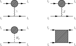
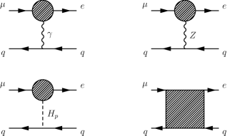
Figure 1: Generic one-loop diagrams contributing to LFV processes: 1) $l_{j}\to l_{i}\gamma$; 2) $l_{j}\to 3l_{i}$, mediated by $\gamma$ and $Z$ gauge bosons, by $H_{p}=h^{0},H^{0},A^{0}$ Higgs bosons and by boxes; 3) $\tau\to\mu\eta$ and $\tau\to e\eta$, mediated by $A^{0}$ Higgs boson and by $Z$ gauge boson; 4) $\mu-e$ conversion in nuclei, mediated by $\gamma$, and $Z$ gauge bosons, by $H_{p}=h^{0},H^{0}$ Higgs bosons, and by boxes.

The generic one-loop diagrams contributing to all the LFV processes above, are summarized in Fig.1. These include the $\gamma$-mediated diagrams, the $Z$-mediated diagrams, and the $h^{0}$, $H^{0}$ and $A^{0}$-mediated diagrams. The generic one-loop box diagrams are also shown in this figure. These also include the $\delta^{AB}_{ij}$’s but their sensitivities to these parameters are much lower than via the above quoted three-point vertices. They are, however, included in our analytical results and in our numerical evaluation.

For our forthcoming numerical analysis of these LFV processes we have implemented the full one-loop formulas into our private Fortran code. The analytical results are taken from various publications (with one of the authors as co-author): Ref. [15] for ${\rm BR}(l_{j}\to 3l_{i})$ and ${\rm BR}(l_{j}\to l_{i}\gamma)$, Ref. [18] for ${\rm BR}(\tau\to\mu\eta)$ and ${\rm BR}(\tau\to e\eta)$, and Ref. [17] for the $\mu-e$ conversion rate in heavy nuclei, relative to the muon capture rate ${\rm CR}(\mu-e,{\rm Nuclei})$. Following the same procedure of [18] we use Chiral Perturbation Theory for the needed hadronization of quark bilinears involved in the quark-level $\tau\to\mu qq^{\prime}$ and $\tau\to eqq^{\prime}$ decays that lead the $\eta$ particle in the final state. Our treatment of the heavy nuclei and the proper approximations to go from the LFV amplitudes at the parton level to the LFV rates at the nuclear level are described in [17]. For brevity, we omit to explicit here all these needed formulas for the computation of the LFV rates and refer the reader to the above quoted references for the details.

The list of specific one-loop diagrams contributing to the relevant $(l_{i}l_{j}\gamma)_{\rm 1-loop}$, $(l_{i}l_{j}Z)_{\rm 1-loop}$ $(l_{i}l_{j}h^{0})_{\rm 1-loop}$, $(l_{i}l_{j}H^{0})_{\rm 1-loop}$ and $(l_{i}l_{j}A^{0})_{\rm 1-loop}$ vertices can also be found in Refs. [15, 17]. The main contributions come from the loops with charginos/sneutrinos and with neutralinos/sleptons. This will be relevant for the analytical interpretation of our results below.

3.2 The MIA basic reference formulas

For completeness, and in order to get a better understanding of the forthcoming full one-loop results leading to the maximal allowed deltas and their behavior with the relevant MSSM parameters, we include in this section the main formulas for the LFV radiative decays within the Mass Insertion Approximation (MIA) that we take from Ref. [26]. These are simple formulas and illustrate clearly the qualitative behavior of the LFV rates with all the deltas and all the MSSM parameters. The branching ratios of the radiative $l_{j}\to l_{i}\gamma$ decays, with $ji=21$, $31$ and $32$, are:

$${\rm BR}(l_{j}\to l_{i}\gamma) = \frac{\alpha}{4}(\frac{m_{l_{j}}^{5}}{\Gamma_{l_{j}}})\left(|(A_{ij}^{L})|^{2}+|(A_{ij}^{R})|^{2}\right)$$ (11)

where $\Gamma_{l_{j}}$ is the total ${l_{j}}$ width, and the amplitudes, in the single delta insertion approximation, are given by [26]:

$$(A_{ij}^{L})_{\rm MIA} = \frac{\alpha_{2}}{4\pi}\Delta^{LL}_{ij}\left[\frac{f_{1n}(a_{L2})+f_{1c}(a_{L2})}{m_{\tilde{L}}^{4}}+\frac{\mu M_{2}\tan\beta}{(M_{2}^{2}-\mu^{2})}\frac{(f_{2n}(a_{L2},b_{L})+f_{2c}(a_{L2},b_{L}))}{m_{\tilde{L}}^{4}}\right]$$ (12)

$$+ \frac{\alpha_{1}}{4\pi}\Delta^{LL}_{ij}\left[\frac{f_{1n}(a_{L})}{m_{\tilde{L}}^{4}}+\mu M_{1}\tan\beta\left(\frac{-f_{2n}(a_{L},b_{L})}{m_{\tilde{L}}^{4}(M_{1}^{2}-\mu^{2})}+\frac{2f_{2n}(a_{L})}{m_{\tilde{L}}^{4}(m_{\tilde{R}}^{2}-m_{\tilde{L}}^{2})}\right)\right]$$

$$+ \frac{\alpha_{1}}{4\pi}\Delta^{LL}_{ij}\left[\frac{\mu M_{1}\tan\beta}{(m_{\tilde{R}}^{2}-m_{\tilde{L}}^{2})^{2}}\left(\frac{f_{3n}(a_{R})}{m_{\tilde{R}}^{2}}-\frac{f_{3n}(a_{L})}{m_{\tilde{L}}^{2}}\right)\right]$$

$$+ \frac{\alpha_{1}}{4\pi}\Delta^{LR}_{ij}\left[\frac{1}{(m_{\tilde{L}}^{2}-m_{\tilde{R}}^{2})}\left(\frac{M_{1}}{m_{l_{j}}}\right)\left(\frac{f_{3n}(a_{R})}{m_{\tilde{R}}^{2}}-\frac{f_{3n}(a_{L})}{m_{\tilde{L}}^{2}}\right)\right]$$

and

$$(A_{ij}^{R})_{\rm MIA} = \frac{\alpha_{1}}{4\pi}\Delta^{RR}_{ij}\left[\frac{4f_{1n}(a_{R})}{m_{\tilde{R}}^{4}}+\mu M_{1}\tan\beta\left(\frac{2f_{2n}(a_{R},b_{R})}{m_{\tilde{R}}^{4}(M_{1}^{2}-\mu^{2})}+\frac{2f_{2n}(a_{R})}{m_{\tilde{R}}^{4}(m_{\tilde{L}}^{2}-m_{\tilde{R}}^{2})}\right)\right]$$ (13)

$$+ \frac{\alpha_{1}}{4\pi}\Delta^{RR}_{ij}\left[\frac{\mu M_{1}\tan\beta}{(m_{\tilde{L}}^{2}-m_{\tilde{R}}^{2})^{2}}\left(\frac{f_{3n}(a_{L})}{m_{\tilde{L}}^{2}}-\frac{f_{3n}(a_{R})}{m_{\tilde{R}}^{2}}\right)\right]$$

$$+ \frac{\alpha_{1}}{4\pi}\Delta^{RL}_{ij}\left[\frac{1}{(m_{\tilde{R}}^{2}-m_{\tilde{L}}^{2})}\left(\frac{M_{1}}{m_{l_{j}}}\right)\left(\frac{f_{3n}(a_{L})}{m_{\tilde{L}}^{2}}-\frac{f_{3n}(a_{R})}{m_{\tilde{R}}^{2}}\right)\right]~{},$$

where $\alpha_{1}=(5/3)(\alpha/\cos^{2}\theta_{W})$, $\alpha_{2}=(\alpha/\sin^{2}\theta_{W})$, $a_{L2}=M_{2}^{2}/m_{\tilde{L}}^{2}$, $a_{L}=M_{1}^{2}/m_{\tilde{L}}^{2}$, $a_{R}=M_{1}^{2}/m_{\tilde{R}}^{2}$, $b_{L}=\mu^{2}/m_{\tilde{L}}^{2}$, $b_{R}=\mu^{2}/m_{\tilde{R}}^{2}$, $\Delta^{AB}_{ij}=\delta^{AB}_{ij}m_{\tilde{A}}m_{\tilde{B}}$ and $m_{\tilde{L}}$ and $m_{\tilde{R}}$ are the average slepton masses in the ${\tilde{L}}$ and ${\tilde{R}}$ slepton sectors, respectively. The $M_{1}$ and $M_{2}$ are the soft SUSY-breaking parameters in the U(1) and SU(2) gaugino sector, respectively. The $f_{in}$’s and $f_{ic}$’s are loop functions from neutralinos and charginos contributions, respectively, given by:

$$f_{1n}(a) = \frac{-17a^{3}+9a^{2}+9a-1+6a^{2}(a+3)\ln a}{24(1-a)^{5}}~{},$$

$$f_{2n}(a) = \frac{-5a^{2}+4a+1+2a(a+2)\ln a}{4(1-a)^{4}}~{},$$

$$f_{3n}(a) = \frac{1+2a\ln a-a^{2}}{2(1-a)^{3}}~{},$$

$$f_{1c}(a) = \frac{-a^{3}-9a^{2}+9a+1+6a(a+1)\ln a}{6(1-a)^{5}}~{},$$

$$f_{2c}(a) = \frac{-a^{2}-4a+5+2(2a+1)\ln a}{2(1-a)^{4}}~{},$$

$$f_{2n}(a,b) = f_{2n}(a)-f_{2n}(b)~{},$$

$$f_{2c}(a,b) = f_{2c}(a)-f_{2c}(b)~{}.$$ (14)

It is also very illustrative to compare the forthcoming results with those of the MIA for the case of equal mass scales, $m_{\tilde{L}}=m_{\tilde{R}}=\mu=M_{2}=M_{1}\equiv m_{S}$. From the previous formulas we get:

$$(A_{ij}^{L})_{\rm MIA} = \frac{\alpha_{2}}{4\pi}\delta^{LL}_{ij}\left[\frac{1}{240}\frac{1}{m_{S}^{2}}+\tan\beta\frac{1}{15}\frac{1}{m_{S}^{2}}\right]$$ (15)

$$+ \frac{\alpha_{1}}{4\pi}\delta^{LL}_{ij}\left[\frac{-1}{80}\frac{1}{m_{S}^{2}}+\tan\beta\frac{1}{12}\frac{1}{m_{S}^{2}}\right]$$

$$+ \frac{\alpha_{1}}{4\pi}\delta^{LR}_{ij}\left[\frac{1}{m_{S}m_{l_{j}}}\right]$$

and

$$(A_{ij}^{R})_{\rm MIA} = \frac{\alpha_{1}}{4\pi}\delta^{RR}_{ij}\left[\frac{-1}{20}\frac{1}{m_{S}^{2}}-\tan\beta\frac{1}{60}\frac{1}{m_{S}^{2}}\right]$$ (16)

$$+ \frac{\alpha_{1}}{4\pi}\delta^{RL}_{ij}\left[\frac{1}{m_{S}m_{l_{j}}}\right]~{}.$$

In all these basic MIA formulas one can see clearly the scaling of the BRs with all the deltas, in the single mass insertion approximation, and with the most relevant parameters for the present study, namely, the common/average SUSY mass $m_{S}$, and $\tan\beta$. These formulas will be used below in the interpretation of the full numerical results.

3.3 Experimental bounds on LFV

So far, LFV has not been observed. The best present (90% CL) experimental bounds on the previously selected LFV processes are summarized in the following:

$${\rm BR}(\mu\to e\gamma)<5.7\times 10^{-13}$$ [29]

$${\rm BR}(\tau\to\mu\gamma)<4.4\times 10^{-8}$$ [30]

$${\rm BR}(\tau\to e\gamma)<3.3\times 10^{-8}$$ [30]

$${\rm BR}(\mu\to eee)<1.0\times 10^{-12}$$ [32]

$${\rm BR}(\tau\to\mu\mu\mu)<2.1\times 10^{-8}$$ [33]

$${\rm BR}(\tau\to eee)<2.7\times 10^{-8}$$ [33]

$${\rm CR}(\mu-e,{\rm Au})<7.0\times 10^{-13}$$ [31]

$${\rm BR}(\tau\to\mu\eta)<2.3\times 10^{-8}$$ [34]

$${\rm BR}(\tau\to e\eta)<4.4\times 10^{-8}$$ [34] (17)

At present, the most constraining bounds are from ${\rm BR}(\mu\to e\gamma)$, which has been just improved by the MEG collaboration, and from ${\rm CR}(\mu-e,{\rm Au})$, both being at the ${\cal O}(10^{-13})$ level. Therefore, the 12 slepton mixings are by far the most constrained ones. All these nine upper bounds above will be applied next to extract the maximum allowed $|\delta^{AB}_{ij}|$ values.

3.4 MSSM scenarios

Regarding our choice of MSSM parameters for our forthcoming numerical analysis of the LFV processes, we have proceeded within two frameworks, both compatible with present data, that we describe in the following.

3.4.1 Framework 1

In the first framework, we have selected six specific points in the MSSM parameter space, $S1,...,S6$, as examples of points that are allowed by present data, including recent LHC searches and the measurements of the muon anomalous magnetic moment. In Tab. 1 the values of the various MSSM parameters as well as the values of the predicted MSSM mass spectra are summarized. They were evaluated with the program FeynHiggs [42]. For simplicity, and to reduce the number of independent MSSM input parameters we have assumed equal soft masses for the sleptons of the first and second generations (similarly for the squarks), equal soft masses for the left and right slepton sectors (similarly for the squarks, where $\tilde{Q}$ denotes the the “left-handed” squark sector, whereas $\tilde{U}$ and $\tilde{D}$ denote the up- and down-type parts of the “right-handed” squark sector) and also equal trilinear couplings for the stop, $A_{t}$, and sbottom squarks, $A_{b}$. In the slepton sector we just consider the stau trilinear coupling, $A_{\tau}$. The other trilinear sfermion couplings are set to zero value. Regarding the soft SUSY-breaking parameters for the gaugino masses, $M_{i}$ ($i=1,2,3$), we assume an approximate GUT relation. The pseudoscalar Higgs mass $M_{A}$, and the $\mu$ parameter are also taken as independent input parameters. In summary, the six points $S1,..,S6$ are defined in terms of the following subset of ten input MSSM parameters:

$$m_{\tilde{L}_{1}} = m_{\tilde{L}_{2}}\;;\;m_{\tilde{L}_{3}}\;(\mbox{with~{}}m_{\tilde{L}_{i}}=m_{\tilde{E}_{i}}\,\,,\,\,i=1,2,3)$$

$$m_{\tilde{Q}_{1}} = m_{\tilde{Q}_{2}}\;;\;m_{\tilde{Q}_{3}}\;(\mbox{with~{}}m_{\tilde{Q}_{i}}=m_{\tilde{U}_{i}}=m_{\tilde{D}_{i}}\,\,,\,\,i=1,2,3)$$

$$A_{t} = A_{b}\,\,;\,\,A_{\tau}$$

$$M_{2} = 2M_{1}\,=\,M_{3}/4\,\,;\,\,\mu$$

$$M_{A} \,\,;\,\, \tan\beta$$ (18)

	S1	S2	S3	S4	S5	S6
$m_{\tilde{L}_{1,2}}$	500	750	1000	800	500	1500
$m_{\tilde{L}_{3}}$	500	750	1000	500	500	1500
$M_{2}$	500	500	500	500	750	300
$A_{\tau}$	500	750	1000	500	0	1500
$\mu$	400	400	400	400	800	300
$\tan\beta$	20	30	50	40	10	40
$M_{A}$	500	1000	1000	1000	1000	1500
$m_{\tilde{Q}_{1,2}}$	2000	2000	2000	2000	2500	1500
$m_{\tilde{Q}_{3}}$	2000	2000	2000	500	2500	1500
$A_{t}$	2300	2300	2300	1000	2500	1500
$m_{\tilde{l}_{1}}-m_{\tilde{l}_{6}}$	489-515	738-765	984-1018	474-802	488-516	1494-1507
$m_{\tilde{\nu}_{1}}-m_{\tilde{\nu}_{3}}$	496	747	998	496-797	496	1499
$m_{{\tilde{\chi}}_{1}^{\pm}}-m_{{\tilde{\chi}}_{2}^{\pm}}$	375-531	376-530	377-530	377-530	710-844	247-363
$m_{{\tilde{\chi}}_{1}^{0}}-m_{{\tilde{\chi}}_{4}^{0}}$	244-531	245-531	245-530	245-530	373-844	145-363
$M_{h}$	126.6	127.0	127.3	123.1	123.8	125.1
$M_{H}$	500	1000	999	1001	1000	1499
$M_{A}$	500	1000	1000	1000	1000	1500
$M_{H^{\pm}}$	507	1003	1003	1005	1003	1502
$m_{\tilde{u}_{1}}-m_{\tilde{u}_{6}}$	1909-2100	1909-2100	1908-2100	336-2000	2423-2585	1423-1589
$m_{\tilde{d}_{1}}-m_{\tilde{d}_{6}}$	1997-2004	1994-2007	1990-2011	474-2001	2498-2503	1492-1509
$m_{\tilde{g}}$	2000	2000	2000	2000	3000	1200

Table 1: Selected points in the MSSM parameter space (upper part) and their corresponding spectra (lower part). All mass parameters and trilinear couplings are given in GeV.

The specific values of these ten MSSM parameters in Tab. 1, to be used in the forthcoming analysis of LFV, are chosen to provide different patterns in the various sparticle masses, but all leading to rather heavy spectra, thus they are naturally in agreement with the absence of SUSY signals at LHC. In particular all points lead to rather heavy squarks and gluinos above $1200\,\,\mathrm{GeV}$ and heavy sleptons above $500\,\,\mathrm{GeV}$ (where the LHC limits would also permit substantially lighter scalar leptons). The values of $M_{A}$ within the interval $(500,1500)\,\,\mathrm{GeV}$, $\tan\beta$ within the interval $(10,50)$ and a large $A_{t}$ within $(1000,2500)\,\,\mathrm{GeV}$ are fixed such that a light Higgs boson $h^{0}$ within the LHC-favoured range $(123,127)\,\,\mathrm{GeV}$ is obtained. It should also be noted that the large chosen values of $M_{A}\geq 500$ GeV place the Higgs sector of our scenarios in the so called decoupling regime[4], where the couplings of $h^{0}$ to gauge bosons and fermions are close to the SM Higgs couplings, and the heavy $H^{0}$ couples like the pseudoscalar $A^{0}$, and all heavy Higgs bosons are close in mass. Increasing $M_{A}$ the heavy Higgs bosons tend to decouple from low energy physics and the light $h^{0}$ behaves like $H_{\rm SM}$. This type of MSSM Higgs sector seems to be in good agreement with recent LHC data[37, 38]. We have checked with the code HiggsBounds [43] that the Higgs sector is in agreement with the LHC searches (where S3 is right “at the border”). Particularly, the so far absence of gluinos at LHC, forbids too low $M_{3}$ and, therefore, given the assumed GUT relation, forbids also a too low $M_{2}$. Consequently, the values of $M_{2}$ and $\mu$ are fixed as to get gaugino masses compatible with present LHC bounds. Finally, we have also required that all our points lead to a prediction of the anomalous magnetic moment of the muon in the MSSM that can fill the present discrepancy between the Standard Model prediction and the experimental value. Specifically, we use Refs. [39] and [44] to extract the size of this discrepancy, see also Ref. [45]:

$$(g-2)_{\mu}^{\rm exp}-(g-2)_{\mu}^{\rm SM}=(30.2\pm 9.0)\times 10^{-10}.$$ (19)

We then require that the SUSY contributions from charginos and neutralinos in the MSSM to one-loop level, $(g-2)_{\mu}^{\rm SUSY}$ be within the interval defined by $3\sigma$ around the central value in Eq. (19), namely:

$$(g-2)_{\mu}^{\rm SUSY}\in(3.2\times 10^{-10},57.2\times 10^{-10})$$ (20)

Our estimate of $(g-2)_{\mu}^{\rm SUSY}$ for the six $S1,..S6$ points with the code SPHENO [46] is (where FeynHiggs gives similar results), respectively,

$$(15.5\,(\mbox{S1}),\,13.8\,(\mbox{S2}),\,15.1\,(\mbox{S3}),16.7\,(\mbox{S4}),\,6.1\,(\mbox{S5}),\,7.9\,(\mbox{S6}))\,\times 10^{-10}$$ (21)

which are clearly within the previous allowed interval. The relatively low values are due to the relatively heavy slepton spectrum that was chosen. However, they are well within the preferred interval.

3.4.2 Framework 2

In the second framework, several possibilities for the MSSM parameters have been considered, leading to simple patterns of SUSY masses with specific relations among them and where the number of input parameters is strongly reduced. As in framework 1 the scenarios selected in framework 2 lead to predictions of $(g-2)_{\mu}$ and $M_{h}$ that are compatible with present data over a large part of the parameter space. To simplify the analysis of the upper bounds of the deltas, we will focus in scenarios where the mass scales that are relevant for the LFV processes are all set relative to one mass scale, generically called here $m_{\rm SUSY-EW}$. This implies setting the slepton soft masses, the gaugino soft masses, $M_{2}$ and $M_{1}$ and the $\mu$ parameter in terms of this $m_{\rm SUSY-EW}$. It should also be noted that these same mass parameters are the relevant ones for $(g-2)_{\mu}$. The remaining relevant parameter in both LFV and $(g-2)_{\mu}$ is $\tan\beta$, and the analysis below is performed in the ($m_{\rm SUSY-EW}$, $\tan\beta$) plane. Our selected LFV observables to be analized in framework 2 are the radiative $l_{j}\to l_{i}\gamma$ decays. As discussed before, these are expected to be the most constraining ones. On the other hand, since we are interested in choices of the MSSM parameters that lead to a prediction of $M_{h}$ that is compatible with LHC data, we also have to set the corresponding relevant mass parameters for this observable. These are mainly the squark soft masses and trilinear soft couplings, with particular relevance of those parameters of the third generation squarks. All these squark mass scales will be set, in our framework 2, relative to one single mass scale, $m_{\rm SUSY-QCD}$. Since we wish to explore a wide range in $\tan\beta$, from 5 to 60, $M_{A}$ is fixed to $1000\,\,\mathrm{GeV}$ to ensure the agreement with the present bounds in the $(\tan\beta,M_{A})$ plane from LHC searches [38]. Finally, to reduce even further the number of input parameters we will assume again an approximate GUT relation among the gaugino soft masses, $M_{2}=2M_{1}\,=\,M_{3}/4$ and the $\mu$ parameter will be set equal to $M_{2}$. Regarding the trilinear couplings, they will all be set to zero except those of the stop and sbottom sectors, being relevant for $M_{h}$, and that will be simplified to $A_{t}=A_{b}$. In summary, our scenarios in framework 2 are set in terms of four input parameters: $m_{\rm SUSY-EW}$, $m_{\rm SUSY-QCD}$, $M_{2}$ and $\tan\beta$. Generic scenarios in which the relevant parameters are fixed independently are called “phenomenological MSSM scenarios (pMSSM)” in the literature (see, for instance, [47, 48]). We refer to our scenarios here as “pMSSM-4”, indicating the number of free parameters. These kind of scenarios have the advantage of reducing considerably the number of input parameters respect to the MSSM and, consequently, making easier the analysis of their phenomenological implications.

For the forthcoming numerical analysis we consider the following specific pMSSM-4 mass patterns:

• $$m_{\tilde{L}} = m_{\tilde{E}}=m_{\rm SUSY-EW}$$

  $$M_{2} = m_{\rm SUSY-EW}$$

  $$m_{\tilde{Q}} = m_{\tilde{U}}=m_{\tilde{D}}=m_{\rm SUSY-QCD}$$

  $$A_{t} = 1.3\,m_{\rm SUSY-QCD}$$

  $$m_{\rm SUSY-QCD} = 2\,m_{\rm SUSY-EW}$$ (22)

• $$m_{\tilde{L}} = m_{\tilde{E}}=m_{\rm SUSY-EW}$$

  $$M_{2} = m_{\rm SUSY-EW}/5$$

  $$m_{\tilde{Q}} = m_{\tilde{U}}=m_{\tilde{D}}=m_{\rm SUSY-QCD}$$

  $$A_{t} = m_{\rm SUSY-QCD}$$

  $$m_{\rm SUSY-QCD} = 2\,m_{\rm SUSY-EW}$$ (23)

• $$m_{\tilde{L}} = m_{\tilde{E}}=m_{\rm SUSY-EW}$$

  $$M_{2} = 300\,\,{\rm GeV}$$

  $$m_{\tilde{Q}} = m_{\tilde{U}}=m_{\tilde{D}}=m_{\rm SUSY-QCD}$$

  $$A_{t} = m_{\rm SUSY-QCD}$$

  $$m_{\rm SUSY-QCD} = m_{\rm SUSY-EW}$$ (24)

• $$m_{\tilde{L}} = m_{\tilde{E}}=m_{\rm SUSY-EW}$$

  $$M_{2} = m_{\rm SUSY-EW}/3$$

  $$m_{\tilde{Q}} = m_{\tilde{U}}=m_{\tilde{D}}=m_{\rm SUSY-QCD}$$

  $$A_{t} = m_{\rm SUSY-QCD}$$

  $$m_{\rm SUSY-QCD} = m_{\rm SUSY-EW}$$ (25)

Where we have simplified the notation for the soft sfermion masses, by using $m_{\tilde{L}}$ for $m_{\tilde{L}}=m_{\tilde{L}_{1}}=m_{\tilde{L}_{2}}=m_{\tilde{L}_{3}}$, etc. In the forthcoming numerical analysis of the maximum allowed values of the deltas within these scenarios, the most relevant parameters $m_{\rm SUSY-EW}\equiv m_{\rm SUSY}$ and $\tan\beta$ will be varied within the intervals:

$$500\,\,{\rm GeV}\leq m_{\rm SUSY} \leq 2500\,\,{\rm GeV}$$

$$5\leq \tan\beta \leq 60$$ (26)

Due to the particular mass patterns chosen above, scenario (a) will deal with approximately equally heavy sleptons and charginos/neutralinos and with doubly heavy squarks; same for scenario (b) but with 1/5 lighter charginos/neutralinos; scenario (c) with equally heavy sleptons and squarks and charginos/neutralinos close to 300 GeV and scenario (d) with 1/3 lighter charginos/neutralinos. The values of $A_{t}$ have been selected to ensure that $M_{h}\sim 125-126\,\,\mathrm{GeV}$ over large parts of the ($m_{\rm SUSY}$, $\tan\beta$) plane.

3.5 Selected $\delta^{AB}_{ij}$ mixings

Finally, for our purpose in this paper, we need to select the slepton mixings and to set the range of values for the explored $\delta^{AB}_{ij}$’s. First, we work in a complete basis, that is we take into account the full set of twelve $\delta^{AB}_{ij}$’s. For simplicity, we will assume real values for these flavor slepton mixing parameters, therefore we will not have to be concerned with the Lepton Electric Dipole Moments (EDM). Concretely, the scanned interval in our estimates of LFV rates will be:

$$-1\leq\delta^{AB}_{ij}\leq+1$$ (27)

For each explored non-vanishing single delta, $\delta^{AB}_{ij}$, or pair of deltas, $(\delta^{AB}_{ij},\delta^{CD}_{kl})$, the corresponding slepton and sneutrino physical masses, the slepton and sneutrino rotation matrices, as well as the LFV rates will be numerically computed with our private Fortran code.

4 Results and discussion

4.1 Results in framework 1

The results of our numerical predictions of the branching ratios as functions of the single deltas $\delta^{AB}_{ij}$, for the various selected LFV processes and for the various scenarios S1 to S6 in framework 1, are collected in figures 2 through 10, where a comparison with the corresponding present upper experimental bound is also included, see Sect. 3.3. Figure 2 summarizes the status of $\delta^{LL}_{12}$, Fig. 3 that of $\delta^{LR}_{12}$, Fig. 4 that of $\delta^{RR}_{12}$. The analyzed experimental results are from ${\rm BR}(\mu\to e\gamma)$, ${\rm BR}(\mu\to 3e)$ and ${\rm CR}(\mu-e,\mbox{Nuclei})$. Figure 5 depicts the results of $\delta^{LL}_{13}$, Fig. 6 that of $\delta^{LR}_{13}$, Fig. 7 that of $\delta^{RR}_{13}$. The analyzed experimental results are from ${\rm BR}(\tau\to e\gamma)$, ${\rm BR}(\tau\to 3e)$ and ${\rm BR}(\tau\to e\eta)$. Figure 8 shows the results of $\delta^{LL}_{23}$, Fig. 9 that of $\delta^{LR}_{23}$, and Fig. 10 that of $\delta^{RR}_{23}$, where the experimental results are from ${\rm BR}(\tau\to\mu\gamma)$, ${\rm BR}(\tau\to 3\mu)$ and ${\rm BR}(\tau\to\mu\eta)$. The results for $\delta^{RL}_{ij}$ are indistinguishable from the corresponding ones for $\delta^{LR}_{ij}$, and consequently they have been omitted here.

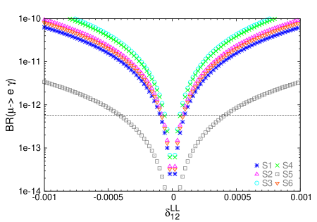
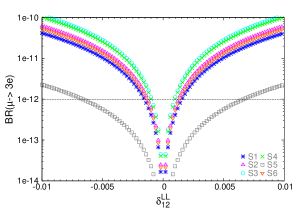
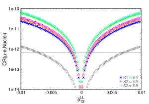
Figure 2: LFV rates for $\mu-e$ transitions as a function of slepton mixing $\delta_{12}^{LL}$.

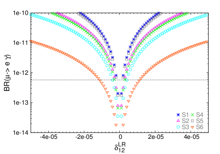
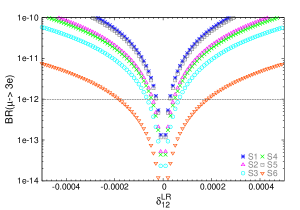
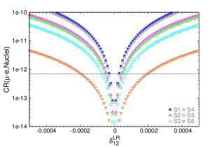
Figure 3: LFV rates for $\mu-e$ transitions as a function of slepton mixing $\delta_{12}^{LR}$. The corresponding plots for $\delta_{12}^{RL}$, not shown here, are indistinguishable from these.

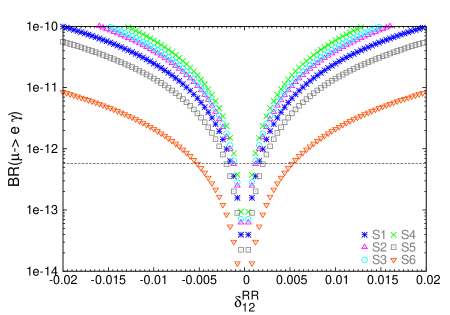
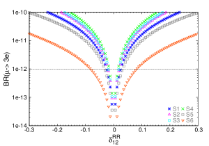
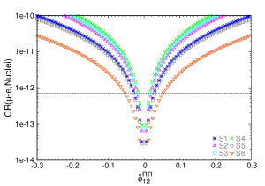
Figure 4: LFV rates for $\mu-e$ transitions as a function of slepton mixing $\delta_{12}^{RR}$.

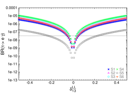
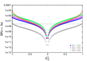
Figure 5: LFV rates for $\tau-e$ transitions as a function of slepton mixing $\delta_{13}^{LL}$

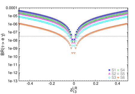
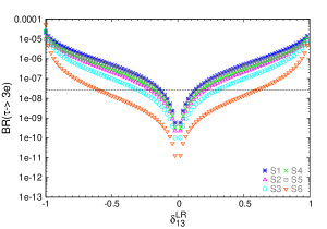
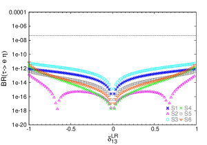
Figure 6: LFV rates for $\tau-e$ transitions as a function of slepton mixing $\delta_{13}^{LR}$. The corresponding plots for $\delta_{13}^{RL}$, not shown here, are indistinguishable from these.

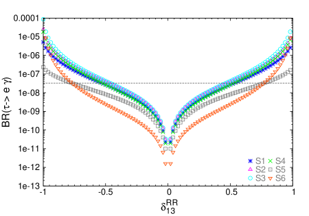
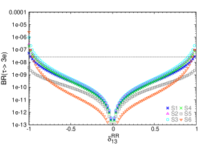
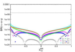
Figure 7: LFV rates for $\tau-e$ transitions as a function of slepton mixing $\delta_{13}^{RR}$.

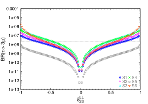
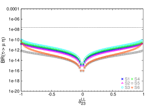
Figure 8: LFV rates for $\tau-\mu$ transitions as a function of slepton mixing $\delta_{23}^{LL}$.

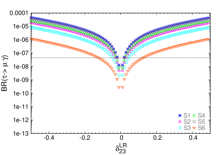
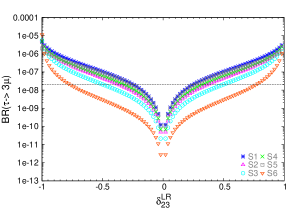
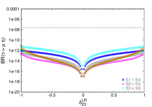
Figure 9: LFV rates for $\tau-\mu$ transitions as a function of slepton mixing $\delta_{23}^{LR}$. The corresponding plots for $\delta_{23}^{RL}$, not shown here, are indistinguishable from these.

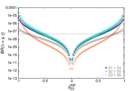
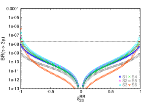
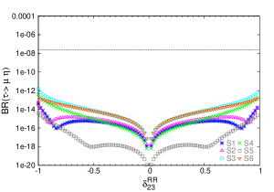
Figure 10: LFV rates for $\tau-\mu$ transitions as a function of slepton mixing $\delta_{23}^{RR}$.

A first look at these plots confirms the well known result that the most stringent bounds are for the mixings between the the first and the second slepton generations, 12. It is also evident that the bounds for the mixings between the second and the third slepton generations, 23, are similar to the bounds for the mixings between the first and the third generations, 13, and both are much weaker than the bounds on the 12-mixings. As another general result one can observe that, whereas all the 12-mixings are constrained by the three selected LFV processes, $\mu\to e\gamma$, $\mu\to 3e$ and $\mu-e$ conversion in heavy (Au) nuclei, the 23-mixings are not constrained, for the studied points, by the semileptonic tau decay $\tau\to\mu\eta$. Similarly, the 13-mixings are not constrained either, by $\tau\to e\eta$. The main reason for this is that the studied points S1-S6 all have very heavy $A^{0}$ Higgs bosons, $M_{A}=500-1500\,\,\mathrm{GeV}$ and therefore the decay channel mediated by this $A^{0}$ is much suppressed, even at large $\tan\beta$, where the contribution from $A^{0}$ to ${\rm BR}(\tau\to\mu\eta)$ and ${\rm BR}(\tau\to e\eta)$, which is the dominant one, grows as $(\tan\beta)^{6}$ [18, 19]. It should also be noted the appearance of two symmetric minima in ${\rm BR}(\tau\to\mu\eta)$ and ${\rm BR}(\tau\to e\eta)$ of figs 10 and 7 respectively, in the scenarios S5, S1 and S2. A similar feature can also be observed in ${\rm BR}(\tau\to e\eta)$ of fig 6 in scenario S2. For instance, in S5 these minima in ${\rm BR}(\tau\to e\eta)$ appear at $\delta_{13}^{RR}\sim\pm 0.5$. We have checked that the origin of these minima is due to the competing diagrams mediated by $A^{0}$ and $Z$ which give contributions of similar size for $\tan\beta\lesssim 30$ but with opposite sign , and this produces strong cancellations in the total rates. Similar comments apply to ${\rm BR}(\tau\to\mu\eta)$. Another general result, which confirms the known literature for particular models like SUSY-Seesaw models [15], is the evident correlation between the ${\rm BR}(l_{j}\to 3l_{i})$ and ${\rm BR}(l_{j}\to l_{i}\gamma)$ rates. It should be emphasized that we get these correlations in a model independent way and without the use of any approximation, like the mass insertion approximation or the large $\tan\beta$ approximation. Since our computation is full-one loop and has been performed in terms of physical masses, our findings are valid for any value of $\tan\beta$ and $\delta^{AB}_{ij}$’s. These correlations, confirmed in our plots, indicate that the general prediction guided by the photon-dominance behavior in ${\rm BR}(l_{j}\to 3l_{i})$ indeed works quite well for all the studied $\delta^{AB}_{ij}$’s and all the studied S1-S6 points. This dominance of the $\gamma$-mediated channel in the $l_{j}\to 3l_{i}$ decays allows to derive the following simplified relation:

$$\frac{{\rm BR}(l_{j}\to 3l_{i})}{{\rm BR}(l_{j}\to l_{i}\gamma)}=\frac{\alpha}{3\pi}\left(\log\frac{m_{l_{j}}^{2}}{m_{l_{i}}^{2}}-\frac{11}{4}\right)\,,$$ (28)

which gives the approximate values of $\frac{1}{440}$, $\frac{1}{94}$ and $\frac{1}{162}$ for $(l_{j}l_{i})=(\tau\mu),(\tau e)$ and $(\mu e)$, respectively. The ${\cal O}(\alpha)$ suppression in the predicted rates of ${\rm BR}(l_{j}\to 3l_{i})$ versus ${\rm BR}(l_{j}\to l_{i}\gamma)$ yields, despite the experimental sensitivities to the leptonic decays $l_{j}\to 3l_{i}$ have improved considerably in the last years, that the radiative decays $l_{j}\to l_{i}\gamma$ are still the most efficient decay channels in setting constraints to the slepton mixing parameters. This holds for all the intergenerational mixings, 12, 13 and 23. As discussed in [15], in the context of SUSY, there could be just a chance of departure from these ${\cal O}(\alpha)$ reduced ratios if the Higgs-mediated channels dominate the rates of the leptonic decays, but this does not happen in our S1-S6 scenarios, with rather heavy $H^{0}$ and $A^{0}$. We have checked that the contribution from these Higgs channels are very small and can be safely neglected, a scenario that is favored by the recent results from the heavy MSSM Higgs boson searches at the LHC [38].

This same behavior can be seen in the comparison between the ${\rm BR}(\mu\to e\gamma)$ and ${\rm CR}(\mu-e,{\rm Nuclei})$ rates. Again there is an obvious correlation in our plots for these two rates that can be explained by the same argument as above, namely, the photon-mediated contribution in $\mu-e$ conversion dominates the other contributions, for all the studied cases, and therefore the corresponding rates are suppressed by a ${\cal O}(\alpha)$ factor respect to the radiative decay rates. These correlations are clearly seen in all our plots for all the studied $\delta^{AB}_{ij}$’s and in all S1-S6 scenarios. The relevance of ${\rm CR}(\mu-e,{\rm Nuclei})$ as compared to ${\rm BR}(\mu\to 3e)$ is given by the fact that not only the present experimental bound is slightly better, but also that the future perspectives for the expected sensitivities are clearly more promising in the $\mu-e$ conversion case (see below). In general, as can be seen in our plots, the present bounds for $\delta^{AB}_{ij}$’s as obtained from ${\rm CR}(\mu-e,{\rm Nuclei})$ and ${\rm BR}(\mu\to 3e)$ are indeed very similar.

In summary, the best bounds that one can infer from our results in figures 2 through 10 come from the radiative $l_{j}\to l_{i}\gamma$ decays and we get the maximal allowed values for all $|\delta^{AB}_{ij}|$’s that are collected in Tab. 2 for each of the studied scenarios S1 to S6. They give an overall idea of the size of the bounds with respect to the latest experimental data. When comparing the results in this table for the various scenarios, we see that scenario S3 gives the most stringent constraints to the $\delta^{LL}_{ij}$ and $\delta^{RR}_{ij}$ mixings, in spite of having rather heavy sleptons with masses close to 1 TeV. The reason is well understood from the $\tan\beta$ dependence of the BRs which enhances the rates in the case of $LL$ and/or $RR$ single deltas at large $\tan\beta$, in agreement with the simple results of the MIA formulas in Eqs. (15) and (16). Here it should be noted that within S3 we have $\tan\beta=50$, which is the largest considered value in these S1-S6 scenarios. Something similar happens in S4 with $\tan\beta=40$. In contrast, the most stringent constraints on the $\delta^{LR}_{ij}$ mixings occur in scenarios S1 and S5. Here it is important to note that there are not enhancing $\tan\beta$ factors in the $\delta^{LR}_{ij}$ case. In fact, the contributions from the $\delta^{LR}_{ij}$’s to the most constraining LFV radiative decay rates are $\tan\beta$ independent, in agreement again with the MIA simple expectations (see Sect. 3.2). Consequently, the stringent constraints on $\delta^{LR}_{i,j}$ in S1 and S5 arise due to the relatively light sleptons in these scenarios.

	S1	S2	S3	S4	S5	S6
$|\delta^{LL}_{12}|_{\rm max}$	$10\times 10^{-5}$	$7.5\times 10^{-5}$	$5\times 10^{-5}$	$6\times 10^{-5}$	$42\times 10^{-5}$	$8\times 10^{-5}$
$|\delta^{LR}_{12}|_{\rm max}$	$2\times 10^{-6}$	$3\times 10^{-6}$	$4\times 10^{-6}$	$3\times 10^{-6}$	$2\times 10^{-6}$	$1.2\times 10^{-5}$
$|\delta^{RR}_{12}|_{\rm max}$	$1.5\times 10^{-3}$	$1.2\times 10^{-3}$	$1.1\times 10^{-3}$	$1\times 10^{-3}$	$2\times 10^{-3}$	$5.2\times 10^{-3}$
$|\delta^{LL}_{13}|_{\rm max}$	$5\times 10^{-2}$	$5\times 10^{-2}$	$3\times 10^{-2}$	$3\times 10^{-2}$	$23\times 10^{-2}$	$5\times 10^{-2}$
$|\delta^{LR}_{13}|_{\rm max}$	$2\times 10^{-2}$	$3\times 10^{-2}$	$4\times 10^{-2}$	$2.5\times 10^{-2}$	$2\times 10^{-2}$	$11\times 10^{-2}$
$|\delta^{RR}_{13}|_{\rm max}$	$5.4\times 10^{-1}$	$5\times 10^{-1}$	$4.8\times 10^{-1}$	$5.3\times 10^{-1}$	$7.7\times 10^{-1}$	$7.7\times 10^{-1}$
$|\delta^{LL}_{23}|_{\rm max}$	$6\times 10^{-2}$	$6\times 10^{-2}$	$4\times 10^{-2}$	$4\times 10^{-2}$	$27\times 10^{-2}$	$6\times 10^{-2}$
$|\delta^{LR}_{23}|_{\rm max}$	$2\times 10^{-2}$	$3\times 10^{-2}$	$4\times 10^{-2}$	$3\times 10^{-2}$	$2\times 10^{-2}$	$12\times 10^{-2}$
$|\delta^{RR}_{23}|_{\rm max}$	$5.7\times 10^{-1}$	$5.2\times 10^{-1}$	$5\times 10^{-1}$	$5.6\times 10^{-1}$	$8.3\times 10^{-1}$	$8\times 10^{-1}$

Table 2: Present upper bounds on the slepton mixing parameters $|\delta^{AB}_{ij}|$ for the selected S1-S6 MSSM points defined in Tab. 1. The bounds for $|\delta^{RL}_{ij}|$ are similar to those of $|\delta^{LR}_{ij}|$.

So far, we have studied the case where just one mixing delta is allowed to be non-vanishing. However, it is known in the literature[25, 26] that one can get more stringent or more lose bounds in some particular cases if, instead, two (or even more) deltas are allowed to be non-vanishing. In order to study the implications of these scenarios with two deltas, we have analyzed the improved bounds on pairs of mixings of the 13 and 23 type which are at present the less constrained as long each delta is analyzed singly.

First we have looked into the various delta pairings of 23 type, $(\delta^{AB}_{23},\delta^{CD}_{23})$, and we have found that some of them lead to interesting interferences in the ${\rm BR}(\tau\to\mu\gamma)$ rates that can be either constructive or destructive, depending on the relative delta signs, therefore leading to either a reduction or an enhancement, respectively, in the maximum allowed delta values as compared to the one single delta case. More specifically, we have found interferences in ${\rm BR}(\tau\to\mu\gamma)$ for the case of non-vanishing $(\delta^{LR}_{23},\delta^{LL}_{23})$ pairs that are constructive if these deltas are of equal sign, and destructive if they are of opposite sign. Similarly, we have also found interferences in ${\rm BR}(\tau\to\mu\gamma)$ for the case of non-vanishing $(\delta^{RL}_{23},\delta^{RR}_{23})$ pairs that are constructive if they are of equal sign, and destructive if they are of opposite sign. However, in this latter case the size of the interference is very small and does not lead to very relevant changes with respect to the single delta case. The numerical results for the most interesting case of $(\delta^{LR}_{23},\delta^{LL}_{23})$ are shown in Fig. 11. We have analyzed the six previous points, S1 through S6, and a new point S7 with extremely heavy sleptons and whose relevant parameters for this analysis of the 23 delta bounds are as follows:

$$S7 : m_{\tilde{L}_{1,2,3}}=m_{\tilde{E}_{1,2,3}}=10000\,\,{\rm GeV}$$ (29)

$$\mu=2000\,\,{\rm GeV};\tan\beta=60$$

$$M_{2}=2000\,\,{\rm GeV};M_{1}=1000\,\,{\rm GeV}$$

This figure exemplifies in a clear way that for some of the studied scenarios the destructive interferences can be indeed quite relevant and produce new areas in the $(\delta^{LR}_{23},\delta^{LL}_{23})$ plane with relatively large allowed values of both $|\delta^{LR}_{23}|$ and $|\delta^{LL}_{23}|$ mixings. For instance, the orange contour which corresponds to the maximum allowed values for scenario S6, leads to allowed mixings as large as $(\delta^{LR}_{23},\delta^{LL}_{23})\sim(\pm 0.6,\mp 0.6)$. We also learn from this plot, that the relevance of this $\delta^{LR}_{23}-\delta^{LL}_{23}$ interference grows in the following order: Scenario S5 (grey contour) that has the smallest interference effect, then S1, S2, S4, S3 and S6 that has the largest interference effect. This growing interference effect is seen in the plot as the contour being rotated anti-clockwise from the most vertical one (S1) to the most inclined one (S6). Furthermore, the size of the parameter space bounded by these contours also grows, implying that “more” parameter combinations are available for these two deltas. It should be noted that, whereas the existence of the interference effect can be already expected from the simple MIA formulas of Eqs. (15) and (16), the final found shape of these contours in fig.11 and their quantitative relevance cannot be explained by these simple formulas. The separation from the MIA expectations are even larger in the new studied scenario S7, as can be clearly seen in this figure. The big black contour, centered at zero, contains a rather large allowed area in the $(\delta^{LR}_{23},\delta^{LL}_{23})$ plane, allowing values, for instance, of $(\delta^{LR}_{23},\delta^{LL}_{23})\sim(\pm 0.5,\mp 0.5)$. Furthermore, in this S7 there appear new allowed regions at the upper left and lower right corners of the plot with extreme allowed values as large as $(\pm 0.9,\mp 0.9)$. These “extreme” solutions are only captured by a full one-loop calculation and cannot be explained by the simple MIA formulas.

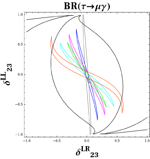
Figure 11: Maximum allowed values of $(\delta^{LR}_{23},\delta^{LL}_{23})$ in the scenarios S1 (dark blue), S2 (magenta), S3 (light blue), S4 (green), S5 (grey), S6 (orange) and S7 (black). The contourlines shown correspond to the present experimental upper limit: ${\rm BR}(\tau\to\mu\gamma)_{\rm max}=4.4\times 10^{-8}$. For each scenario the allowed deltas are those inside the corresponding contourline.

We now turn to examples in which more stringent bounds on combinations of two deltas are derived. In particular, we have explored the restrictions that are obtained on the (13,23) mixing pairs from the present bounds on ${\rm BR}(\mu\to e\gamma)$ and ${\rm CR}(\mu-e,{\rm nuclei})$. In figures 12 and 13 we show the results of this analysis for the S1 point. We have only selected the pairs where we have found improved bounds respect to the previous single delta analysis. From Fig. 12 we conclude that, for S1, the maximal allowed values by present $\mu\to e\gamma$ (($\mu-e$ conversion)) searches are (given specifically here for equal input deltas):

$$(|\delta^{LL}_{23}|_{\rm max},|\delta^{RL}_{13}|_{\rm max}) = (0.0015,0.0015)\,\,((0.0062,0.0062))\,\,$$ (30)

These numbers can be understood as follows: if, for instance, $\delta^{RL}_{13}=0.0015$ then $|\delta^{LL}_{23}|<0.0015$. If, on the other hand, one delta goes to zero the bound on the other delta disappears (from this particular observable). We find equal bounds as in Eq. (30) for: $(|\delta^{RL}_{23}|_{\rm max},|\delta^{LL}_{13}|_{\rm max})$, $(|\delta^{LR}_{23}|_{\rm max},|\delta^{RR}_{13}|_{\rm max})$ and $(|\delta^{RR}_{23}|_{\rm max},|\delta^{LR}_{13}|_{\rm max})$.

Other pairings of deltas give less stringent bounds than Eq. (30) but still more stringent than the ones from the single delta analysis. In particular, we get:

$$(|\delta^{LL}_{23}|_{\rm max},|\delta^{RR}_{13}|_{\rm max}) = (0.0073,0.0073)\,\,((0.031,0.031))\,\,$$ (31)

And we get equal bounds as in Eq. (31) for: $(|\delta^{RR}_{23}|_{\rm max},|\delta^{LL}_{13}|_{\rm max})$, $(|\delta^{LR}_{23}|_{\rm max},|\delta^{RL}_{13}|_{\rm max})$ and $(|\delta^{RL}_{23}|_{\rm max},|\delta^{LR}_{13}|_{\rm max})$.

Finally, from Fig. 13 we get:

$$(|\delta^{LL}_{23}|_{\rm max},|\delta^{LL}_{13}|_{\rm max}) = (0.013,0.013)\,\,((0.056,0.056))\,\,$$ (32)

and

$$(|\delta^{RR}_{23}|_{\rm max},|\delta^{RR}_{13}|_{\rm max}) = (0.036,0.036)\,\,((0.16,0.16))\,\,$$ (33)

We have also studied the implications of the future expected sensitivities in both ${\rm BR}(\mu\to e\gamma)<10^{-14}$ [49] and ${\rm CR}(\mu-e,{\rm Nuclei})<2.6\times 10^{-17}$ [50], which are anticipated from future searches. From our results in Figs. 12 and 13 we conclude that the previous bounds in Eqs. (30), (31), (32) and (33) will be improved (for both $\mu\to e\gamma$ and $\mu-e$ conversion) to $(0.0005,0.0005)$, $(0.0025,0.0025)$, $(0.005,0.005)$ and $(0.01,0.01)$, respectively.

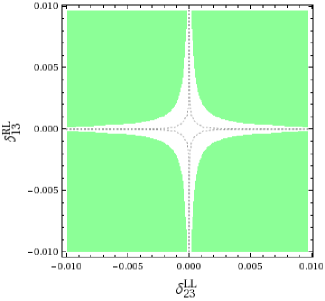
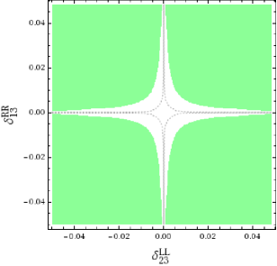
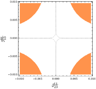
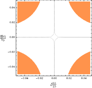
Figure 12: Bounds on pairs of slepton mixing parameters of (23,13) type for scenario S1: a) ($\delta_{23}^{LL}$,$\delta_{13}^{RL}$) in first column. Identical plots, not shown here, are found for: ($\delta_{23}^{RL}$,$\delta_{13}^{LL}$), ($\delta_{23}^{LR}$,$\delta_{13}^{RR}$), and ($\delta_{23}^{RR}$,$\delta_{13}^{LR}$); b) ($\delta_{23}^{LL}$,$\delta_{13}^{RR}$) in second column. Identical plots, not shown here, are found for: ($\delta_{23}^{RR}$,$\delta_{13}^{LL}$), ($\delta_{23}^{LR}$,$\delta_{13}^{RL}$), and ($\delta_{23}^{RL}$,$\delta_{13}^{LR}$). First row: Shaded regions (in green) are disallowed by the present upper experimental limit on ${\rm BR}(\mu\to e\gamma)$. Second row: Shaded regions (in orange) are disallowed by the present upper experimental limit on ${\rm CR}(\mu-e,{\rm Nuclei})$. The allowed central areas in white will be shrinked by the future expected sensitivities in both $\mu\to e\gamma$ and $\mu-e$ conversion experimental searches (see text) to the small areas around the origin delimited by the dotted lines.

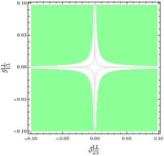
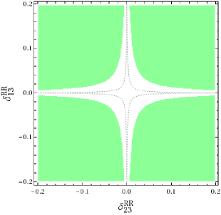
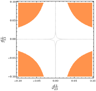
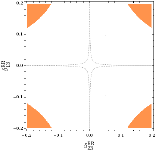
Figure 13: Bounds on pairs of slepton mixing parameters of (23,13) type for scenario S1: a) ($\delta_{23}^{LL}$,$\delta_{13}^{LL}$) in first column; b) ($\delta_{23}^{RR}$,$\delta_{13}^{RR}$) in second column. First row: Shaded regions (in green) are disallowed by ${\rm BR}(\mu\to e\gamma)$. Second row: Shaded regions (in orange) are disallowed by ${\rm CR}(\mu-e,{\rm Nuclei})$. All inputs and explanations are as in Fig. 12.

4.2 Results in framework 2

The main goal of this part is to investigate how the upper bounds for the slepton mixing deltas that we have found previously could change for different ranges of the MSSM parameter space, that go beyond the selected S1-S6 points.

In order to explore the variation of these bounds for different choices in the MSSM parameter space, we investigate the four qualitatively different pMSSM-4 scenarios (a), (b), (c) and (d) defined in Eqs. (22), (23), (24) and (25), respectively. As explained above, the idea is to explore generic scenarios that are compatible with present data, in particular with the measurement of a Higgs boson mass, which we interpret as the mass of the light ${\cal CP}$-even Higgs boson in the MSSM, and the present experimental measurement of $(g-2)_{\mu}$. Taking these experimental results into account, we have re-analyzed the full set of bounds for the single deltas that are extracted from the most restrictive LFV processes as a function of the two most relevant parameters in our framework 2: the generic SUSY mass scale $m_{\rm SUSY}$ $(\equiv m_{\rm SUSY-EW})$ and $\tan\beta$. In order to find $M_{h}$ around $\sim 125-126\,\,\mathrm{GeV}$ the scale $m_{\rm SUSY-QCD}$ as well as the trilinear couplings have been chosen to sufficiently high values, see Sect. 3.4.2. For the analysis in this framework 2, we use the bounds on the radiative decays, $l_{j}\to l_{i}\gamma$ which, as we have already shown, are at present the most restrictive ones in the case of one single non-vanishing delta. And to simplify the analysis in this part of the work, we use the mass insertion approximation (MIA) formulas of Eqs. (11) through (14) to evaluate the ${\rm BR}(l_{j}\to l_{i}\gamma)$ rates. We have checked that these simple MIA formulas provide a sufficiently accurate estimate of the LFV rates in the case of single deltas, in agreement with Ref. [26].

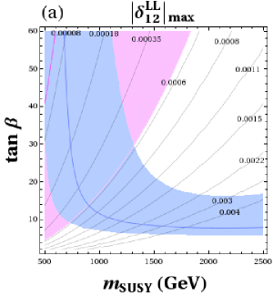
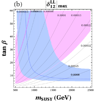
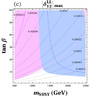
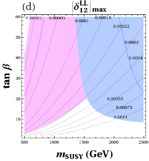
Figure 14: Contourlines in the ($m_{\rm SUSY}$, $\tan\beta$) plane of maximum slepton mixing $|\delta_{12}^{LL}|_{\rm max}$ that are allowed by LFV searches in $\mu\to e\gamma$ for scenarios (a), (b), (c) and (d) of our framework 2, defined in section 3.4.2. The shaded areas in pink are the regions leading to a $(g-2)_{\mu}^{\rm SUSY}$ prediction in the $(3.2,57.2)\times 10^{-10}$ interval. The interior pink contourline (without number) corresponds to setting $(g-2)_{\mu}^{\rm SUSY}$ exactly at the central value of the discrepancy $(g-2)_{\mu}^{\rm exp}-(g-2)_{\mu}^{\rm SM}=30.2\times 10^{-10}$ . The shaded overimposed areas in blue are the regions leading to a $M_{h}$ prediction within the $(123,127)\,\,\mathrm{GeV}$ interval. The interior blue contourline (without number) corresponds to the particular $M_{h}=125\,\,\mathrm{GeV}$ value.

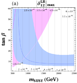
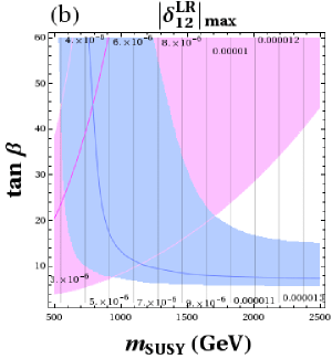
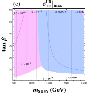
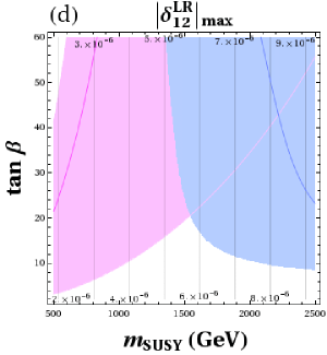
Figure 15: Contourlines in the ($m_{\rm SUSY}$, $\tan\beta$) plane of maximum slepton mixing $|\delta_{12}^{LR}|_{\rm max}$ that are allowed by LFV searches in $\mu\to e\gamma$. All inputs and explanations are as in Fig. 14.

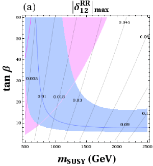
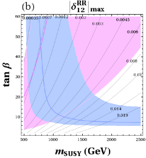
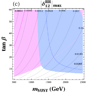
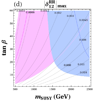
Figure 16: Contourlines in the ($m_{\rm SUSY}$, $\tan\beta$) plane of maximum slepton mixing $|\delta_{12}^{RR}|_{\rm max}$ that are allowed by LFV searches in $\mu\to e\gamma$. All inputs and explanations are as in Fig. 14.

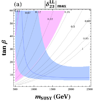
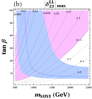
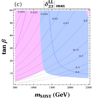
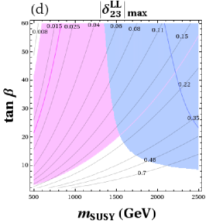
Figure 17: Contourlines in the ($m_{\rm SUSY}$, $\tan\beta$) plane of maximum slepton mixing $|\delta_{23}^{LL}|_{\rm max}$ that are allowed by LFV searches in $\tau\to\mu\gamma$. All inputs and explanations are as in Fig. 14. Similar results/plots (not shown) are obtained for contourlines of maximum slepton mixing $|\delta_{13}^{LL}|_{\rm max}$ that are allowed by LFV searches in $\tau\to e\gamma$.

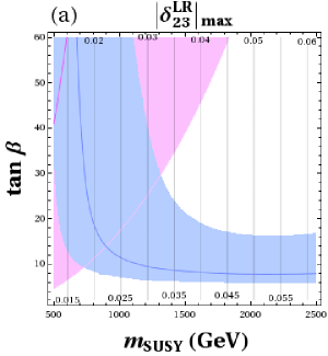
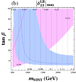
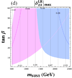
Figure 18: Contourlines in the ($m_{\rm SUSY}$, $\tan\beta$) plane of maximum slepton mixing $|\delta_{23}^{LR}|_{\rm max}$ that are allowed by LFV searches in $\tau\to\mu\gamma$. All inputs and explanations are as in Fig. 14. Similar results/plots (not shown) are obtained for contourlines of maximum slepton mixing $|\delta_{13}^{LR}|_{\rm max}$ that are allowed by LFV searches in $\tau\to e\gamma$.

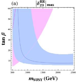
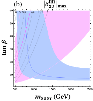
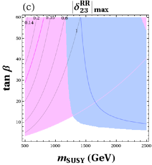
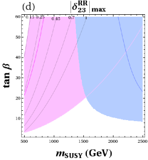
Figure 19: Contourlines in the ($m_{\rm SUSY}$, $\tan\beta$) plane of maximum slepton mixing $|\delta_{23}^{RR}|_{\rm max}$ that are allowed by LFV searches in $\tau\to\mu\gamma$. All inputs and explanations are as in Fig. 14. Notice that only contourlines with $|\delta_{23}^{RR}|_{\rm max}\leq 1$ are included. In the scenario (a) the countourlines with $|\delta_{23}^{RR}|_{\rm max}\leq 1$ are out of the region in the parameter space shown in this figure. Similar results/plots (not shown) are obtained for contourlines of maximum slepton mixing $|\delta_{13}^{RR}|_{\rm max}$ that are allowed by LFV searches in $\tau\to e\gamma$.

We present the numerical results of our analysis in framework 2 that are shown in Figs. 14 through 19. Figures 14, 15 and 16 show the bounds for the slepton mixing of 12-type as extracted from present $\mu\to e\gamma$ searches. Figures 17, 18 and 19 show the bounds for the slepton mixing of 23-type as extracted from present $\tau\to\mu\gamma$ searches. It should be noted that the bounds for the slepton mixings of 13-type (not shown here) are equal (in the MIA) to those of 23-type. In each plot we show the resulting contourlines in the ($m_{\rm SUSY}$, $\tan\beta$) plane of maximum allowed slepton mixing. In addition we also show in each plot the areas in the pMSSM-4 parameter space for that particular scenario that lead to values of the lightest Higgs boson mass compatible with LHC data, and at the same time to predictions of the muon anomalous magnetic moment also compatible with data. As in the previous framework 1, we use here again FeynHiggs [42] to evaluate $M_{h}$ and SPHENO [46] to evaluate $(g-2)_{\mu}$ (where FeynHiggs gives very similar results). The shaded areas in pink are the regions leading to a $(g-2)_{\mu}^{\rm SUSY}$ prediction, from the SUSY one-loop contributions, in the allowed by data $(3.2,57.2)\times 10^{-10}$ interval. The interior pink contourline corresponds to setting $(g-2)_{\mu}^{\rm SUSY}$ exactly at the central value of the discrepancy $(g-2)_{\mu}^{\rm exp}-(g-2)_{\mu}^{\rm SM}=30.2\times 10^{-10}$. The shaded overimposed areas in blue are the regions leading to a $M_{h}$ prediction within the $(123,127)\,\,\mathrm{GeV}$ interval. The interior blue contourline corresponds to the particular $M_{h}=125\,\,\mathrm{GeV}$ value.

From these plots in the ($m_{\rm SUSY}$, $\tan\beta$) plane one can draw the following conclusions:

• For each scenario (a), (b), (c) and (d) one can derive the corresponding upper bound for each $|\delta^{AB}_{ij}|$ at a given ($m_{\rm SUSY}$, $\tan\beta$) point in this plane.

• The maximal allowed values of the $\delta^{LL}_{ij}$’s and $\delta^{RR}_{ij}$’s scale with $m_{\rm SUSY}$ and $\tan\beta$ approximately as expected, growing with increasing $m_{\rm SUSY}$ as $\sim m_{\rm SUSY}^{2}$ and decreasing with increasing (large) $\tan\beta$ as $\sim 1/\tan\beta$. The maximal allowed values of the $\delta^{LR}_{ij}$’s (and similarly $\delta^{RL}_{ij}$’s) are independent on $\tan\beta$ and grow approximately as $\sim m_{\rm SUSY}$ with increasing $m_{\rm SUSY}$. This is in agreement with the qualitative behavior found in the approximation formulas, Eqs. (15) and (16) of the MIA results in the simplest case of only one mass scale, $m_{S}$.

• The intersections between the allowed areas by the required $(g-2)_{\mu}$ and $M_{h}$ intervals move from the left side, $m_{\rm SUSY}\sim 500-1300\,\,\mathrm{GeV}$ to the right side of the plots, $m_{\rm SUSY}\sim 1300-2500\,\,\mathrm{GeV}$ from scenarios (a) through (d). This is clearly the consequence of the fact that $(g-2)_{\mu}$ requires a rather light SUSY-EW sector, i.e. light charginos, neutralinos and sleptons, and a rather large $\tan\beta$, and that $M_{h}$ requires a rather heavy SUSY squark sector. Here we are using a common reference SUSY scale $m_{\rm SUSY}$, relating all the SUSY sparticle masses, both in the SUSY-EW and SUSY-QCD sectors, leading to this “tension”. (A more lose connection between these two sectors would yield a more relaxed combination of the $(g-2)_{\mu}$ and $M_{h}$ experimental results.) In fact, in our plots one can observe that the particular contourlines for the “prefered” values of $(g-2)_{\mu}$ and $M_{h}$ by data (i.e. the interior blue and pink contourlines) only cross in scenario (b) at $m_{\rm SUSY}$ around $800\,\,\mathrm{GeV}$ and $\tan\beta\sim 45$ and get close, although not crossing, in scenario (a) at $m_{\rm SUSY}\sim 650\,\,\mathrm{GeV}$ and very large $\tan\beta\sim 60$. However, taking the uncertainties into account the overlap regions are quite substantial.

• By assuming a favored region in the ($m_{\rm SUSY}$,$\tan\beta$) parameter space given by the intersect of the two $(g-2)_{\mu}$ (in pink) and $M_{h}$ (in blue) areas, one can extract improved bounds for the slepton mixing deltas valid in these intersects. Those bounds give a rough idea of which parameter regions in the pMSSM-4 are in better agreement with the experimental data on $(g-2)_{\mu}$ and $M_{h}$. The following intervals for the maximum allowed $|\delta^{AB}_{ij}|$ values can be deduced from our plots in these intersecting regions:

  Scenario (a):

  $|\delta^{LL}_{12}|_{\rm max}\sim(6,60)\times 10^{-5}$

  $|\delta^{LR}_{12}|_{\rm max}\sim(1.2,3.2)\times 10^{-6}$

  $|\delta^{RR}_{12}|_{\rm max}\sim(3,25)\times 10^{-3}$

  $|\delta^{LL}_{23}|_{\rm max}\sim(3,35)\times 10^{-2}$

  $|\delta^{LR}_{23}|_{\rm max}\sim(1,3.2)\times 10^{-2}$

  $|\delta^{RR}_{23}|_{\rm max}\sim(10)\times 10^{-1}$

  Scenario (b):

  $|\delta^{LL}_{12}|_{\rm max}\sim(1.5,27)\times 10^{-5}$

  $|\delta^{LR}_{12}|_{\rm max}\sim(3,9.2)\times 10^{-6}$

  $|\delta^{RR}_{12}|_{\rm max}\sim(0.35,7)\times 10^{-3}$

  $|\delta^{LL}_{23}|_{\rm max}\sim(0.7,15)\times 10^{-2}$

  $|\delta^{LR}_{23}|_{\rm max}\sim(3,9.5)\times 10^{-2}$

  $|\delta^{RR}_{23}|_{\rm max}\sim(2,10)\times 10^{-1}$

  Scenario (c):

  $|\delta^{LL}_{12}|_{\rm max}\sim(5,22)\times 10^{-5}$

  $|\delta^{LR}_{12}|_{\rm max}\sim(5,22)\times 10^{-6}$

  $|\delta^{RR}_{12}|_{\rm max}\sim(1.2,10)\times 10^{-3}$

  $|\delta^{LL}_{23}|_{\rm max}\sim(3,15)\times 10^{-2}$

  $|\delta^{LR}_{23}|_{\rm max}\sim(5,22)\times 10^{-2}$

  $|\delta^{RR}_{23}|_{\rm max}\sim(6,10)\times 10^{-1}$

  Scenario (d):

  $|\delta^{LL}_{12}|_{\rm max}\sim(10,30)\times 10^{-5}$

  $|\delta^{LR}_{12}|_{\rm max}\sim(5,9)\times 10^{-6}$

  $|\delta^{RR}_{12}|_{\rm max}\sim(1.2,4)\times 10^{-3}$

  $|\delta^{LL}_{23}|_{\rm max}\sim(5,20)\times 10^{-2}$

  $|\delta^{LR}_{23}|_{\rm max}\sim(5,9.5)\times 10^{-2}$

  $|\delta^{RR}_{23}|_{\rm max}\sim(7,10)\times 10^{-1}$

It should be noted that in the previous upper bounds, the particular $10\times 10^{-1}$ value appearing in $|\delta^{RR}_{23}|_{\rm max}$ really means 1 or larger that 1, since we have not explored out of the $-1\leq\delta^{AB}_{ij}\leq 1$ intervals. Particularly, in scenario (a) which has the heaviest gauginos, we find that all values in the $-1\leq\delta^{RR}_{23}\leq 1$ interval are allowed by LFV data.

Finally, one can shortly summarize the previous $|\delta^{AB}_{ij}|_{\rm max}$ intervals found from LFV searches, by just signaling the typical intervals for each delta, in the favored by LHC and $(g-2)_{\mu}$ data MSSM parameter space region, where the predictions in all scenarios lay at: $|\delta^{LL}_{12}|_{\rm max}\sim{\cal O}(10^{-5},10^{-4})$, $|\delta^{LR}_{12}|_{\rm max}\sim{\cal O}(10^{-6},10^{-5})$, $|\delta^{RR}_{12}|_{\rm max}\sim{\cal O}(10^{-3},10^{-2})$, $|\delta^{LL}_{23}|_{\rm max}\sim{\cal O}(10^{-2},10^{-1})$, $|\delta^{LR}_{23}|_{\rm max}\sim{\cal O}(10^{-2},10^{-1})$, $|\delta^{RR}_{23}|_{\rm max}\sim{\cal O}(10^{-1},10^{0})$. Very similar general bounds as for the 23 mixing are found for the 13 mixing.

5 Conclusions

We presented an up-to-date comparison of the most recent experimental limits on LFV observables and their predictions within the MSSM. The LFV observables include ${\rm BR}(\mu\to e\gamma)$ (in particular including the latest MEG results), ${\rm BR}(\tau\to\mu\gamma)$, ${\rm BR}(\tau\to e\gamma)$, ${\rm BR}(\mu\to 3e)$, ${\rm BR}(\tau\to 3\mu)$, ${\rm BR}(\tau\to 3e)$, ${\rm BR}(\tau\to\mu\eta)$, ${\rm BR}(\tau\to e\eta)$ and ${\rm CR}(\mu-e,{\rm nuclei})$. Within the MSSM the calculations were performed at the full one-loop level with the full (s)lepton flavor structure, i.e. not relying on the mass insertion or other approximations. The results have been combined into a Fortran code allowing for a fast joint evaluation. For convenience we also summarized the relevant approximation formulas which have been shown to be valid for not too large values of the LFV parameters, which are given as $\delta_{ij}^{AB}$ with $A,B=L,R$ and $i,j=1,2,3$.

In the first part we analyzed six representative scenarios which are in agreement with current bounds on the SUSY and Higgs searches at the LHC. We derived the most up-to-date bounds on $\delta_{ij}^{AB}$ within these six scenarios, thus giving an idea of the overall size of these parameters taking the latest experimental bounds into account. As shown in previous analyses, the observables ${\rm BR}(l_{i}\to l_{j}\gamma)$ continue to give the most stringent constraints on $\delta_{ij}^{AB}$ for all $A,B=L,R$. Apart from bounds on single $\delta_{ij}^{AB}$’s we also derived bounds on two parameters simultaneously, and studied where either a positive or a negative interference of the two $\delta$’s can be observed. As a prime example, in the case of mixings of 23 type, we found that due to a negative interference, values of $|\delta_{23}^{LL,LR}|$ as large as $|\delta_{23}^{LL,LR}|\approx 0.5$ are allowed in our scenarios S1 to S6 from ${\rm BR}(\tau\to\mu\gamma)$ when the two $\delta$’s are allowed to vary simultaneously. On the other hand, we also found that a relevant positive interference can be observed when $\delta$’s of different generation combinations are combined. In particular, we have found important restrictions from $\mu\to e\gamma$ and $\mu-e$ conversion to several delta pairings of the (23,13) type which are more stringent than the ones from the single delta analysis.

In the second part we analyzed four different two-dimensional scenarios, which are characterized by universal scales for the SUSY electroweak scale, $m_{\rm SUSY-EW}$, that determines the masses of the scalar leptons, and for the SUSY QCD scale, $m_{\rm SUSY-QCD}$, that determines the masses of the scalar quarks. As additional free parameters we kept $\mu$ and $\tan\beta$, thus we are investigating a special version of the pMSSM-4. Within this simplified model it is possible to analyze the behavior of the LFV observables with respect to the latest experimental results of the measurement of the lightest MSSM Higgs boson mass, $M_{h}$, and the anomalous magnetic moment of the muon, $(g-2)_{\mu}$. Fixing the relation between the masses in the gaugino/higgsino sector and $m_{\rm SUSY-EW}$, $m_{\rm SUSY-QCD}$, we obtained results for the overall behavior of the general size of limits on the $\delta_{ij}^{AB}$, which are in agreement with the experimental results for $M_{h}$ and $(g-2)_{\mu}$. In this way a general idea of the upper bounds on the deltas in these more general scenarios can be obtained. We find $|\delta^{LL}_{12}|_{\rm max}\sim{\cal O}(10^{-5},10^{-4})$, $|\delta^{LR}_{12}|_{\rm max}\sim{\cal O}(10^{-6},10^{-5})$, $|\delta^{RR}_{12}|_{\rm max}\sim{\cal O}(10^{-3},10^{-2})$, $|\delta^{LL}_{23}|_{\rm max}\sim{\cal O}(10^{-2},10^{-1})$, $|\delta^{LR}_{23}|_{\rm max}\sim{\cal O}(10^{-2},10^{-1})$, $|\delta^{RR}_{23}|_{\rm max}\sim{\cal O}(10^{-1},10^{0})$, with very similar general bounds for the 13 mixing as for the 23 mixing.

Acknowledgments

M.J.H. wishes to thank Ernesto Arganda for interesting discussions on recent LFV and MSSM phenomenology. We thank M. Rehman for helpful discussions. The work of S.H. was supported in part by CICYT (grant FPA 2010–22163-C02-01) and by the Spanish MICINN’s Consolider-Ingenio 2010 Program under grant MultiDark CSD2009-00064. M.J.H. and M.A.-C. acknowledge partial support from the European Union FP7 ITN INVISIBLES (Marie Curie Actions, PITN- GA-2011- 289442), from the CICYT through the project FPA2009-09017 and from CM (Comunidad Autonoma de Madrid) through the project HEPHACOS S2009/ESP-1473. The work is also supported in part by the Spanish Consolider-Ingenio 2010 Programme CPAN (CSD2007-00042).

References

- [1] J. Beringer et al. (Particle Data Group), Phys. Rev. D86, 010001 (2012)
- [2] Y. Kuno, Y. Okada and , Rev. Mod. Phys. 73, 151 (2001) [hep-ph/9909265].
- [3] H.P. Nilles, Phys. Rept. 110 (1984) 1; H.E. Haber and G.L. Kane, Phys. Rept. 117 (1985) 75; R. Barbieri, Riv. Nuovo Cim. 11 (1988) 1.
- [4] H. E. Haber and Y. Nir, Nucl. Phys. B 335, 363 (1990). H. E. Haber, hep-ph/9505240.
- [5] L. J. Hall, V. A. Kostelecky, S. Raby and , Nucl. Phys. B 267, 415 (1986).
- [6] F. Borzumati and A. Masiero, Phys. Rev. Lett. 57 (1986) 961.
- [7] J. Hisano, T. Moroi, K. Tobe, M. Yamaguchi and T. Yanagida, Phys. Lett. B 357 (1995) 579 [arXiv:hep-ph/9501407];
- [8] J. Hisano, T. Moroi, K. Tobe and M. Yamaguchi, Phys. Rev. D 53 (1996) 2442 [arXiv:hep-ph/9510309].
- [9] J. Hisano and D. Nomura, Phys. Rev. D 59 (1999) 116005 [arXiv:hep-ph/9810479].
- [10] J. I. Illana and T. Riemann, Nucl. Phys. Proc. Suppl. 89 (2000) 64 [arXiv:hep-ph/0006055].
- [11] J. R. Ellis, J. Hisano, M. Raidal, Y. Shimizu, Phys. Rev. D66 (2002) 115013. [hep-ph/0206110].
- [12] M. Sher, Phys. Rev. D 66 (2002) 057301 [arXiv:hep-ph/0207136].
- [13] A. Brignole and A. Rossi, Nucl. Phys. B 701 (2004) 3 [arXiv:hep-ph/0404211].
- [14] C. H. Chen and C. Q. Geng, Phys. Rev. D 74 (2006) 035010 [arXiv:hep-ph/0605299].
- [15] E. Arganda and M. J. Herrero, Phys. Rev. D 73 (2006) 055003 [arXiv:hep-ph/0510405].
- [16] S. Antusch, E. Arganda, M. J. Herrero and A. M. Teixeira, JHEP 0611, 090 (2006) [hep-ph/0607263].
- [17] E. Arganda, M. J. Herrero and A. M. Teixeira, JHEP 0710, 104 (2007) [arXiv:0707.2955 [hep-ph]].
- [18] E. Arganda, M. J. Herrero and J. Portoles, JHEP 0806, 079 (2008) [arXiv:0803.2039 [hep-ph]].
- [19] M. J. Herrero, J. Portoles and A. M. Rodriguez-Sanchez, Phys. Rev. D 80 (2009) 015023 [arXiv:0903.5151 [hep-ph]].
- [20] F. Deppisch, H. Pas, A. Redelbach and R. Ruckl, Phys. Rev. D 73, 033004 (2006) [hep-ph/0511062].
- [21] A. Abada, A. J. R. Figueiredo, J. C. Romao and A. M. Teixeira, JHEP 1010, 104 (2010) [arXiv:1007.4833 [hep-ph]].
- [22] D. N. Dinh, A. Ibarra, E. Molinaro and S. T. Petcov, JHEP 1208, 125 (2012) [arXiv:1205.4671 [hep-ph]].
- [23] F. Gabbiani, E. Gabrielli, A. Masiero and L. Silvestrini, Nucl. Phys. B 477, 321 (1996) [arXiv:hep-ph/9604387].
- [24] M. Raidal, A. van der Schaaf, I. Bigi, M. L. Mangano, Y. K. Semertzidis, S. Abel, S. Albino and S. Antusch et al., Eur. Phys. J. C 57, 13 (2008) [arXiv:0801.1826 [hep-ph]].
- [25] I. Masina and C. A. Savoy, Nucl. Phys. B 661, 365 (2003) [hep-ph/0211283].
- [26] P. Paradisi, JHEP 0510, 006 (2005) [hep-ph/0505046].
- [27] A. Crivellin, Phys. Rev. D 83, 056001 (2011) [arXiv:1012.4840 [hep-ph]].
- [28] A. Crivellin, L. Hofer and J. Rosiek, JHEP 1107, 017 (2011) [arXiv:1103.4272 [hep-ph]].
- [29] J. Adam et al. [MEG Collaboration], arXiv:1303.0754 [hep-ex].
- [30] B. Aubert et al. [BABAR Collaboration], Phys. Rev. Lett. 104, 021802 (2010) [arXiv:0908.2381 [hep-ex]].
- [31] W. Bertl et al. [SINDRUM II Collaboration], Eur. Phys. J. C 47, 337 (2006).
- [32] U. Bellgardt et al. [SINDRUM Collaboration], Nucl. Phys. B 299, 1 (1988)
- [33] K. Hayasaka, K. Inami, Y. Miyazaki, K. Arinstein, V. Aulchenko, T. Aushev, A. M. Bakich, A. Bay et al., Phys. Lett. B687 (2010) 139-143. [arXiv:1001.3221 [hep-ex]].
- [34] K. Hayasaka, arXiv:1010.3746 [hep-ex].
- [35] Y. Miyazaki et al. [ Belle Collaboration ], Phys. Lett. B672 (2009) 317-322. [arXiv:0810.3519 [hep-ex]].
-
[36]
J. Marrouche,
talk given at “Rencontres de Moriond EW 2013”,
https://indico.in2p3.fr/getFile.py/access?contribId=17&sessionId=8
&resId=0&materialId=slides&confId=7411;
A. Mann, talk given at “Moriond QCD and High Energy Interactions 2013”, http://moriond.in2p3.fr/QCD/2013/MondayMorning/Mann.pdf . -
[37]
S. Chatrchyan et al. [CMS Collaboration],
arXiv:1303.4571 [hep-ex];
Fabrice Hubaut, talk given at “Rencontres de Moriond EW 2013”,
https://indico.in2p3.fr/getFile.py/access?contribId=45&sessionId=6
&resId=0&materialId=slides&confId=7411;
Victoria Martin, talk given at “Rencontres de Moriond EW 2013”,
https://indico.in2p3.fr/getFile.py/access?contribId=59&sessionId=6
&resId=1&materialId=slides&confId=7411;
Bruno Mansoulie, talk given at “Rencontres de Moriond EW 2013”,
https://indico.in2p3.fr/getFile.py/access?contribId=47&sessionId=6
&resId=0&materialId=slides&confId=7411;
Guillelmo Gomez-Ceballos, talk given at “Rencontres de Moriond EW 2013”,
https://indico.in2p3.fr/getFile.py/access?contribId=16&sessionId=6
&resId=0&materialId=slides&confId=7411;
Valentina Dutta, talk given at “Rencontres de Moriond EW 2013”,
https://indico.in2p3.fr/getFile.py/access?contribId=57&sessionId=6
&resId=0&materialId=slides&confId=7411;
Mingshui Chen, talk given at “Rencontres de Moriond EW 2013”,
https://indico.in2p3.fr/getFile.py/access?contribId=15&sessionId=6
&resId=0&materialId=slides&confId=7411;
- [38] [CMS Collaboration], CMS-PAS-HIG-12-050; S. Lai [on behalf of the ATLAS and CMS Collaboration], arXiv:1303.4064 [hep-ex].
- [39] G. W. Bennett et al. [Muon G-2 Collaboration], Phys. Rev. D 73, 072003 (2006) [hep-ex/0602035].
- [40] S. M. Bilenky, S. T. Petcov and B. Pontecorvo, Phys. Lett. B 67 (1977) 309; T. P. Cheng, L. -F. Li, Phys. Rev. Lett. 45 (1980) 1908; W. J. Marciano and A. I. Sanda, Phys. Lett. B 67 (1977) 303.
- [41] T. P. Cheng, L. -F. Li and , Phys. Rev. Lett. 45, 1908 (1980).
- [42] S. Heinemeyer, W. Hollik and G. Weiglein, Comput. Phys. Commun. 124 (2000) 76 [arXiv:hep-ph/9812320]; Eur. Phys. J. C 9 (1999) 343 [arXiv:hep-ph/9812472]; G. Degrassi, S. Heinemeyer, W. Hollik, P. Slavich and G. Weiglein, Eur. Phys. J. C 28 (2003) 133 [arXiv:hep-ph/0212020]. M. Frank, T. Hahn, S. Heinemeyer, W. Hollik, R. Rzehak and G. Weiglein, JHEP 0702 (2007) 047 [arXiv:hep-ph/0611326]. T. Hahn, S. Heinemeyer, W. Hollik, H. Rzehak and G. Weiglein, Comput. Phys. Commun. 180 (2009) 1426; see www.feynhiggs.de .
- [43] P. Bechtle, O. Brein, S. Heinemeyer, G. Weiglein and K. Williams, Comput. Phys. Commun. 181 (2010) 138 [arXiv:0811.4169 [hep-ph]]; Comput. Phys. Commun. 182 (2011) 2605 [arXiv:1102.1898 [hep-ph]].
- [44] M. Davier, A. Hoecker, B. Malaescu and Z. Zhang, Eur. Phys. J. C 71, 1515 (2011) [Erratum-ibid. C 72, 1874 (2012)] [arXiv:1010.4180 [hep-ph]].
- [45] M. Benayoun, P. David, L. DelBuono and F. Jegerlehner, arXiv:1210.7184 [hep-ph].
- [46] W. Porod, Comput. Phys. Commun. 153, 275 (2003) [hep-ph/0301101].
- [47] A. Arbey, M. Battaglia, A. Djouadi and F. Mahmoudi, JHEP 1209, 107 (2012) [arXiv:1207.1348 [hep-ph]].
- [48] P. Bechtle, S. Heinemeyer, O. Stal, T. Stefaniak, G. Weiglein and L. Zeune, arXiv:1211.1955 [hep-ph].
- [49] S. Mihara [MEG Collaboration], AIP Conf. Proc. 1467, 62 (2012).
- [50] A. Kurup. Talk given at the IOP Nuclear and Particle Physics Divisional Conference 2011, http://www.hep.ph.ic.ac.uk/kurup/pub/IOP-Kurup-0411.pdf .