The simplest model of galaxy formation - I. A formation history model of galaxy stellar mass growth

Abstract

We introduce a simple model to self-consistently connect the growth of galaxies to the formation history of their host dark matter haloes. Our model is defined by two simple functions: the “baryonic growth function” which controls the rate at which new baryonic material is made available for star formation, and the “physics function” which controls the efficiency with which this material is converted into stars. Using simple, phenomenologically motivated forms for both functions that depend only on a single halo property, we demonstrate the model’s ability to reproduce the $z{=}0$ red and blue stellar mass functions. Furthermore, by adding redshift as a second input variable to the physics function we show that the reproduction of the global stellar mass function out to $z{=}3$ is improved. We conclude by discussing the general utility of our new model, highlighting its usefulness for creating mock galaxy samples which have a number of key advantages over those generated by other techniques.

1 Introduction

Theoretical models are an important and commonly used tool for interpreting and furthering our understanding of observed galaxy populations. Typically, these models are used to generate mock galaxy catalogues that can be compared to equivalent samples drawn from the real Universe. Knowledge of the models’ construction, combined with their successes and failures in reproducing the observations, can often allow important inferences to be made about the physics of galaxy formation and evolution.

There are a number of different methods for generating mock galaxy samples for comparison with observations. At the most advanced and complex end of the scale are full hydrodynamic simulations. These attempt to solve the physics of galaxy formation from first principles, directly modelling complex baryonic processes such as cooling and shocks in tandem with the dissipationless growth of dark matter structure. Unfortunately, the associated high computational cost prohibits the resolution of small scale physical processes such as star formation and black hole feedback in a volume large enough to provide a cosmologically significant sample of galaxies. Hence hydrodynamic simulations often resort to parametrized approximations to deal with these unresolved “sub-grid” processes. In addition they must also deal with the complex and often poorly understood numerical effects that come with modelling dissipational physics using finite physical and temporal resolutions.

Semi-analytic galaxy formation models attempt to overcome the computational costs associated with hydrodynamic simulations by separating the baryonic physics of galaxy formation from the dark-matter-dominated growth of structure (White & Frenk, 1991; Kauffmann et al., 1999). This is achieved by taking pre-generated dark matter halo merger trees and post-processing them with a series of physically motivated parametrizations that attempt to capture the mean behaviour of the dominant baryonic processes involved in galaxy formation. The resulting speed means that these models can be used to generate cosmologically significant samples of galaxies using only modest computing resources. However, semi-analytic models typically require a number of free parameters, many of which are often not well constrained by theory or observation (Neistein & Weinmann, 2010). The complicated and degenerate nature of the different physical prescriptions also means that the effects of these parameters on the final galaxy population are often highly degenerate and can be difficult to interpret (e.g. Lu et al., 2012). Additionally, our relatively poor understanding of high-redshift galaxy formation means that at least some of the parametrizations used may not be appropriate at these early times (Henriques et al., 2013; Mutch et al., 2013).

For many science questions and applications we are not required (or able) to include and understand all of the relevant input physics. In these cases it is often sufficient to construct simple “toy” models (e.g. Wyithe & Loeb, 2007; Dekel et al., 2013; Tacchella et al., 2013). These typically build an average population of galaxies using simplified approximations, and are designed to test new ideas and interpretations or to allow the investigation of particular trends or features found in observational data. One example is the “reservoir” model of Bouché et al. (2010). Here, averaged dark matter halo growth histories are used to track the typical build up of cold gas in galaxies. In their fiducial formalism, the accretion of baryons on to a galaxy is only allowed to occur when the host halo lies in a fixed mass range. However, within this range the accretion is modelled as a simple fraction of the halo growth rate. Using a standard Kennicutt–Schmidt law (Kennicutt, 1998) for star formation, this simple model is able to reproduce the observed scaling behaviours of the star-forming main sequence and Tully–Fisher relations. Expanding upon this framework, Krumholz & Dekel (2012) also introduced a metallicity-dependent star formation efficiency, allowing them to straightforwardly investigate the associated effects on the star formation histories of galaxies.

Rather than attempting to generate galaxy populations based on our theories of the relevant physics, an alternative method of generating mock galaxy samples is to use purely statistical methods. Halo occupation distribution (HOD) models use observed galaxy clustering measurements to constrain the number of galaxies of a particular type within a dark matter halo of a given mass (Peacock & Smith, 2000; Zheng et al., 2005). For the purpose of constructing mock galaxy catalogues, such a methodology has the advantage that it requires no knowledge of the how each galaxy forms and is also statistically constrained to produce the correct result. However, this limits our ability to learn about the physics of galaxy evolution, as one has no way to self-consistently connect individual galaxies at any given redshift to their progenitors or descendants at other times.

A similar method to HODs for creating purely statistical mock catalogues is subhalo abundance matching (SHAM; e.g. Conroy et al., 2006). SHAM models are typically constructed by generating a sample of galaxies of varying masses, drawn from an observationally determined stellar mass function. Each galaxy is then assigned to a dark matter halo taken from a halo mass function generated using an $N$-body simulation. This assignment is made such that the most massive galaxy is placed in the most massive halo and so on, proceeding to lower and lower mass galaxies. Due to possible differences in the formation histories of haloes of any given mass, an artificial scatter is often added during this assignment procedure (e.g. Conroy et al., 2007; Behroozi et al., 2013b; Moster et al., 2013).

By leveraging the use of dark matter merger trees as the source of the halo samples at each redshift, both HOD and SHAM studies have been able to provide important constraints on the average build up of stellar mass in the Universe (Zheng et al., 2007; Conroy & Wechsler, 2009; Moster et al., 2013; Behroozi et al., 2013b). This has allowed these studies to also draw valuable conclusions about processes such as the efficiency of star formation as a function of halo mass and the role of intra-cluster light (ICL) in our accounting of the stellar mass content of galaxies. However, both HOD and SHAM models are applied independently at individual redshifts and do not self-consistently track the growth history of individual galaxies. This limits the remit of these models to considering only the averaged evolution of certain properties over large samples.

Our goal in this work is to present an alternative class of galaxy formation model which allows us to achieve the “best of both worlds”; providing both a self-consistent growth history of each individual galaxy, whilst also minimizing any assumptions about the physics which drives this growth. This is achieved by tying star formation (and hence the growth of stellar mass) to the growth of the host dark matter halo in $N$-body dark matter merger trees using a simple but well motivated parametrization that depends only on the properties of the halo itself. In this way, we are able to provide a complete formation history for every galaxy. The model we present is closely related to that of Cattaneo et al. (2011), but with a number of important generalisations that increase its utility whilst still maintaining a high level of transparency and simplicity.

This paper is laid out as follows: In §2 we introduce the framework of our new model. In particular, §2.2 focusses on how we build up the baryonic content of dark matter haloes, with the practical details of the model’s application outlined in §2.3. In §3 we present some basic results, in particular investigating the model’s ability to reproduce the observed galaxy stellar mass function at multiple redshifts. In §4 we discuss our findings as well as outline the general utility of the model and a number of possible ways in which it can be extended. Finally, we present a summary of our conclusions in §5.

A 1st-year Wilkinson Microwave Anisotropy Probe (WMAP1; Spergel et al., 2003) $\Lambda$ cold dark matter ($\Lambda$CDM) cosmology with $\Omega_{\rm m}{=}0.25$, $\Omega_{\Lambda}{=}0.75$, $\Omega_{\rm b}{=}0.045$ is utilized throughout this work. In order to ease comparison with the observational data sets employed, all results are quoted with a Hubble constant of $h{=}0.7$ (where $h{\equiv}H_{0}/100\,\mathrm{km\,s^{-1}Mpc^{-1}}$) unless otherwise indicated. Magnitudes are presented using the Vega photometric system and a standard Salpeter (1955) initial mass function (IMF) is assumed throughout.

2 The simplest model of galaxy formation

2.1 The growth of structure

The aim of the model presented in this work is to self-consistently tie the growth of galaxy stellar mass to that of the host dark matter haloes in as simple a way as possible. In order to achieve this we require knowledge of the properties and associated histories of a large sample of dark matter haloes spanning the full breadth of cosmic history. We obtain this in the form of merger trees constructed from the output of the $N$-body dark matter Millennium Simulation (Springel et al., 2005).

Using the evolution of over $10^{10}$ particles in a cubic volume with a side length of 714 Mpc, the Millennium Simulation merger trees track the build up of dark matter haloes larger than approximately $2.9{\times}10^{10}\,M_{\sun}$ over 64 temporal snapshots. These snapshots are logarithmically spaced in expansion factor between redshifts 127 and 0, with an average separation of $\sim$200–350 Myr. Each individual dark matter structure is identified using a friends-of-friends linking algorithm with further substructures (subhaloes) identified using the SUBFIND algorithm of Springel et al. (2001). The simulation employs a concordance $\Lambda{\rm CDM}$ cosmology compatible with first year WMAP (Spergel et al., 2003) parameters: $(\Omega_{\rm m},\Omega_{\Lambda},\sigma_{8},h_{0})=(0.25,0.75,0.9,0.73)$.

2.2 The baryonic content of dark matter haloes

The maximum star formation rate of a galaxy is regulated by the availability of baryonic material that can act as fuel. In our formation history model we assume that every dark matter halo carries with it the universal fraction of baryonic material, $f_{\rm b}{=}0.17$ (Spergel et al., 2003). However, some of these baryons will already be locked up in stars or contained in reservoirs of material that are unable to participate in star formation. Therefore we parametrize the dependence of the amount of newly accreted baryonic material which is available for star formation on the properties of the host dark matter halo using a baryonic growth function, $F_{\rm growth}$.

In practice, only some fraction of this available material will actually make its way in to the galaxy, with an even smaller amount then successfully condensing to form stars in a suitably short time interval. The efficiency with which this occurs depends on a complex interplay of non-conservative baryonic processes, both internal and external to the galaxy–halo system. A number of important examples include shock heating, feedback from supernova and active galactic nuclei (AGN), as well as environmental processes such as galaxy mergers and tidal stripping. Here we assume that all of these complicated and intertwined mechanisms can be distilled down into a single, arbitrarily complex physics function, $F_{\rm phys}$.

Combining all of this together, we can write down a deceptively simple equation for the growth rate of stellar mass ($\dot{M}_{*}$) in the Universe on a per-halo basis:

$$\dot{M}_{*}=F_{\rm growth}F_{\rm phys}\,.$$ (1)

In the following sections, we discuss the form we employ for the baryonic growth and physics functions in turn.

2.2.1 The baryonic growth function

In order to explore the simplest form of our formation history model, we begin by assuming that as a dark matter halo grows, all of the fresh baryonic material it brings with it is immediately available for star formation. This corresponds to a baryonic growth function which is simply given by the rate of growth of the host dark matter halo:

$$F_{\rm growth}=f_{\rm b}\frac{dM_{\rm vir}}{dt}\,.$$ (2)

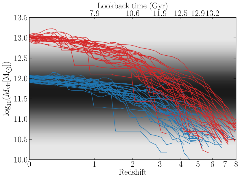
Figure 1: The large variation in the possible growth histories of haloes which all have approximately equal masses by redshift zero. The grey shaded region indicates the amplitude of the physics function in Eqn. 3. The blue and red lines represent 30 randomly selected growth histories for haloes with final $M_{\rm vir}$ values of approximately $10^{12}$ and $10^{13}\,M_{\sun}$, respectively. Variations of 3–4 Gyr in the time at which these haloes reach a given mass is common. Unlike statistical techniques for tying galaxy properties to their host haloes, our formation history model implicitly includes the full range of different halo growth histories and their effects on the predicted galaxy population.

In practice haloes of the same $z{=}0$ mass may show a diverse range of growth histories, all of which are captured by our model. In Fig. 1 we demonstrate this by showing the individual growth histories of a random sample of dark matter haloes selected from the Millennium Simulation in two narrow mass bins. From this figure we see that there can be significant variations in the time at which similar haloes at redshift zero reach a given mass. For example, in the upper halo mass sample, some haloes reach $10^{12}\,{\rm M_{\sun}}$ by $z{=}5$ whilst others do not reach this value until $z{=}2$. In addition, some haloes may have complex growth histories, achieving their maximum mass at $z{>}0$. This can potentially be caused by a number of processes such as stripping during dynamical encounters with other haloes. Since the baryonic growth function maps the formation history of each individual dark matter halo to the stellar mass growth of its galaxy, this diversity in growth histories is fully captured, propagating through to be reflected in the predicted galaxy populations at all redshifts. This is an important attribute of our model that sets it apart from other statistical-based methods which merely map the properties of galaxies to the instantaneous or mean properties of haloes, independently of their histories (e.g. HOD and SHAM models). These methods typically have to add artificial scatter to approximate the effects of variations in the halo histories, whereas this variation is a self-consistent input to our formation history model.

2.2.2 The physics function

The physics function describes the efficiency with which baryons are converted into stars in haloes of a given mass. The form of this function may be arbitrarily complex, however, the goal of this work is to find the simplest model which successfully ties the growth of galaxy stellar mass to the properties of the host dark matter haloes. The physics function is not meant to provide an accurate reproduction of the details of the full input physics, but rather their combined effects on the growth of stellar mass in the Universe. In this spirit, we begin by assuming that there is only one input variable: the instantaneous virial mass of the halo, $M_{\rm vir}$.

Although still not understood in detail, the observed relationship between dark matter halo mass and galaxy stellar mass is well documented (e.g. Zheng et al., 2007; Yang et al., 2012; Wang et al., 2013). Assuming the favoured $\Lambda{\rm CDM}$ cosmology, a comparison of the observationally determined galactic stellar mass function to the theoretically determined halo mass function indicates that the averaged efficiency of stellar mass growth varies strongly as a function of halo mass. In Fig. 2, we contrast a Schechter function fit of the observed redshift zero stellar mass function (solid blue line; Bell et al., 2003) against the dark matter halo mass function of the Millennium Simulation (red dashed line). The halo mass function has been multiplied by $f_{\rm b}$ in order to approximate the total amount of baryons available for star formation in a halo of any given mass.

The increased discrepancy between the stellar mass function and halo mass functions at both low and high masses indicates that the efficiency of star formation is reduced in these regimes. It is commonly held that at low masses the shallow gravitational potential provided by the dark matter haloes allows supernova feedback to efficiently eject gas and dust from the galaxy. This reduces the availability of this material to fuel further star formation episodes, hence temporarily stalling in situ stellar mass growth. Other processes such as the photoionization heating of the intergalactic medium may also play an important role in reducing the efficiency of star formation in this low-mass regime (Benson et al., 2002, and references therein). At high halo masses, it is thought that inefficient cooling coupled with strong central black hole feedback also leads to a quenching of star formation (e.g. Croton et al., 2006). Therefore, it is only between these two extremes, around the knee of the galactic stellar mass function, that stellar mass growth reaches its highest average efficiency.

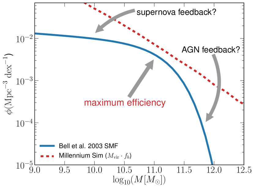
Figure 2: A comparison of the observed galactic stellar mass function (blue solid line) and the halo mass function of the Millennium Simulation (red dashed line). The halo mass function has been multiplied by the universal baryon fraction in order to demonstrate the maximum possible stellar mass content as a function of halo mass. The closer the stellar mass function is to this line, the more efficient star formation is in haloes of the corresponding mass. If galaxies were to form stars with a fixed efficiency at all halo masses then the slope of the stellar mass function would be identical to that of the halo mass function. The differing slopes at both high and low masses indicates that star formation (as a function of halo mass) is less efficient in these regimes. At low masses, this is commonly attributed to efficient gas ejection due to supernova feedback, whereas at high masses energy injection from central super-massive black holes is thought to be able to effectively reduce the efficiency of gas cooling. However, many other physical processes may also contribute in both regimes.

We begin by parametrizing the physics function as a simple log-normal distribution centred around a halo virial mass $M_{\rm peak}$, and with a standard deviation $\sigma_{M_{\rm vir}}$:

$$F_{\rm phys}(M_{\rm vir}/M_{\sun})=\mathcal{E}_{M_{\rm vir}}\exp\left(-\left(\frac{\Delta M_{\rm vir}}{\sigma_{M_{\rm vir}}}\right)^{2}\right),$$ (3)

where $\Delta M_{\rm vir}{=}\log_{10}(M_{\rm vir}/M_{\sun}){-}\log_{10}(M_{\rm peak}/M_{\sun})$ and the parameter $\mathcal{E}_{M_{\rm vir}}$ represents the maximum possible efficiency for converting in-falling baryonic material into stellar mass, achieved when $M_{\rm vir}{=}M_{\rm peak}$. Such a distribution has been found by SHAM studies to provide a good match to the derived star formation rates as a function of halo mass for $z{\la}2$ (Conroy & Wechsler, 2009; Béthermin et al., 2012).

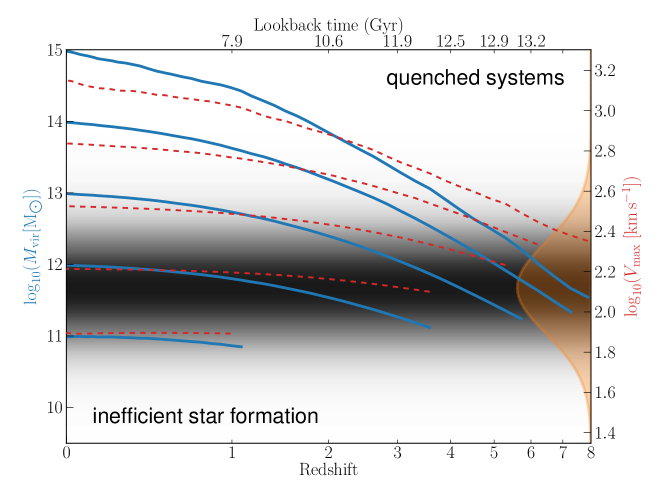
Figure 3: The mean virial mass ($M_{\rm vir}$) growth histories for five samples of dark matter haloes with varying final masses (blue solid lines). Each sample is only plotted out to a redshift limit determined by where 80% of the haloes contain more than 40 particles. The grey shaded region indicates the amplitude of the physics function in Eqn. 3. This is also illustrated by the log-normal curve on the right-hand side (orange shaded region). Galaxies with halo masses within the peaked region form stars efficiently; outside this mass range, the amount of star formation is negligible. All galaxies of sufficient mass at $z{=}0$ will cross the efficient star formation mass range at some point in their history, with this period typically coming earlier for more massive haloes. Also shown is the mean maximum circular velocity ($V_{\rm max}$) evolution for haloes of varying final velocity (red dashed lines). These samples have been chosen to have $z{=}0$ maximum circular velocity values similar to the mean values of the five mass-selected samples. There are clear differences in the evolution of $V_{\rm max}$ and $M_{\rm vir}$ which will in turn result in differences between the produced galaxy populations.

This simple form of the physics function provides a number of desirable properties. In Fig. 3, we present the average growth histories of five samples of dark matter haloes chosen from the Millennium Simulation merger trees by their final redshift zero masses (solid blue lines). For clarity, we only plot these histories out to redshifts where more than 80% of the haloes in each sample have masses which are twice the resolution limit of the input merger trees. The grey shaded region indicates the amplitude of the physics function defined by Eqn 3 when using our fiducial parameter values (see §3.1 for details). As the haloes grow, they pass through the region of efficient star formation at different times depending on their final masses. Galaxies hosted by the most massive $z{=}0$ haloes form the majority of their in situ stellar mass at earlier times whereas those in the lowest mass haloes are still to reach the peak of their growth. In addition, lower mass haloes tend to spend a longer time in the efficient star forming regime compared to their high-mass counterparts. These trends qualitatively agree with the observed phenomenon of galaxy downsizing (e.g. Cowie et al., 1996; Cattaneo et al., 2008).

Subhalo abundance matching studies have suggested that $V_{\rm max}$ may be more tightly coupled to the stellar mass growth of galaxies than $M_{\rm vir}$ (e.g. Reddick et al., 2013). This makes intuitive sense as $V_{\rm max}$ is directly related to the gravitational potential of the inner regions of the host halo, where galaxy formation occurs. Therefore, in addition to virial mass we also consider the case of a physics function where the dependent variable is the instantaneous maximum circular velocity of the host halo, $V_{\rm max}$:

$$F_{\rm phys}(V_{\rm max}/{\rm(km\,s^{-1})})=\mathcal{E}_{V_{\rm max}}\exp\left(-\left(\frac{\Delta V_{\rm max}}{\sigma_{V_{\rm max}}}\right)^{2}\right),$$ (4)

where $\Delta V_{\rm max}{=}\log_{10}(V_{\rm max}/{\rm(km\,s^{-1})}){-}\log_{10}(V_{\rm peak}/{\rm(km\,s^{-1})})$. To avoid confusion, from now on we will refer to the formation history model constructed using this physics function as the “static $V_{\rm max}$ model”. Similarly, we will refer to the case of $F_{\rm phys}(M_{\rm vir})$ as the “static $M_{\rm vir}$ model”.

In Fig. 3 we show the average $V_{\rm max}$ growth histories for a number of different $z{=}0$ selected samples. The $y$-axis has been scaled such that the grey band also correctly depicts the changing amplitude of the $V_{\rm max}$ physics function as well as its $M_{\rm vir}$ counterpart. Additionally, each of the $V_{\rm max}$ samples in Fig. 3 (red dashed lines) is chosen to have mean $z{=}0$ values close to that of the five $M_{\rm vir}$ samples (blue lines). However, there are clear differences between the growth histories of these two halo properties. In particular, the evolution of $V_{\rm max}$ is slightly flatter, resulting in haloes transitioning out of the efficient star forming region at an earlier time than the equivalent $M_{\rm vir}$ sample. Such differences will have important consequences for the time evolution of the galaxy populations generated by each of the two physics functions and we highlight some of these in §3.

By combining the baryonic growth function with a physics function of the forms presented here, our resulting model may be thought of as a simplified and extended version of that presented by Bouché et al. (2010). Unlike their model, the scaling of gas accretion efficiency with halo mass, and the dependence of star formation on previously accreted material, is implicitly contained within our physics function. Most importantly though, Bouché et al. (2010) use statistically generated halo growth histories instead of simulated merger trees. Hence their model contains no information about the scatter due to variations in halo formation histories. Furthermore, since their growth histories do not include satellites, there is no self-consistent stellar mass growth due to mergers.

The model of Cattaneo et al. (2011) also uses simulated merger trees as input and thus shares many of the same advantages as our formation history model. However, their model ties the properties of galaxies to the instantaneous properties of their host haloes alone. In contrast, we use the full information of the mass accretion history to describe the availability of baryonic material for star formation. Also, we make no attempt to motivate the precise form of our model in terms of combinations of particular physical processes and their scalings with halo properties, as Cattaneo et al. (2011) do. This allows our model to remain maximally general and flexible.

2.3 Generating the galaxy population

Armed with the forms of our baryonic growth function (Eqn. 2) and physics function (Eqn. 3), we now discuss the practical implementation of the formation history model to generate a galaxy population from the input dark matter merger trees.

For each halo in the tree, the change in dark matter halo mass, coupled with the time between each merger tree snapshot, provides us with the value of ${\rm d}M_{\rm vir}/{\rm d}t$. This change in mass naturally includes growth due to both smooth accretion and merger events. Combined with the instantaneous value of $M_{\rm vir}$ or $V_{\rm max}$ we can calculate a star formation rate for the occupying galaxy following Eqn. 1.

Some fraction of the mass formed by each new star formation episode will be contained within massive stars. The lives of these stars will be relatively short and therefore they will not contribute to the measured total stellar mass content of the galaxy. In order to model this effect we invoke the “instantaneous recycling” approximation (Cole et al., 2000), whereby some fraction of the mass of newly formed stars is assumed to be instantly returned to the galaxy interstellar medium (ISM). Based on a Salpeter (1955) IMF we take this fraction to be 30%, however, we note that changes to this value can be trivially taken into account by appropriately scaling the value of $\mathcal{E}$ in the physics function.

Although well motivated and conceptually simple, our use of ${\rm d}M_{\rm vir}/{\rm d}t$ in the baryonic growth function (Eqn. 2) does introduce some practical considerations. For example, the change in halo mass from snapshot-to-snapshot in the input dark matter merger trees can be stochastic in nature, especially for the case of low-mass or diffuse haloes identified in regions of high density. Also, when satellite galaxies fall into larger systems their haloes are tidally stripped, leading to a negative change in halo mass and thus a reduction in stellar mass according to Eqn. 1. In the real Universe, we expect that the galaxy is located deep within the potential well of its host halo and is therefore largely protected from the earliest stripping effects suffered by the dark matter (Peñarrubia et al., 2010). We must therefore decide when, if at all, to allow stellar mass loss when using this formalism. For simplicity, we address this by setting the star formation rate of satellite galaxies to be zero at all times; in other words fixing their stellar mass upon in fall. This is unlikely to be true in the real Universe across all mass and environment scales (Weinmann et al., 2006), however, the assumption of little or no star formation in satellite galaxies is a reasonable approximation and is relatively common in analytic galaxy formation models (e.g. Kauffmann et al., 1999; Cole et al., 2000; Bower et al., 2006; Croton et al., 2006). It is also in keeping with our goal of finding the simplest possible model.

The form of the baryonic growth function presented in Eqn. 2 above is only one of a number of possibilities. As an example, one could use the instantaneous halo mass divided by its dynamical time, $M_{\rm vir}/t_{\rm dyn}$. This quantity grows more smoothly over the lifetime of a halo and is never negative. Additionally, one may speculate that this is a better representation of the link between stellar and halo mass build up. However, for simplicity, we do not investigate alternative forms of the baryonic growth function, but leave this to future work.

Satellite galaxies are explicitly tracked in the input merger trees until their host subhaloes can no longer be identified or fall below the imposed resolution limit of 20 particles. At this point, their position is approximated by the location of the most bound particle at the last snapshot the halo was identified. We then follow Croton et al. (2006) in assuming that the associated satellite galaxy will merge with the central galaxy of the parent halo/subhalo after a time-scale motivated by dynamical friction arguments (Binney & Tremaine, 2008):

$$t_{\rm merge}=\frac{1.17}{G}\frac{V_{\rm vir}r^{2}_{\rm sat}}{m_{\rm sat}\ln(1+M_{\rm vir}/m_{\rm sat})}\ ,$$ (5)

where $V_{\rm vir}$ and $M_{\rm vir}$ are the virial velocity and mass of the parent dark matter halo in $\rm km\,s^{-1}$ and $\rm M_{\sun}$ respectively, $r_{\rm sat}$ is the current radius of the satellite halo in $\rm kpc$, and $m_{\rm sat}$ is the mass of the satellite in $\rm M_{\sun}$. In these units, the gravitational constant, $G$, is given by $\rm 4.40\times 10^{-9}\>kpc{{}^{2}}\,km\,s^{-1}\,M_{\sun}^{-1}\,Myr^{-1}$.

The final stellar mass of a merger remnant is given by the sum of the stellar masses of the two merging progenitor galaxies. This is a key feature of the model and allows the growth histories of the progenitors of each galaxy to affect the final stellar populations of their descendants. Our input dark matter merger trees are constructed such that the mass of central friends-of-friends haloes implicitly includes the mass of all of its associated subhaloes. Therefore, as an in-falling satellite halo crosses the virial radius of its parent, the satellite mass is instantaneously added to that that of the parent, thus contributing to its $dM_{\rm vir}/dt$ value and the amount of star formation in the central galaxy. In reality this burst of newly formed stars could be produced by a number of different mechanisms. These include star formation in the central galaxy fuelled by external smooth accretion or material stripped from the infalling satellite (e.g. hot halo gas), star formation in the satellite galaxy as it uses up its remaining cold gas reserves during infall and the merger-driven starburst which may occur when the central or satellite galaxies eventually do collide and merge. However, our simple model makes no assumptions about what contribution each of these mechanisms makes to the total amount of stars produced during a merger event.

Combined with our simple baryonic growth function that assumes all of the incoming baryonic material is available for star formation (irrespective of whether or not it is already locked up in stars), our model implicitly includes merger-driven starbursts with an increased efficiency. However, since we do not explicitly account for the amount of incoming baryons which are already locked up in stars when a satellite halo in-falls, there is the possibility that the resulting merger-driven star burst produces a system with a baryon fraction in excess of the universal value. For our best-fitting models below, we have found that this situation occurs in less than 0.25% of all friends-of-friends haloes at any single snapshot. The situation is most prevalent in haloes with $M_{\rm vir}{\approx}11.5\>M_{\sun}$, although even there, less than 1% have baryon fractions above the cosmic value.

Knowledge of the star formation rates of each galaxy and its progenitors at every time step in the simulation allows us to also calculate luminosities. For this purpose we use the simple stellar population models of Bruzual & Charlot (2003) and assume a Salpeter (1955) IMF. In the real Universe supernova ejecta enriches the intra galactic medium, altering the chemical composition of the next generation of stars and the spectrum of the light they emit. As we do not track the amount of gas or metals in our simple model, we assume all stars are of 1/3 solar metallicity. This is a common assumption when no metallicity information is available. Finally, a simple “plane-parallel slab” dust model (Kauffmann et al., 1999) is applied to the luminosity of each galaxy in order to provide approximate dust extincted magnitudes. These magnitudes are used below to augment our analysis by allowing us to calculate the $B{-}V$ colour for each galaxy at $z{=}0$. However, our main focus will remain on stellar masses as these are a direct model prediction.

3 Results

Having outlined the methodology and implementation of our simple formation history model, we now present some basic results which showcase its ability to recreate observed distributions of galaxy properties. We begin by considering redshift zero alone, before moving on to investigate the results at higher redshifts. Throughout, we contrast the variations between the predicted galaxy populations when using $M_{\rm vir}$ or $V_{\rm max}$ as the dependant variable of the physics function (Eqns. 3 & 4).

3.1 Redshift zero

Table 1: The fiducial parameter values of the physics function when using either $M_{\rm vir}$ or $V_{\rm max}$ as the dependant variable. Values are presented for both the non-evolving (see §3.1) and evolving (see §3.3) form. Also shown are the ranges for the flat priors used during the MCMC calibration. The parameters $\log_{10}(M_{\rm peak}/\rm{M_{\sun}})$ and $\log_{10}(V_{\rm peak}/({\rm km\,s^{-1})})$ indicate the haloes which possess the peak star formation efficiency (at $z{=}0$ in the evolving case). The $\sigma$ and $\mathcal{E}$ parameters represent the width and height of the Gaussian physics function, respectively. For the evolving models, $\alpha$, $\beta$ and $\gamma$ indicate the rate of power-law evolution of the peak location, width and height of the physics function, respectively. The non-evolving model parameters were chosen to provide the best reproduction of the observed $z{=}0$ colour-split stellar mass function of Bell et al. (2003). In the evolving case, the values were chosen to additionally reproduce the evolution of the peak stellar–halo mass relation of Moster et al. (2013).

$\mathbf{M_{\rm vir}}$ model	$\log_{10}(M_{\rm peak}/\rm{M_{\sun}})$	$\sigma_{M_{\rm vir}}$	$\mathcal{E}_{M_{\rm vir}}$	$\alpha_{M_{\rm vir}}$	$\beta_{M_{\rm vir}}$	$\gamma_{M_{\rm vir}}$
Prior ranges	[$11.15,12.65$]	[$0.2,1.5$]	[$0.1,1.5$]	[$-3.0,3.0$]	[$-3.0,3.0$]	[$-3.0,3.0$]
Static (§3.1.1)	$11.7$	$0.65$	$0.56$	–	–	–
Evolving (§3.3)	$11.6$	$0.56$	$0.90$	$0.03$	$0.25$	$-0.74$
$\mathbf{V_{\rm max}}$ model	$\log_{10}(V_{\rm peak}/({\rm km\,s^{-1})})$	$\sigma_{V_{\rm max}}$	$\mathcal{E}_{V_{\rm max}}$	$\alpha_{V_{\rm max}}$	$\beta_{V_{\rm max}}$	$\gamma_{V_{\rm max}}$
Prior ranges	[$1.5,3.5$]	[$0.1,1.5$]	[$0.1,1.5$]	[$-3.0,3.0$]	[$-3.0,3.0$]	[$-3.0,3.0$]
Static (§3.1.2)	$2.2$	$0.18$	$0.53$	–	–	–
Evolving (§3.3)	$2.1$	$0.17$	$1.12$	$0.10$	$0.33$	$-0.98$

In order to determine the “best” parameter values for the $M_{\rm vir}$ model, we calibrate them against Schechter function fits of the observed red and blue galaxy stellar mass functions of Bell et al. (2003). This calibration was done using Markov chain Monte Carlo (MCMC) parameter estimation techniques (for details of our implementation see Mutch et al., 2013). The observed mass functions are constructed from a $g$-band limited sample taken from a combination of Sloan Digital Sky Survey (SDSS) early release (Stoughton et al., 2002) and Two Micron All Sky Survey (2MASS; Jarrett et al., 2000) data, with a magnitude-dependent colour cut used to divide the red and blue galaxy populations. To similarly split the model galaxies into red and blue samples we employ a more basic mass/magnitude independent colour cut of $B{-}V=0.8$. This is equivalent to the colour division found by the 2dF Galaxy Redshift Survey (Cole et al., 2005).

For all of the results presented in this work we use a minimum of 130 000 model calls in the integration phase of our Monte Carlo chains, where the precise number used varies in proportion to the number of free model parameters. Due to computational limitations we are unable to utilize the full Millennium Simulation volume and instead restrict ourselves to a random sampling of 1/128 of the total simulation merger trees. This is equivalent to a comoving volume of approximately $9.8\times 10^{6}\mathrm{h}^{-3}\,\mathrm{Mpc^{3}}$ (i.e. a box with a side length of approximately $100\mathrm{h}^{-1}\,\mathrm{Mpc}$). We use the same random merger tree set throughout. Flat priors were used for each parameter with ranges as presented in Table 1. To ensure that all of our chains are fully converged we employ the Rubin–Gelman statistic (Gelman & Rubin, 1992) as well as visually inspect the chain traces.

It is important to note that, since our model relies on both the instantaneous host dark matter halo mass and its growth rate, the precise best-fitting parameter values may vary depending on the time-step spacing between the snapshots of the input simulation. For this reason one should be cautious not to over-interpret the exact parameter values of our simple model as they can be sensitive to the details of the implementation.

Using the posterior probability distributions of the MCMC fitting procedure allows us place 68 and 95% confidence limits on all of our model results, both constrained and predicted. In this work, confidence intervals are calculated from a large sample of model runs (60–200) that have parameter combinations randomly sampled from the relevant posterior distributions.

An important consideration when statistically calibrating any model against observational data is the use of realistic observational uncertainties (Mutch et al., 2013). As discussed by Bell et al. (2003), there is likely significant systematic uncertainties associated with their stellar mass function estimation which are not formally included in the relevant Schechter function parameter values. To overcome this we utilize the uncertainties of Baldry et al. (2008) which are calculated by comparing the global mass functions that result from five independent stellar mass determinations of a single galaxy sample. We then partition this global uncertainty between red and blue galaxies. This is done such that the fractional contribution to the uncertainty due to red (blue) galaxies is equal to the fraction of red (blue) galaxies in each stellar mass bin.

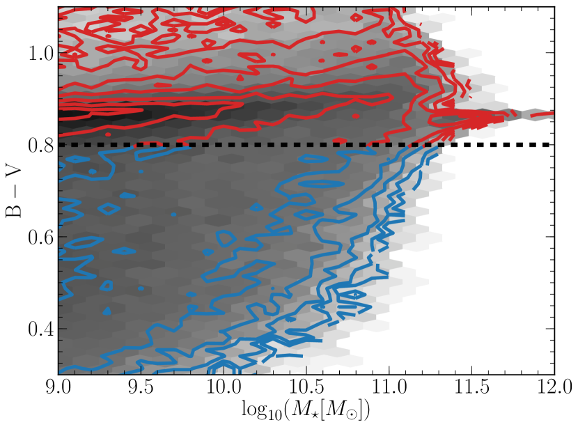
Figure 4: The colour–stellar mass diagram of the static $M_{\rm vir}$ model. The black dashed line at $B{-}V$=0.8 (Cole et al., 2005) indicates the value used to divide the model galaxies into red and blue samples. There is a clear ridge of over-density extending across all stellar masses at $B{-}V{\approx}0.87$ representing the red sequence.

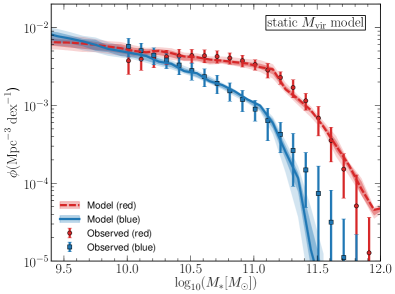
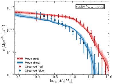
Figure 5: The red (dashed lines) and blue (solid lines) $z{=}0$ stellar mass functions produced by the static formation history model when using $M_{\rm vir}$ (left-hand panel) and $V_{\rm max}$ (right-hand panel) as the input variable to the physics function (Eqns. 3 & 4). Galaxy colour is classified using a mass-independent colour cut of $B{-}V{=}0.8$. The free model parameters have been calibrated to provide the best possible reproduction of the observed stellar mass function of Bell et al. (2003) (error bars) and are presented in Table 1. Shaded regions indicate the 68 (dark) and 95 (light) % confidence intervals of our MCMC fit. The fact that such an agreement can be achieved is an important success given the simplicity of the formation history model.

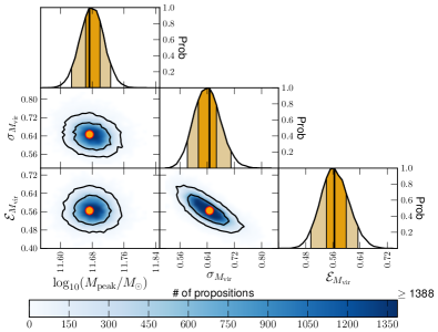
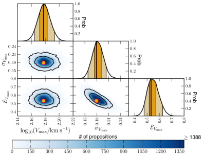
Figure 6: Marginalized posterior probability distributions for the $M_{\rm vir}$ (left) and $V_{\rm max}$ (right) static model parameters when calibrating against the red and blue stellar mass functions at $z{=}0$ (Fig. 5). All panels have been zoomed in to the high-probability regions. Contours on the 2D (blue) panels indicate the 68 and 95% confidence regions. Yellow dots mark the marginalized most probable parameter values. The diagonal panels show the marginalized 1D distributions with the 68 and 95% confidence intervals (dark and light shaded regions, respectively). The approximately Gaussian shape of these 1D distributions indicates the well behaved nature of the model. The only parameter degeneracies are between the normalization ($\mathcal{E}_{M_{\rm vir}}$/$\mathcal{E}_{V_{\rm max}}$) and width ($\sigma_{M_{\rm vir}}$/$\sigma_{V_{\rm max}}$) of the physics functions.

3.1.1 The $M_{\rm vir}$ model

The best-fitting parameters for the static $M_{\rm vir}$ model are presented in Table 1 (see §3.3 for the “evolving” model). The preferred $M_{\rm peak}$ value of $10^{11.7}\,\rm{M_{\sun}}$ implies that galaxies in haloes slightly less massive than that of the Milky Way ($M_{\rm vir}\approx 10^{12}\,\rm{M_{\sun}}$; Xue et al., 2008) are on average the most efficient star formers. In these haloes, 56% of all freshly accreted baryonic material is converted into stars, as indicated by the value of $\mathcal{E}_{M_{\rm vir}}$. We also note that both the position of the peak of the physics function and its width agree well with the star formation rate–halo mass relation obtained by the abundance matching study of Béthermin et al. (2012).

In Fig. 4 we show the colour–stellar mass diagram produced using the best parameters of our static $M_{\rm vir}$ model. The black dashed line indicates the colour split used to divide the galaxies into red and blue populations. Although there is a lack of a clear colour bi-modality as seen in observational data (e.g. Baldry et al., 2004), we still find a clear overabundance of galaxies with $B{-}V{\approx}0.87$ corresponding to the observed “red sequence”. The presence of this feature at approximately the correct position in colour space (Cole et al., 2005) is an interesting result for such a simple model.

In the left hand panel of Fig. 5 we show the red and blue model galaxy stellar mass functions (solid lines) against the corresponding constraining observations (error bars). Despite its simplicity, the chosen form of the physics function produces a good reproduction of the data. This is true across a wide range in stellar mass, indicating that the model is capable of successfully matching the integrated time evolution of stellar mass growth as a function of halo mass at $z{=}0$. Also, since blue galaxies preferentially trace those objects which have undergone significant recent star formation, the model’s reproduction of the observed blue mass function suggests that the rate of star formation as a function of stellar mass near $z{=}0$ is also in broad agreement with the observed Universe.

The fact that such an agreement is attainable with this simple model should be viewed as a key success of the methodology and a validation of the general form we have chosen for the physics function, $F_{\rm phys}(M_{\rm vir})$. Having said this, there are some differences in the left hand panel of Fig. 5 worth noting. In particular, there is an over-prediction in the number density of the most massive red galaxies and a corresponding under prediction of the most massive blue galaxies.

3.1.2 The $V_{\rm max}$ model

Having established that a physics function constructed using $M_{\rm vir}$ as the single input variable can successfully provide a good match to the observed $z{=}0$ red and blue stellar mass functions, we now turn our attention to the results of using $V_{\rm max}$ as the input property (Eqn. 4).

In the right hand panel of Fig. 5 we present the colour-split stellar mass functions for the static $V_{\rm max}$ model. Again, a fixed colour division of $B{-}V{=}0.8$ is used to define the two colour populations and we use MCMC tools to constrain the physics function parameter values to provide the best statistical reproduction of the Bell et al. (2003) data. The resulting parameter values are presented in Table 1. Unsurprisingly, a comparison with the equivalent values of the $M_{\rm vir}$ model indicates that the peak efficiency of converting fresh baryonic material into stars in a single time-step remains similar ($\mathcal{E}_{V_{\rm max}}{=}0.53;\,\mathcal{E}_{M_{\rm vir}}{=}0.56$). However, the average virial mass of haloes with $V_{\rm max}{\approx}(V_{\rm peak}{=}158\>\rm{km\,s^{-1}})$ is $10^{11.9}\,\rm{M_{\sun}}$, therefore this peak efficiency occurs in slightly more massive haloes than was the case for the $M_{\rm vir}$ model. This is a reflection of the different growth histories of these two halo properties.

As was the case for the $M_{\rm vir}$ model, an excellent reproduction of the observations is attainable when using $V_{\rm max}$ as the input parameter to the physics function. We find that the over prediction of high-mass red galaxies has been alleviated, although at the cost of now somewhat under predicting the number density of low-mass blue galaxies. Importantly though, given a suitable choice for values of the free parameters of the physics function, both the $M_{\rm vir}$ and $V_{\rm max}$ physics functions can produce a good match to the distribution and late time growth of stellar mass at $z{=}0$ despite the differences in their mean time evolution (cf. Fig. 3).

In Fig. 6 we present the marginalized posterior probability distributions for our MCMC calibration of both the $M_{\rm vir}$ (left-hand panel) and $V_{\rm max}$ (right-hand panel) models. For clarity we have zoomed in on the regions of high probability in all panels instead of showing the full ranges explored. The well behaved and understandable nature of the parameter distributions gives us further confidence in the validity of our model implementation. The approximately Gaussian shape of the 1D distributions (diagonal panels), coupled with their uni-modal nature, indicates that all of the parameters are well constrained. Furthermore, the 2D panels demonstrate that the only degeneracies in either model are between those parameters controlling the normalization ($\mathcal{E}_{M_{\rm vir}}$/$\mathcal{E}_{V_{\rm max}}$) and width ($\sigma_{M_{\rm vir}}$/$\sigma_{V_{\rm max}}$) of the log-normal physics function. This makes intuitive sense as these parameters jointly determine the integral of the star formation rate defined by Eqn. 1 and therefore the approximate total amount of stellar mass formed by each galaxy.

3.2 High redshift

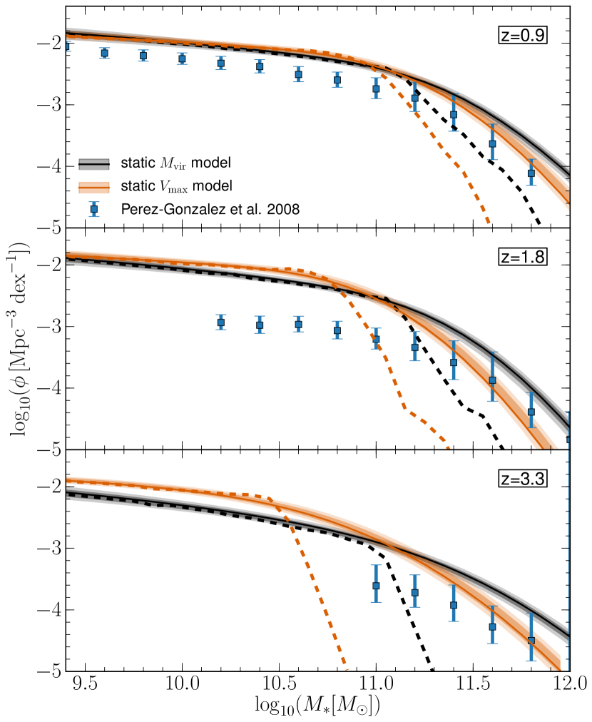
Figure 7: The $z{\approx}0.9$, 1.8, 3.3 stellar mass functions predicted by the static $M_{\rm vir}$ (dashed black line) and $V_{\rm max}$ (dashed orange line) models (Eqns. 3,4). Observational data from Pérez-González et al. (2008, PG08) and are shown for comparison. The solid lines indicate the results of convolving the model stellar masses with a normally distributed random uncertainty of 0.3 or 0.45 dex (for redshifts less than/greater than 3, respectively) in order to mimic the systematic uncertainties associated with the observed masses. The dark and light shaded regions show the 68 and 95% confidence intervals predicted using the marginalized parameter distributions obtained from our $z{=}0$ parameter calibration (Fig. 6). There are clear differences between the $M_{\rm vir}$ and $V_{\rm max}$ models at higher redshifts, despite their approximate agreement at $z{=}0$ (Fig. 5). This reflects the different time evolution of these two halo properties (see Fig. 3).

In the previous section we demonstrated that our simple formation history model is capable of reproducing the observed red and blue galaxy stellar mass functions of the local Universe. We also showed that this is true independent of whether we utilize the $M_{\rm vir}$ or $V_{\rm max}$ form of the physics function (Eqns. 3 & 4). However, as seen in Fig. 3, there are important differences in the time evolution of these halo properties. This suggests that we should see corresponding differences in the galaxy populations predicted at higher redshifts.

In Fig. 7 we present the stellar mass functions of both the $M_{\rm vir}$ and $V_{\rm max}$ models (dashed lines) against the observed $z{>}0$ mass functions of Pérez-González et al. (2008, points). The solid lines represent the formation history model results after a convolution with a normally distributed random error of dispersion 0.3 dex for $z{<}3$ and 0.45 dex for redshifts greater than this value (Moster et al., 2013). Such a convolution is common practice and approximates the missing uncertainties in the observational data due to systematics involved with producing stellar mass estimates from high-redshift galaxy observables (e.g. Fontanot et al., 2009; Guo et al., 2011; Santini et al., 2012).

There are clear quantitative differences between the stellar mass functions produced by the two models. These become more pronounced as we move to higher redshifts. At $z{\approx}3$ (bottom panel), the $V_{\rm max}$ model predicts a sharp fall off in the number density of galaxies with stellar masses greater than $10^{10.5}\,M_{\sun}$. When using $M_{\rm vir}$ to define the physics function, this drop off does not occur until $M_{\star}{\approx}10^{11}\,M_{\sun}$, resulting in a differing prediction in the number density of these galaxies by greater than two orders of magnitude at high masses. Despite this, both versions of the physics function predict $z{>}0$ stellar mass functions which are too steep at high masses, although the addition of the random uncertainties (solid lines) largely alleviates this problem. There are also notable differences at lower stellar masses, where both models over-predict the number of galaxies. The $V_{\rm max}$ model also predicts that a large fraction of galaxies with $M_{\rm vir}{<}10^{10.5}\,M_{\sun}$ are already in place by $z{=}3$, with a correspondingly slower evolution to $z{=}0$.

Many of these differing qualitative predictions can be understood by considering the differences in the time evolution of $M_{\rm vir}$ and $V_{\rm max}$ as shown in Fig. 3. For example, the deficit of high stellar mass galaxies in the $V_{\rm max}$ model at $z{\approx}3$ is due to their host haloes initially being identified with $V_{\rm max}$ values greater than $V_{\rm peak}$ (at least for the mass resolution of our simulation). These haloes therefore spend little time in the efficient star-forming band. The result is a reduced amount of in situ star formation at early times, with effects that carry all the way through to $z{=}0$ as these galaxies grow, predominantly through merging. We can similarly understand the cause of the larger predicted number density of high-redshift low-mass galaxies in the $V_{\rm max}$ model. In this case, the lowest mass haloes present at high redshifts have spent a longer time close to the peak of the efficient star-forming band. This results in these haloes already hosting significant amounts of stellar mass by $z{=}3$.

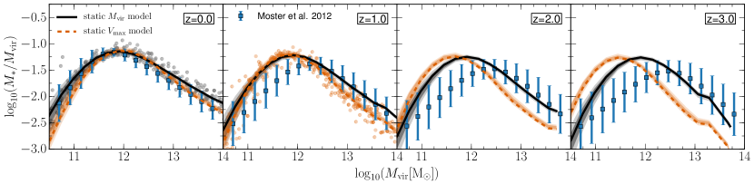
Figure 8: The evolution of the mean stellar–halo mass relation of central galaxies. The results of the static $M_{\rm vir}$ (Eqn. 3; black solid line) and $V_{\rm max}$ (Eqn. 4; orange dashed line) models are both shown. The dark and light shaded regions indicate the 68 and 95% confidence intervals predicted using the marginalized parameter distributions from our calibration at $z{=}0$ (see Fig. 6). A comparison with the subhalo abundance matching results of Moster et al. (2013) (blue error bars) indicates that both forms of the physics function fail to reproduce the evolution of the stellar mass growth efficiency required to reproduce the high-redshift stellar mass function (see Fig. 7). Coloured dots in the first and second panels show a random sampling of 20 galaxy–halo systems from each $x$-axis bin of the $M_{\rm vir}$ and $V_{\rm max}$ models, respectively.

To illustrate this further, in Fig. 8 we show the evolution of the mean stellar–halo mass relation for both models. The blue error bars represent the relations predicted by the subhalo abundance matching model of Moster et al. (2013). We have specifically chosen to compare our results against the work of Moster et al. (2013), as they take their halo masses from the same dark matter merger trees as used in this work (as well as the higher resolution Millennium-II Simulation; Boylan-Kolchin et al., 2009) and also construct their model to match the same high-redshift stellar mass functions of Pérez-González et al. (2008). Hence, the blue error bars of Fig. 8 represent the evolution in the integrated stellar mass growth efficiency which our model must achieve in order to successfully replicate the observed stellar mass functions of Fig. 7.

By construction, both the $M_{\rm vir}$ and $V_{\rm max}$ models produce extremely similar relations at $z{=}0$ but with clear differences at higher redshifts. It is these variations in the typical amount of stars formed within haloes of a given mass that drives the different predictions for the evolution of the stellar mass function. For example, the much higher average stellar mass content of low-mass haloes at $z{=}3$ when using the $V_{\rm max}$ model (Fig. 8) is the cause of the increased normalization of the low-mass end of the relevant stellar mass function in Fig. 7.

Importantly, it can be seen from Fig. 8 that neither the $M_{\rm vir}$ nor the $V_{\rm max}$ model reproduces the evolution of the stellar–halo mass relation found by Moster et al. (2013); in particular the position and normalization of the peak value. The use of a redshift-independent halo mass to define the peak in situ star formation efficiency of the $M_{\rm vir}$ model results in no change to the position of the peak of the stellar–halo mass relation with redshift. Although not immediately obvious why this should be so, it can be understood by considering the typical evolution of a halo across the relation.

At early times, haloes grow in mass rapidly, however, they typically still sit below the efficient star formation mass regime defined by the physics function (see Fig. 3). In Fig. 8, these haloes will therefore travel almost horizontally from left to right with a low stellar–halo mass fraction. Eventually haloes will enter the mass regime of efficient star formation, causing them to rapidly increase their stellar–halo mass fractions with only a relatively modest growth in halo mass. This phase of rapid stellar mass growth causes a ”pile-up” of galaxies in the stellar–halo mass relation that peaks around the virial mass at which haloes again transition out of the efficient star forming regime. Since the mass at which this occurs is fixed in our simple static model, the position of the stellar–halo mass relation peak is therefore also fixed in the $M_{\rm vir}$ model. Due to the evolving $M_{\rm vir}$–$V_{\rm max}$ relationship, the position of the peak efficiency for the $V_{\rm max}$ model does evolve, but unfortunately in the direction opposite to that required. The shallower tail of the relation towards higher halo masses is caused by the subsequent growth of galaxies due to mergers.

As well as the precise shape and normalization of the mean stellar–halo mass relation, it is also important to consider the scatter of the distribution about this mean. For example, at high halo masses it is possible to increase the scatter of stellar–halo mass ratios to produce an increased normalization of the high-mass end of the stellar mass function whilst leaving the mean stellar–halo mass relation unchanged. In the first two panels of Fig. 8 we have plotted the stellar–halo mass ratios of 20 randomly selected haloes from each of the 15 mass bins used to construct the mean relations. At halo masses above the peak value we find an approximately constant value for the scatter as a function $M_{\rm vir}$ in both models. Below the peak halo mass, the scatter rapidly increases with decreasing $M_{\rm vir}$. This reflects the stochastic nature of star formation for lower mass haloes whose mass evolution may not be well resolved at all times in our model. However, at $z{=}0$ we find an average 1$\sigma$ scatter of 0.15 for the $M_{\rm vir}$ model and 0.23 for the $V_{\rm max}$ model over the range of halo masses plotted. This agrees well with previous studies (e.g. More et al., 2009; Yang et al., 2009; Behroozi et al., 2013b).

Based purely on the inability to reproduce the required evolution in the stellar–halo mass relation, it is unlikely that the non-evolving physics function will be able to match the observed distribution of stellar masses in both the low- and high-redshift Universe simultaneously. This is true irrespective of the values of the available parameters or whether $M_{\rm vir}$ or $V_{\rm max}$ is used as the dependant variable.

3.3 Incorporating a redshift evolution

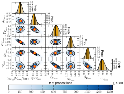
Figure 9: Marginalized posterior probability distributions for the $M_{\rm vir}$ (left) and $V_{\rm max}$ (right) parameters of the redshift dependent physics function. In both panels, the models were constrained to simultaneously reproduce the observed $z{=}0$ red and blue stellar mass functions (Fig. 12) as well as the time evolution of the stellar–halo mass relation (Fig. 9). All panels have been zoomed in to the high-probability regions. Con tours on the 2D (blue) panels indicate the 68 and 95% confidence regions. Yellow dots mark the marginalized most probable parameter values. The diagonal panels show the marginalized 1D distributions with the 1$\sigma$ and 2$\sigma$ confidence intervals shown by light and dark shaded regions, respectively. The approximately Gaussian shape of these 1D distributions indicates the well behaved nature of the model.

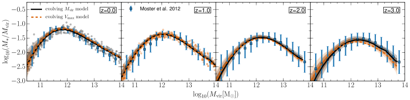
Figure 10: The evolution of the mean stellar–halo mass relation of central galaxies for the evolving $M_{\rm vir}$ (Eqn. 3; black solid line) and $V_{\rm max}$ (Eqn. 4; grey dashed line) models. Orange shaded regions indicated the subhalo abundance matching results of Moster et al. (2013). A comparison with Fig. 8 indicates that by shifting both the normalization ($\mathcal{E}_{M_{\rm vir}}$, $\mathcal{E}_{V_{\rm max}}$) and position ($M_{\rm peak}$, $V_{\rm peak}$) of the physics functions, we are able to reproduce the correct evolution of the stellar–halo mass relation at high-redshifts in terms of both shape and amplitude. This leads to a much better agreement between the observed and predicted stellar mass functions at $z{>}0$. (see Fig. 11). Coloured dots in the first and second panels show a random sampling of 20 galaxy/halo systems from each x-axis bin of the $M_{\rm vir}$ and $V_{\rm max}$ models respectively.

Although capable of reproducing the observed red and blue stellar mass functions at $z{=}0$, we showed in §3.2 that our simple formation history model struggles to reproduce the high-redshift distribution of stellar masses. Importantly, we also concluded that there is unlikely to be any combination of physics function parameter values (see Eqns. 3 & 4) which could alleviate this discrepancy. In this section we therefore look to extend our simple model by introducing a redshift dependence to the physics function. This is equivalent to the introduction of an evolution of the star formation efficiency with time for a fixed halo mass/maximum circular velocity. Such an evolution is well motivated both theoretically and observationally, suggesting the presence of alternative/additional star formation mechanisms at high-redshift when compared to those of the local Universe. For example, so-called “cold-mode” accretion (Birnboim & Dekel, 2003; Kereš et al., 2005; Brooks et al., 2009) is thought to be able to effectively fuel galaxies of massive haloes at high-redshift, allowing for increased star formation. In addition, the early Universe was a more dynamic place with an enhanced prevalence of gas-rich galaxy mergers and turbulence-driven star formation (e.g. Dekel et al., 2009; Wisnioski et al., 2011).

To reproduce the evolving position and normalization of the stellar–halo mass relation as found by Moster et al. (2013), we modify the physics function of Eqn. 3 by introducing a simple power law dependence on redshift to each of the free parameters:

$$\log_{10}(M_{\rm peak}(z)) = \log_{10}(M_{\rm peak})(1+z)^{\alpha_{M_{\rm vir}}}\ ,$$ (6)

$$\sigma_{M_{\rm vir}}(z) = \sigma_{M_{\rm vir}}(1+z)^{\beta_{M_{\rm vir}}}\ ,$$ (7)

$$\mathcal{E}_{M_{\rm vir}}(z) = \mathcal{E}_{M_{\rm vir}}(1+z)^{\gamma_{M_{\rm vir}}}\ ,$$ (8)

where at $z{=}0$: $M_{\rm peak}$$(z){=}$$M_{\rm peak}$, $\sigma_{M_{\rm vir}}$$(z){=}$$\sigma_{M_{\rm vir}}$ and $\mathcal{E}_{M_{\rm vir}}$$(z){=}$$\mathcal{E}_{M_{\rm vir}}$. The exact values of the redshift scalings are calibrated using MCMC to provide the best simultaneous reproduction of the Moster et al. (2013) stellar–halo mass relation at $z{=}0$, 1, 2 and 3, as well as the $z{=}0$ red and blue stellar mass functions, and are presented in Table 1.

In the left hand panel of Fig. 9 we present the relevant marginalized posterior probability distributions of the six free model parameters. Similarly to the redshift-independent case (cf. §3.1), the approximately Gaussian shape of the 1D probability distributions indicates that the parameters are generally well constrained. However, in addition to the degeneracy between the physics function normalization ($\mathcal{E}_{M_{\rm vir}}$) and width ($\sigma_{M_{\rm vir}}$) noted in §3.1, there are also clear and understandable degeneracies between the redshift evolution and $z{=}0$ value of each parameter (e.g. $M_{\rm peak}$ and $\alpha_{M_{\rm vir}}$).

We note that there are minor differences between the $z{=}0$ stellar mass function utilized by Moster et al. (2013) to constrain their stellar–halo mass relation (Li & White, 2009), and the $z{=}0$ mass function which we employ in this work (Bell et al., 2003). However, we calibrate our model against both the stellar–halo mass relation and colour-split stellar mass functions at $z{=}0$ with equal weights. The MCMC fitting procedure then attempts to find the best compromise between these two (as well as all other) constraints. Since we find that there are no multimodal features in the marginalized posterior probability distributions (see Fig. 9), the parameter sets required to fit each constraint individually must be statistically compatible with each other. We therefore conclude that this slight inconsistency in our fitting procedure has minimal effect on our ability to demonstrate the success and utility of the model and on our results.

The preferred values of $\alpha_{M_{\rm vir}}$ and $\beta_{M_{\rm vir}}$ are relatively small, indicating little need for evolution in both the peak position, $M_{\rm peak}$$(z)$, and width, $\sigma_{M_{\rm vir}}$$(z)$, of the physics function. As a consequence, the values of both $M_{\rm peak}$ and $\sigma_{M_{\rm vir}}$ are similar to the non-evolving case (cf. Table 1). However, there is a strong evolution preferred for the normalization of the physics function, $\gamma_{M_{\rm vir}}$, such that it decreases rapidly with increasing redshift. In order to maintain the total $z{=}0$ stellar mass density, the value of $M_{\rm peak}$=0.9 is therefore considerably higher than was the case in the non-evolving form of the physics function. This implies that 90% of all freshly accreted baryonic material in haloes with $\log_{10}(M_{\rm peak}/M_{\sun}){=}11.6$ is converted into stars at $z{=}0$. However, at $z{=}1$,2 and 3 the peak conversion efficiencies are considerably lower: 54, 40 and 32%, respectively.

We also similarly modify the $V_{\rm max}$ physics function, $F_{\rm phys}(V_{\rm max})$:

$$\log_{10}(V_{\rm peak}(z)) = \log_{10}(V_{\rm peak})(1+z)^{\alpha_{V_{\rm max}}}\ ,$$ (9)

$$\sigma_{V_{\rm max}}(z) = \sigma_{V_{\rm max}}(1+z)^{\beta_{V_{\rm max}}}\ ,$$ (10)

$$\mathcal{E}_{V_{\rm max}}(z) = \mathcal{E}_{V_{\rm max}}(1+z)^{\gamma_{V_{\rm max}}}\ ,$$ (11)

with the redshift scalings being calibrated to reproduce the same observations as the $M_{\rm vir}$ case above. The marginalized posterior probability distributions are presented in the right-hand panel of Fig. 9, with the preferred parameter values again presented in Table 1.

As was found for the redshift-dependent $M_{\rm vir}$ model, the marginalized posterior distributions indicate that the free model parameters are well constrained and that there are no unexpected degeneracies between them (Fig. 9). If we consider the preferred values of the parameters themselves, we again find that the normalization of the physics function, $\mathcal{E}_{V_{\rm max}}$$(z)$, shows the most pronounced evolution. A value of $\gamma_{V_{\rm max}}{=}-0.98$ indicates that the maximum star formation efficiency declines almost linearly as a function of $(1{+}z)$. This strong evolution requires a value of $\mathcal{E}_{V_{\rm max}}$ at $z{=}0$ that is actually greater than 1, and hence more than the total freshly accreted baryonic material must be converted into stars in haloes with $\log_{10}(V_{\rm peak}/{\rm(km\,s^{-1})}){=}2.1$ at this redshift. This suggests that we may need to vary the universal baryon fraction as a function of halo mass (or maximum circular velocity), perhaps to mimic the effects of processes such as the recycling of ejected baryons during star formation (e.g. Papastergis et al., 2012).

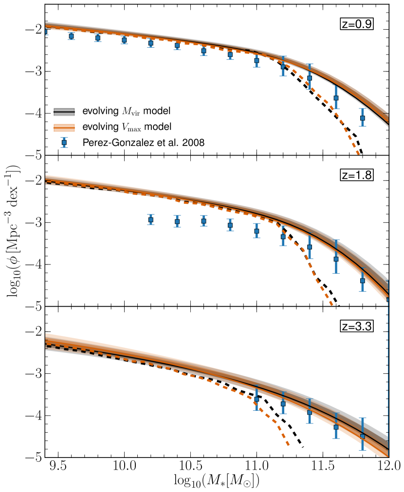
Figure 11: The $z{\approx}0.9$, 1.8, and 3.3 stellar mass functions predicted by the evolving $M_{\rm vir}$ (dashed black line) and $V_{\rm max}$ (dashed orange line) models. Observational data from Pérez-González et al. (2008) are shown for comparison. The solid lines give the results of convolving the model stellar masses with a normally distributed random uncertainty of 0.3 or 0.45 dex (for redshifts less than/greater than 0.3, respectively) in order to mimic the systematic uncertainties associated with the observed masses. By using an appropriate redshift evolution of the physics function parameters, the model’s ability to successfully recover the observed high-redshift stellar mass functions is improved.

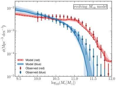
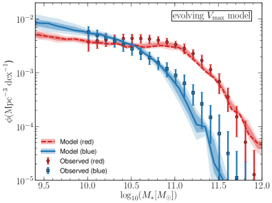
Figure 12: The red (dashed lines) and blue (solid lines) galaxy stellar mass functions produced by the evolving $M_{\rm vir}$ (left) and $V_{\rm max}$ (right) formation history models. Error bars indicate the observations of Bell et al. (2003). The free model parameters have been constrained to simultaneously reproduce these mass functions as well as the evolution of the stellar–halo mass relation (Fig. 10). The dark and light shaded regions show the associated 68 and 95% confidence regions obtained from this calibration.

In Fig. 10, we present the stellar–halo mass relations of the new, redshift-dependant, $M_{\rm vir}$ (black) and $V_{\rm max}$ (orange) models. The blue error bars again indicate the results of Moster et al. (2013). By incorporating the redshift dependence we are now able to successfully reproduce the evolution of both the normalization and peak position of the stellar–halo mass relation required at $z{\geq}0$. The effects of this on the predicted high-redshift stellar mass functions of both the $M_{\rm vir}$ and $V_{\rm max}$ models can be seen in Fig. 11. As expected, we now find an improved agreement with the observations when compared to the original, non-evolving physics function results (cf. Fig. 7). The typical 1$\sigma$ scatter in the evolving $M_{\rm vir}$ stellar–halo mass relation remains unchanged from the static case at approximately 0.15 dex at $z{=}0$. However, the scatter in the evolving $V_{\rm max}$ model is reduced to approximately 0.19 dex (from 0.23 dex in the static case). In both models the scatter decreases as a function of redshift such that at $z{=}1$ and $2$ it is approximately 0.13 and 0.01 dex, respectively.

For completeness we also present the $z{=}0$ colour-split stellar mass functions for both models in Fig. 12. A reasonable agreement with the constraining observational data is still achieved. However, we now find that an underprediction in the number density of massive blue galaxies is present in both models, suggesting that our implemented evolutionary model may not provide enough late time star formation in the most massive haloes.

4 Discussion

In §3.1, we demonstrated that our most basic, non-evolving form of the physics function is able to successfully reproduce the observed red and blue stellar mass functions of the local Universe (Fig. 5). This key result highlights the utility and validity of our basic methodology and model implementation. In addition, it reinforces the commonly held belief that the growth of galaxies is intrinsically linked to the growth of their host dark matter haloes (White & Rees, 1978).

Although the level of agreement achieved with the observed $z{=}0$ colour-split stellar mass functions is generally very good, there are some discrepancies. For example, there is an underprediction in the number density of the most massive blue galaxies in the $M_{\rm vir}$ model (left-hand panel of Fig. 5), with a corresponding overprediction in the number of massive red galaxies. Our $z{>}0$ analysis suggests that this is at least partially due to an incorrect evolution of the stellar–halo mass relation with time (see Fig. 8). However, we also note that an excess of massive red galaxies is a common feature of traditional semi-analytic galaxy formation models which similarly tie the evolution of galaxies to the masses of their host dark matter haloes. In such models, efficient feedback from AGN is typically responsible for truncating star formation in the most massive galaxies and hence causes the average stellar populations of these objects to become older and redder (Bower et al., 2006; Croton et al., 2006; Mutch et al., 2011). This is already mimicked within the framework of our formation history model through the turnover at the high $M_{\rm vir}$ (or $V_{\rm max}$) end of the physics function. However, a more gradual cut-off may be required in the $M_{\rm vir}$ model case, in order to allow star formation to proceed for longer in the galaxies populating the most massive haloes.

In this paper we have deliberately restricted ourselves to considering only a very simple form of the physics function. This has allowed us to take advantage of the resulting transparency when interpreting our findings. However, we stress that the model can easily be extended to include arbitrary levels of complexity. For example, we have chosen to use a log-normal distribution to define the form of the physics function. Although being conceptually simple, the symmetric nature of this formalism implicitly assumes that the physical mechanisms responsible for quenching star formation in both low- and high-mass haloes scale identically with halo mass (Fig. 3). This assumption has little physical justification and in order to provide the best results, it may be necessary to independently adjust the slope of the function at both low and high masses, and perhaps even as a function of redshift. In future work, we will address this issue by carrying out a full statistical analysis aimed at testing a number of different functional forms for both the physics and baryonic growth functions.

Even within the reduced scope of this current work, we have learned a great deal from simply examining the high-redshift stellar mass function predictions of the formation history model. In particular, we have highlighted the need for the physics function to produce an evolution in the stellar–halo mass relation as a function of redshift in order to match the observed space density of massive galaxies at early times. Using $V_{\rm max}$ as the input property to the function introduces such an evolution, but in the wrong direction. Future improvements to the model could focus on finding a halo property that does evolve correctly with time and would thus be a more natural anchor of the physics function. This would avoid the need to artificially introduce an evolution to match the observations, as we have done here.

Although the need for an evolving stellar–halo mass relation has been discussed in the literature, the precise form with which this evolution manifests itself is less clear. The results of subhalo abundance matching studies, such as that of Moster et al. (2013) (which we compare to in this work), are quite sensitive to the choice of input data sets and the technical aspects of the methodology. For example, Moster et al. (2013) find that the peak stellar–halo mass ratio increases from just 0.15% at ${z=}4$ to 4% at $z{=}0$, with a corresponding shift in position from a halo mass of $10^{12.5}\,{\rm M_{\sun}}$ to $10^{11.8}\,{\rm M_{\sun}}$. In contrast, an alternative study carried out by Behroozi et al. (2013b) finds very little change in either the normalization or peak location over a broad range in redshift. However, they do note a marked drop in the relation for the most massive haloes at $z{\la}2.5$. This results in a qualitatively different prediction for the evolution of these massive haloes, such that their efficiency of converting baryons in to stars is higher as a function of look-back time (the opposite trend to that found by Moster et al., 2013).

A potentially valuable use for the formation history model is to provide a general consistency check of subhalo abundance matching studies. The physics function could be adapted to exactly replicate the shape and evolution of the star formation efficiencies they predict (Behroozi et al., 2013a), allowing their validity to be assessed when self-consistently applied to individual dark matter merger trees. The additional galaxy properties provided by the formation history model, such as star formation histories and colours, could be used to further compare and contrast the success of different abundance matching methodologies. For example, it has been suggested that galaxy mergers may result in a significant fraction of the in-falling satellite stellar mass being added to a diffuse ICL component instead of to the newly formed galaxy (Monaco et al., 2006; Conroy et al., 2007). The strength of this effect is expected to increase significantly with increasing halo mass and is included in the subhalo abundance matching study of Behroozi et al. (2013b) but not Moster et al. (2013). By simply adding a mass-dependent amount of stellar material to an ICL component during merger events, our simple formation history model could be easily adapted to explore such a scenario.

We also note that the simplicity of our formation history model results in it being extremely fast and computationally inexpensive when compared to traditional semi-analytic models. This has allowed us to straightforwardly calibrate it against a number of observed relations using MCMC techniques. This procedure can also be trivially extended to provide statistically accurate (against select observations) mock catalogues for use with large surveys. Further to what can be achieved using current HOD or subhalo abundance matching methods, catalogues produced using our model include both full growth histories and star formation rate information for each individual galaxy, with no need to add any artificial scatter to approximate variations in formation histories. In addition, the direct and clear dependence of the model on the halo properties of the input dark matter merger trees makes it an ideal tool for investigating a number of additional topics. Examples include comparing the effects of variations between different $N$-body simulations and halo finders on the physics of galaxy formation and evolution, investigating the predictions of simple monolithic collapse scenarios, contrasting various mass-dependent merger starburst models and exploring the ramifications of $N$-body simulations run with alternative theories of gravity.

Finally, we note that a common criticism of semi-analytic models is the presence complex degeneracies between large numbers of free parameters. The MCMC calibration procedure we employ highlights the complete absence of such degeneracies in our formation history model, further demonstrating its well behaved and understandable nature.

4.1 Potential model extensions

One area of the model presented in this work which may benefit from being extended is the treatment of mergers (cf. §2.3). In the current model, merger-driven starbursts occur immediately when an infalling satellite halo crosses the virial radius of its parent. All of the newly formed stars are then added to the central galaxy of the parent halo. However, it is likely that there will be a significant time delay between the satellite crossing the virial radius of the parent and the actual merger between the satellite and central galaxy. In practice, due to the relatively large temporal spacing of our input dark matter merger trees (${\approx}200{-}350\,{\rm Myr}$), we expect this slight inconsistency to have little effect on our results. However, if running the formation history model on merger trees with a higher temporal resolution, this issue may become important. A future investigation of the clustering predictions of the formation history model, especially when split by galaxy colour, will allow us to fully assess the validity of these simplifications.

Also, as discussed in §2.3, we assume that all freshly accreted baryonic material is available for star formation, regardless as to whether or not it is already locked up in stars in the form of an infalling satellite galaxy. In practice this simply leads to an increased star formation efficiency for merger events. Testing of an alternative model in which the d$M_{\rm vir}$ term of the baryonic growth function includes only smooth accretion (i.e. does not include mass increases due to the accretion of satellite haloes) and star formation is allowed to proceed in satellite galaxies, indicates that merger-driven starbursts are an important feature of our model. Without this efficient star formation mechanism there is no combination of the available free parameters that allows the static model to reproduce the local colour-split stellar mass function.

Another potential extension of the current model would be to track the cold gas content of each galaxy. This would allow star formation to be limited to using only that gas which is currently available and not already locked up in stars, thus providing more realistic instantaneous star formation rates for individual galaxies. Merger-driven starbursts could additionally be implemented as consuming some fraction of any available cold gas in the two progenitor galaxies. More advanced versions of this class of model have already been shown to be successful in reproducing the results of full hydrodynamic simulations (Neistein et al., 2012), and have been explored in other works using statistically generated mass accretion histories (e.g. Bouché et al., 2010). However, it is important to recognize that our aim with the formation history model is to provide a simple, physically motivated, “toy” model. By adding the ability to track various reservoirs of material, or other similar complexities, we would arrive at what is essentially a simplified semi-analytic galaxy formation model, which is not the goal of this work.

5 Conclusions

In this work we introduce a simple model for self-consistently connecting the growth of galaxies to the formation history of their host dark matter haloes. This is achieved by directly tying the time averaged change in mass of a halo to the star formation rate of its galaxy via two simple functions: the “baryonic growth function” and the “physics function” (Eqns. 2,3). We utilize $N$-body dark matter merger trees to provide self-consistent growth histories of individual haloes that naturally includes scatter due to varying formation histories. This allows us to produce full star formation histories for individual objects, and thus provide predictions for secondary properties such as galaxy colour.

While closely related to other models in terms of its basic methodology (Bouché et al., 2010; Cattaneo et al., 2011), our model has a number of important generalizations which enhance its utility. In particular, we implement a single, unified physics function which encapsulates the effects of all of the intertwined baryonic processes associated with galactic star formation and condenses them down into a simple mapping between star formation efficiency and dark matter halo properties. The qualitative form of this function is motivated by our general knowledge of galaxy evolution, however, in this work we make no attempt to directly tie it to individual physical processes or their particular scalings with halo properties.

As well as introducing this new model, we demonstrate its ability to replicate important observed relations such as the galactic stellar mass function, and also illustrate some examples of its potential for investigating different theories of galaxy formation and evolution. Our main results can be summarized as follows.

1. Motivated by the observed suppression of star formation efficiency in both the most massive and least massive dark matter haloes we begin by parametrizing the physics function as a simple, non-evolving, log-normal distribution with a single independent variable of either halo virial mass, $M_{\rm vir}$, or maximum circular velocity, $V_{\rm max}$ (Fig. 3).

2. With just three free parameters controlling the position, normalization and dispersion of the peak star formation efficiency, we show that the formation history model can successfully reproduce the observed red and blue stellar mass functions at redshift zero. Assuming a suitable choice of the parameters, this result is independent of the use of $M_{\rm vir}$ or $V_{\rm max}$ as the dependant variable of the physics function (Fig. 5).

3. For the purposes of replicating the stellar mass functions across a wide range of redshifts, we find our static model to be inadequate. This is due to its inability to produce the correct evolution of the stellar–halo mass relation with time (Figs 7 and 8).

4. We therefore investigate the use of redshift as a second dependant variable to the physics function in order to control the position and normalization of the peak star formation efficiency with time. Using this simple adaptation alone, the formation history model is able to better reproduce the observed high-redshift stellar mass functions out to $z{=}3.5$ (Figs 10 and 11) whilst still maintaining a good reproduction of the $z{=}0$ colour-split stellar mass function.

5. By statistically calibrating the free model parameters using MCMC techniques throughout this work, we are able to use the marginalized posterior likelihood distributions to demonstrate the well behaved and transparent nature of our simple model (Fig. 6).

In order to demonstrate its construction and utility we have presented one of the simplest forms of the formation history model. However, a fundamental strength of its construction is that it can be easily extended to arbitrary levels of complexity in order to investigate a whole host of physical processes associated with galaxy formation and evolution, some general examples of which we have outlined in §4. In future work we will investigate the predictions made when using alternative forms of the baryonic growth and physics functions. We will also extend the model to investigate the birth of super-massive black holes and the evolution of the quasar luminosity function.

References

- Baldry et al. (2004) Baldry I. K., Glazebrook K., Brinkmann J., Ivezić Ž., Lupton R. H., Nichol R. C., Szalay A. S., 2004, ApJ, 600, 681
- Baldry et al. (2008) Baldry I. K., Glazebrook K., Driver S. P., 2008, MNRAS, 388, 945
- Behroozi et al. (2013a) Behroozi P. S., Wechsler R. H., Conroy C., 2013a, ApJ, 762, L31
- Behroozi et al. (2013b) Behroozi P. S., Wechsler R. H., Conroy C., 2013b, ApJ, 770, 57
- Bell et al. (2003) Bell E. F., McIntosh D. H., Katz N., Weinberg M. D., 2003, ApJS, 149, 289
- Benson et al. (2002) Benson A. J., Lacey C. G., Baugh C. M., Cole S., Frenk C. S., 2002, MNRAS, 333, 156
- Béthermin et al. (2012) Béthermin M., Doré O., Lagache G., 2012, A&A, 537, L5
- Binney & Tremaine (2008) Binney J., Tremaine S., 2008, Galactic Dynamics: Second Edition. Princeton University Press
- Birnboim & Dekel (2003) Birnboim Y., Dekel A., 2003, MNRAS, 345, 349
- Bouché et al. (2010) Bouché N. et al., 2010, ApJ, 718, 1001
- Bower et al. (2006) Bower R. G., Benson A. J., Malbon R., Helly J. C., Frenk C. S., Baugh C. M., Cole S., Lacey C. G., 2006, MNRAS, 370, 645
- Boylan-Kolchin et al. (2009) Boylan-Kolchin M., Springel V., White S. D. M., Jenkins A., Lemson G., 2009, MNRAS, 398, 1150
- Brooks et al. (2009) Brooks A. M., Governato F., Quinn T., Brook C. B., Wadsley J., 2009, ApJ, 694, 396
- Bruzual & Charlot (2003) Bruzual G., Charlot S., 2003, MNRAS, 344, 1000
- Cattaneo et al. (2008) Cattaneo A., Dekel A., Faber S. M., Guiderdoni B., 2008, MNRAS, 389, 567
- Cattaneo et al. (2011) Cattaneo A., Mamon G. A., Warnick K., Knebe A., 2011, A&A, 533, A5
- Cole et al. (2000) Cole S., Lacey C. G., Baugh C. M., Frenk C. S., 2000, MNRAS, 319, 168
- Cole et al. (2005) Cole S. et al., 2005, MNRAS, 362, 505
- Conroy & Wechsler (2009) Conroy C., Wechsler R. H., 2009, ApJ, 696, 620
- Conroy et al. (2006) Conroy C., Wechsler R. H., Kravtsov A. V., 2006, ApJ, 647, 201
- Conroy et al. (2007) Conroy C., Wechsler R. H., Kravtsov A. V., 2007, ApJ, 668, 826
- Cowie et al. (1996) Cowie L. L., Songaila A., Hu E. M., Cohen J. G., 1996, AJ, 112, 839
- Croton et al. (2006) Croton D. J. et al., 2006, MNRAS, 365, 11
- Dekel et al. (2009) Dekel A. et al., 2009, Nature, 457, 451
- Dekel et al. (2013) Dekel A., Zolotov A., Tweed D., Cacciato M., Ceverino D., Primack J. R., 2013, ArXiv:1303.3009
- Fontanot et al. (2009) Fontanot F., De Lucia G., Monaco P., Somerville R. S., Santini P., 2009, MNRAS, 397, 1776
- Gelman & Rubin (1992) Gelman A., Rubin D. B., 1992, Statistical Science, 7
- Guo et al. (2011) Guo Q. et al., 2011, MNRAS, 413, 101
- Henriques et al. (2013) Henriques B. M. B., White S. D. M., Thomas P. A., Angulo R. E., Guo Q., Lemson G., Springel V., 2013, MNRAS, 431, 3373
- Jarrett et al. (2000) Jarrett T. H., Chester T., Cutri R., Schneider S., Skrutskie M., Huchra J. P., 2000, AJ, 119, 2498
- Kauffmann et al. (1999) Kauffmann G., Colberg J. M., Diaferio A., White S. D. M., 1999, MNRAS, 303, 188
- Kennicutt (1998) Kennicutt, Jr. R. C., 1998, ApJ, 498, 541
- Kereš et al. (2005) Kereš D., Katz N., Weinberg D. H., Davé R., 2005, MNRAS, 363, 2
- Krumholz & Dekel (2012) Krumholz M. R., Dekel A., 2012, ApJ, 753, 16
- Li & White (2009) Li C., White S. D. M., 2009, MNRAS, 398, 2177
- Lu et al. (2012) Lu Y., Mo H. J., Katz N., Weinberg M. D., 2012, MNRAS, 421, 1779
- Monaco et al. (2006) Monaco P., Murante G., Borgani S., Fontanot F., 2006, ApJ, 652, L89
- More et al. (2009) More S., van den Bosch F. C., Cacciato M., Mo H. J., Yang X., Li R., 2009, MNRAS, 392, 801
- Moster et al. (2013) Moster B. P., Naab T., White S. D. M., 2013, MNRAS, 428, 3121
- Mutch et al. (2011) Mutch S. J., Croton D. J., Poole G. B., 2011, ApJ, 736, 84
- Mutch et al. (2013) Mutch S. J., Poole G. B., Croton D. J., 2013, MNRAS, 428, 2001
- Neistein et al. (2012) Neistein E., Khochfar S., Dalla Vecchia C., Schaye J., 2012, MNRAS, 421, 3579
- Neistein & Weinmann (2010) Neistein E., Weinmann S. M., 2010, MNRAS, 405, 2717
- Papastergis et al. (2012) Papastergis E., Cattaneo A., Huang S., Giovanelli R., Haynes M. P., 2012, ApJ, 759, 138
- Peñarrubia et al. (2010) Peñarrubia J., Benson A. J., Walker M. G., Gilmore G., McConnachie A. W., Mayer L., 2010, MNRAS, 406, 1290
- Peacock & Smith (2000) Peacock J. A., Smith R. E., 2000, MNRAS, 318, 1144
- Pérez-González et al. (2008) Pérez-González P. G. et al., 2008, ApJ, 675, 234
- Reddick et al. (2013) Reddick R. M., Wechsler R. H., Tinker J. L., Behroozi P. S., 2013, ApJ, 771, 30
- Salpeter (1955) Salpeter E. E., 1955, ApJ, 121, 161
- Santini et al. (2012) Santini P. et al., 2012, A&A, 538, A33
- Spergel et al. (2003) Spergel D. N. et al., 2003, ApJS, 148, 175
- Springel et al. (2005) Springel V. et al., 2005, Nature, 435, 629
- Springel et al. (2001) Springel V., White S. D. M., Tormen G., Kauffmann G., 2001, MNRAS, 328, 726
- Stoughton et al. (2002) Stoughton C. et al., 2002, AJ, 123, 485
- Tacchella et al. (2013) Tacchella S., Trenti M., Carollo C. M., 2013, ApJ, 768, L37
- Wang et al. (2013) Wang L. et al., 2013, MNRAS, 431, 648
- Weinmann et al. (2006) Weinmann S. M., van den Bosch F. C., Yang X., Mo H. J., Croton D. J., Moore B., 2006, MNRAS, 372, 1161
- White & Frenk (1991) White S. D. M., Frenk C. S., 1991, ApJ, 379, 52
- White & Rees (1978) White S. D. M., Rees M. J., 1978, MNRAS, 183, 341
- Wisnioski et al. (2011) Wisnioski E. et al., 2011, MNRAS, 417, 2601
- Wyithe & Loeb (2007) Wyithe J. S. B., Loeb A., 2007, MNRAS, 382, 921
- Xue et al. (2008) Xue X. X. et al., 2008, ApJ, 684, 1143
- Yang et al. (2009) Yang X., Mo H. J., van den Bosch F. C., 2009, ApJ, 693, 830
- Yang et al. (2012) Yang X., Mo H. J., van den Bosch F. C., Zhang Y., Han J., 2012, ApJ, 752, 41
- Zheng et al. (2005) Zheng Z. et al., 2005, ApJ, 633, 791
- Zheng et al. (2007) Zheng Z., Coil A. L., Zehavi I., 2007, ApJ, 667, 760