Age-dating the Tully-Fisher relation at moderate redshift ††thanks: Based on observations collected at the European Southern Observatory, Cerro Paranal, Chile (ESO Nos. 65.O-0049, 66.A-0547, 68.A-0013, 69.B-0278B and 70.B-0251A) and observations with the NASA/ESA Hubble Space Telescope, PID 9502 and 9908.
Abstract
We analyse the Tully-Fisher relation at moderate redshift from the point of view of the underlying stellar populations, by comparing optical and NIR photometry with a phenomenological model that combines population synthesis with a simple prescription for chemical enrichment. The sample comprises late-type galaxies extracted from the FORS Deep Field (FDF) and William Herschel Deep Field (WHDF) surveys at z1 (median redshift z=0.45). A correlation is found between stellar mass and the parameters that describe the star formation history, with massive galaxies forming their populations early (), with star formation timescales, Gyr; although with very efficient chemical enrichment timescales ( Gyr). In contrast, the stellar-to-dynamical mass ratio – which, in principle, would track the efficiency of feedback in the baryonic processes driving galaxy formation – does not appear to correlate with the model parameters. On the Tully-Fisher plane, no significant age segregation is found at fixed circular speed, whereas at fixed stellar-to-dynamical mass fraction, age splits the sample, with older galaxies having faster circular speeds at fixed Ms/Mdyn. Although our model does not introduce any prior constraint on dust reddening, we obtain a strong correlation between colour excess and stellar mass.
keywords:
galaxies: evolution – galaxies: formation – galaxies: stellar content – galaxies: fundamental parameters.1 Introduction
Scaling relations among independent observational properties reveal the presence of important mechanisms underlying the formation and evolution of galaxies, and in some instances the interplay between the baryons and the dark matter halos where galaxies reside. The strong correlation between luminosity and circular speed in disc galaxies (i.e. the Tully-Fisher relation, Tully & Fisher, 1977, hereafter TFR) has been used not only as an important rung in the cosmological distance ladder (e.g. Giovanelli et al., 1997), but also as a strong constraint on models of galaxy formation (e.g. Mathis et al., 2002; Dutton et al., 2007). A variation of the TFR, defined between maximum circular velocity and stellar plus gas mass (i.e., the baryonic TFR, McGaugh et al., 2000) features a much lower scatter than the traditional TFR, and has even been used to test the validity of standard Newtonian mechanics (McGaugh, 2012). The redshift evolution of the TFR allows us to constrain the star formation and assembly histories of galaxies (see, e.g., Portinari & Sommer-Larsen, 2007). From the observational side, there are technical challenges that make the interpretation of the velocity field and the determination of M/L ratios rather complicated. After the first results regarding the redshift evolution of the TFR (e.g. Vogt et al., 1996), a number of papers followed, claiming an evolution of the TFR slope (Ziegler et al., 2002; Böhm et al., 2004), with low-mass discs being more luminous in the the past. However, the analysis of Weiner et al. (2006) showed, instead, a significant brightnening of massive galaxies at high redshift, a result that could be reconciled if the star formation histories of massive galaxies have shorter timescales, as expected from multi-colour studies of disc galaxies (see, e.g., Ferreras et al., 2004). Constraining the TFR in a robust way is clearly a difficult task; the scatter of the relation is rather large for the amount of evolution observed, the outcome depends sensitively on the passband used, and samples at z1 are inherently biased towards the brightest galaxies (Fernández-Lorenzo et al., 2009). Furthermore, Böhm & Ziegler (2007) demonstrated that an evolution of the TFR scatter can mimic an evolution in slope. In addition, the complexity of disc kinematics is difficult to disentangle with single slit measurements, whereas 2D velocity fields from Integral Field Unit data suggest no evolution of slope, intercept or scatter of the TFR in discs with uniform kinematics, although the samples considered are rather small and also prone to biases (Flores et al., 2006; Puech et al., 2008).
Although semi-analytical models of galaxy formation predict a redshift evolution of the TFR in rough agreement with the observations, important pieces in the modelling of star formation are still missing. For instance, the models are not capable of reproducing the evolution of the optical TFR with redshift, and predict too small disc scale lengths (see, e.g. Tonini et al., 2011), reflecting the shortcomings of the prescriptions, e.g., driving the fuelling and quenching of star formation, or the dynamical evolution of the galaxy and the redistribution of angular momentum during the collapse of the baryons towards the centres of dark matter halos. In this paper, we apply a simple phenomenological approach to gain insight on the TFR from the point of view of the underlying stellar populations. The more physically motivated version of the TFR, namely the correlation between circular speed and stellar mass (e.g. Bell & de Jong, 2001), is an important indicator of disc galaxy formation. Comparisons with evolution models allow us to use stellar mass instead of luminosity, reducing the highly variable changes in optical luminosity caused by the presence of young stars. The focus of this paper is to deconstruct the stellar mass TFR by exploring the age distribution of the stellar populations. In Ferreras et al. (2004) we already showed that the stellar ages of disc galaxies at moderate redshift were a strong function of galaxy mass, possibly explained by a significant change in the star formation efficiency, with a strong increase at a circular speed km s-1. The mass-dependence of the stellar population properties of galaxies is a well-known phenomenon in the local universe (e.g. Kauffmann et al., 2003). Age indicators, like the strength of the 4000 Å break (Bruzual, 1983), increase towards higher stellar masses, implying that high-mass galaxies formed stars with higher efficiency than low-mass ones in the cosmic past (Pérez-González et al., 2008). The connection between the mass of a galaxy and its stellar populations is also deeply intertwined with the evolution of the processes that drive galaxy formation over cosmic timescales. Overall, the main site of star formation shifts from high-mass galaxies at high redshift to successively lower-mass galaxies towards lower redshifts. This evolutionary trend is often referred to as downsizing (see, e.g. Cowie et al., 1996; Kodama et al., 2004; Cimatti et al., 2006). Several feedback processes have been proposed to explain such relationships, e.g. supernova feedback that regulates star formation in low-mass galaxies (e.g. Governato et al., 2009), or suppression of star formation by active galactic nuclei in the center of high-mass galaxies (e.g. Khalatyan et al., 2008). It is still an ongoing debate whether the governing factor in such correlations is the stellar mass of a galaxy or rather the mass of its host dark matter halo. In the latter case, environment rather than mass would actually be the key factor that shapes the stellar populations. However, studies based on very large samples from the Sloan Digital Sky Survey (e.g. van den Bosch et al., 2008; Rogers et al., 2010) present evidence that, at least at the present cosmic epoch, galaxy properties such as optical colour or morphological concentration are tightly correlated with stellar mass but only weakly with halo mass.
In this paper, we revisit the evolution of disc galaxies by studying a sample at moderate redshift (z0.5), with the aim of probing the evolution of the TFR and other scaling relations with respect to stellar ages. The outline of the paper is as follows: We present the photometric data from the FDF and WHDF samples (Section 2), and the phenomenological model to describe the star formation histories, including a comparison with more standard models of galactic chemical enrichment (Section 3), followed by a discussion of the main results (Section 4), along with our conclusions (Section 5). Throughout this paper, a standard CDM cosmology is assumed, with and .

2 The Sample
A sample of field disc galaxies is selected from the multi-band imaging of the FORS Deep Field (FDF, Heidt et al., 2003) and William Herschel Deep Field (WHDF, Metcalfe et al., 2001) surveys. This sample was originally selected for the analysis of disc kinematics in the redshift range , using follow-up spectroscopic data taken with the FORS camera at the Very Large Telescope (see, e.g., Böhm et al., 2004; Böhm & Ziegler, 2007). In multi-object spectroscopy mode, a slit was placed along the apparent major axis of each target to extract a rotation curve, i.e. the rotation velocity as a function of radius. Hubble Space Telescope imaging with the Advanced Camera for Surveys (ACS) was used to determine parameters such as position angle, disc inclination or scale length, with the use of the GALFIT package (Peng et al., 2002). We derived the maximum rotation velocity, , taking into account disc inclination, luminosity profile, the angle between the slit and the apparent major axis (15o for all galaxies), the influence of the slit width, and the seeing. In order to obtain robust estimates of the maximum circular speed, we discarded objects with a) disturbed kinematics, b) rotation curves that did not reach the turnover region (i.e. apparent solid-body rotation) or c) a too low signal-to-noise ratio. This resulted in a final sample of galaxies, with a median uncertainty of dex.
Photometry of our sample is available from the FDF and WHDF survey data. The FDF photometry has been acquired with the Very Large Telescope in the -, -, -, - and -bands, and the New Technology Telescope in the - and -bands. The WHDF photometry was carried out at the William Herschel Telescope in the -, -, -, and -bands and the Calar Alto 3.5m telescope in the - and -bands. Fixed aperture photometry was performed after convolving all frames to a common PSF with FWHM 1 (1.5) arcsec for FDF (WHDF) galaxies. The aperture diameter used for the photometry is 2 (3) arcsec for FDF (WHDF) sources. The final magnitudes were corrected for Galactic extinction following Cardelli et al. (1989), adopting a reddening mag and mag towards the positions of the FDF and WHDF, respectively (based on Schlegel et al., 1998). A number of galaxies with available values were not observed in all filters and thus rejected, resulting in a final sample of discs ( in FDF and in WHDF), between and at a median redshift of .
Star formation rates (SFRs) were estimated from [O II] equivalent widths, following Kennicutt (1992) (other emission lines, such as H or [O III] are sometimes used for the determination of the rotation curves, depending on the wavelength range probed by a given spectrum). Note that H is not available within the observed wavelength range to derive SFRs given the redshift distribution of the sample. In order to obtain a consistent estimate of SFRs, we discarded objects that do not contain [O II] either because the redshift is too low, or because the slit position on the CCD resulted in a high starting wavelength, shifting [O II] bluewards of the covered wavelength range. The final sample with SFRs therefore comprises galaxies.
Figure 1 shows a comparison of some of the available colours with respect to two sets of synthetic models from Bruzual & Charlot (2003): simple stellar populations (i.e. single age and metallicity, left) or composite models with an exponentially decaying star formation history, at fixed metallicity (i.e. -models, right). Different lines correspond to choices of stellar age in SSP models (given by the formation redshift), or exponential timescale and metallicity for the models, as labelled. The combination of colours across a wide range of wavelengths allows us to constrain the ages and metallicities: the optical colours (top) are most sensitive to age, whereas the NIR colours have an increased dependence with respect to metallicity. All these models are dustless, except for the thin solid line in the models, which corresponds to an intrinsic reddening (following the Cardelli et al., 1989, extinction law). The comparison shows that the reddening values stay below mag. The figure also illustrates the need to choose composite models to explain the multi-band photometric data, as expected from the complex star formation histories of disc galaxies.

3 Modelling Star Formation Histories
We apply a phenomenological one-zone model that describes the star formation history (SFH) and chemical enrichment of a galaxy with three parameters. The model is constrained by the broadband photometric data presented above. A simple model allows us to probe a large volume of parameter space, and therefore of SFHs, giving robust constraints about the mechanisms contributing to the build-up of the stellar populations. The star formation history is assumed to start at an epoch given by a formation redshift (zFOR), with a star formation rate modelled either by a delayed exponential:
| (1) |
or by a standard exponential (i.e. a -model):
| (2) |
and a metallicity trend driven by the growth in stellar mass, although with an independent timescale, to take into account the effects of both gas outflows and star formation efficiency:
| (3) |
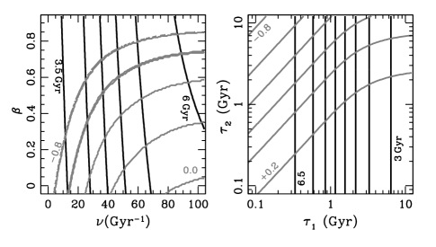
The extrema in metallicity are and . represents the timescale for the formation of the stellar component, whereas drives the metal enrichment. In this paper, we consider as free parameters , and the formation epoch, zFOR, allowing for a wide range of star formation histories with a decoupling between star formation, gas infall and outflows. As an example, Fig. 2 shows the relationship between star formation rate (assuming a delayed exponential law) and metallicity for three models. Note that the dotted line, corresponding to a balance between enrichment and infall, gives a metallicity distribution similar to the closed box model, producing an excess of stars at low metallicity. This so-called G-dwarf problem (see, e.g., Pagel, 1997) – is solved in this framework by a fast enrichment (short ) along with an extended period of infall (long ). To illustrate the validity of these models, we compare the age and metallicity distributions with a more detailed analysis based on standard prescriptions of chemical enrichment. These more detailed models describe the build up of the stellar populations and their metallicities by a process of gas infall/outflow – where the infall and outflow rates are controlled by free parameters – along with a Schmidt (1963) law to drive the transformation of gas into stars, and an additional parameter for the star formation efficiency that regulates the fraction of the gas component that is transformed into stars per unit time (see Ferreras & Silk, 2001; Ferreras et al., 2004, for details). In Fig. 3, contours of average stellar age (black lines) and metallicity (grey lines) are shown with respect to star formation efficiency () and outflow fraction () for the enrichment model (left) or with respect to the two timescales ( and ) for the phenomenological model used here (right). The formation epoch is fixed in both cases to . A mapping can be established between star formation efficiency () and our ; and also between outflow fraction () and our . We emphasize that the model presented here is meant to give a simple and clear representation of the formation of the stellar populations in disc galaxies.
4 Results
The models presented in the previous section are explored over a large range of parameters. We also include the effects of dust as a homogeneous screen. We describe this component as an additional fourth free parameter, choosing the colour excess, , from the Cardelli et al. (1989) extinction law. In order to obtain the most robust estimates of the best fit and uncertainty, we opt for a comprehensive search of parameter space. This is doable given the small number of parameters describing the star formation history. Furthermore, a parameter search algorithm has a very simple parallelisation scheme, so that we can run it efficiently on many processors. For a choice of the four parameters, the resulting star formation history is combined with the synthetic populations of Bruzual & Charlot (2003) to derive the six (five) broadband photometric colours available from the FDF (WHDF) data, generating a likelihood (via a standard statistic), that defines a probability distribution function for the three parameters under consideration. Out of the two families of models – corresponding to either a delayed exponential, or a model – we select for each galaxy the one that gives the lowest value of the . Although discriminating between these two prescriptions for the star formation history is beyond the capabilities of broadband photometry, we note that there is a slight preference towards the delayed exponential model, especially at low stellar mass. Roughly in 70% of the sample a delayed exponential model is preferred over a model. However, the trends in the average ages and metallicities are not affected by the choice. We note there is a 1:1 correspondence between the predicted age in both cases for populations younger than 3 Gyr, whereas delayed exponential models give ages Gyr younger than the models for older populations. The trend with metallicity is similar, with a 1:1 correspondence at solar/supersolar metallicities and offsets 0.2 dex more metal rich in the delayed exponential models. We derive from the likelihood the average mass-weighted age and metallicity, along with the uncertainties, quoted throughout this paper at the 69% level. For each galaxy, we run two grids of models (one for each choice of star formation rate), uniformly scaled over the following range of the parameters:
In addition, we impose a prior on the average stellar metallicity, using the local mass-metallicity relation of Gallazzi et al. (2005). We note that this prior is rather mild, given the large scatter of the distribution at fixed mass ( dex at ). The reason for applying this prior is based on the lack of a large number of independent metallicities in the synthetic models, along with the fact that broadband photometry alone – only extending out to rest-frame data in the band, given the redshift range – cannot impose strong constraints on the metallicities of unresolved stellar populations. This prior helps to ensure a correct age-metallicity discrimination in the analysis. The error bars on the estimates of stellar metallicity are around dex and the average age uncertainties . A comparison between the ages derived with and without the prior on metallicity gives a difference Gyr, without any systematic effect with respect to galaxy mass.
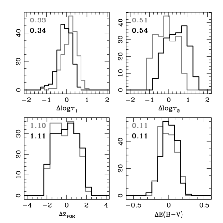
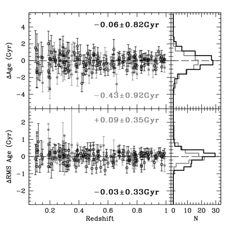
In order to confirm this point, we performed 200 simulations with the same redshift and signal-to-noise distribution as the original data, comparing the age and RMS of the age distribution. Fig. 4 shows the difference between the input and the recovered values for the average age (top) and the RMS of the age distribution (bottom). The simulations assume two different cases of stellar mass for the application of the prior: M⊙ (black) and M⊙ (grey). In either case, the recovered values do not show any systematic offset, with an accuracy of Gyr in average age and Gyr in the RMS of the age distribution. In Fig. 5 a similar comparison is made, in this case between the model parameters. The numbers in each panel give the RMS of the distributions of the (input output) values of the parameters for the simulations. Note that there is no systematic change in the values of the parameters, except for . In this case, as expected, the prior biases the values of metallicity towards lower metallicity for the M⊙ (grey) case, and towards higher metallicity at M⊙ (black). We note that our approach is quite conservative, as the prior for the simulations is blindly applied to all galaxies, irrespective of their input value of metallicity.
4.1 Model parameters
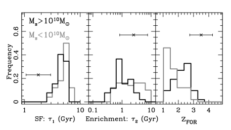
Hereafter, we present the results for the FDF/WHDF data. Fig. 6 shows the distribution of the two formation timescales and the formation epoch. The sample is split with respect to stellar mass, at the position of the median (M⊙). For reference, the median uncertainty (at the 68% level) is shown in each panel as a horizontal error bar. Note the difference between the distribution of low- and high-mass discs, especially in the enrichment timescale, and the formation epoch. The majority of low-mass discs (grey histograms) are fitted by longer timescales both in star formation () and enrichment (), along with later formation times. A large fraction (56%) of the massive galaxies (MM⊙) are better explained by very short enrichment timescales ( Gyr), in contrast with 28% for the low-mass subsample. Low values of both and would represent the efficient and fast buildup of the stellar populations expected in early-type galaxies (see, e.g., de la Rosa et al., 2011). In contrast, massive discs have more extended star formation timescales (reflecting a lower star formation efficiency or an extended infall), and short enrichment timescales (possibly caused by a lack of metal-rich outflows). The difference in the error bars for and is caused by the higher accuracy on the age estimates, with respect to metallicity.
| X | Redshift | Y | |||
|---|---|---|---|---|---|
| Range | zFOR | EB-V | |||
| Ms | All | ||||
| z | |||||
| z | |||||
| Mdyn | All | ||||
| z | |||||
| z | |||||
| Ms/M | All | ||||
| z | |||||
| z | |||||
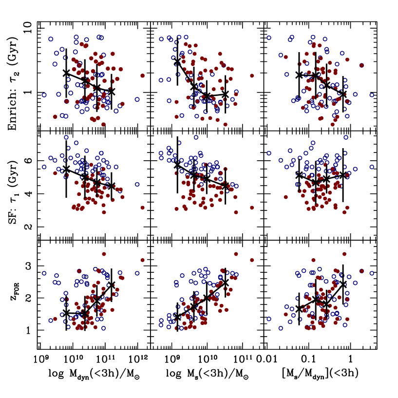
Fig. 7 shows the best fit parameters as a function of physical properties: dynamical mass (left), stellar mass (centre), or stellar-to-dynamical mass fraction (right). To avoid model-dependent extrapolations for the dark matter distribution, both dynamical and stellar masses are quoted within a fixed aperture of exponential scale lengths (roughly where all galaxies in the sample reach a flat circular velocity), i.e. the dynamical mass is given as M, where is the disc scale length. The scale lengths are derived from surface brightness fits to the ACS images (Böhm & Ziegler, 2007). The average fractional error for the sample explored in this paper is 20% in the disc scale length. Including the 0.087 dex error in (propagated from uncertainties in inclination and the fit of the rotation curve) results in an average error of dex. The stellar mass uncertainty – obtained from the PDF derived by the large volume of parameter space explored by the models – is dex. For a clearer interpretation of the trends, the individual data points are arranged into four bins. The binning is done at constant number of galaxies per bin, and the median and dispersion (RMS) are shown as crosses, and error bars, respectively. The individual data points are also coded with respect to redshift (red solid: ; open blue: ). Note that the parameters are correlated with stellar mass, with a clear downsizing trend with .
Tab. 1 gives the non-parametric correlations according to the Spearman test (see, e.g., Press et al., 1992) for all four free parameters explored by the models. Values close to () reflect a strong correlation (anticorrelation). The numbers in brackets underneath each case correspond to the expected value for a random distribution. It is obtained by a bootstrapping method, where 1000 realisations are created by randomly shuffling the data points 1000 times for each realisation. The quoted numbers (shown in brackets) give the 90th percentile of this randomly generated distribution of Spearman’s correlation coefficients. Hence, numbers smaller, in absolute number, to this figure would imply no correlation. Notice the strongest correlation for the parameters shown in Fig. 7 is found between stellar mass and formation epoch. The weak correlation between and Ms/Mdyn could be explained with the assumption that this fraction is an indicator of efficiency or gas outflows, hence, at large stellar masses, one should expect a fast, efficient buildup of metallicity (i.e. a short ), however, we emphasize that the level of correlation is at the border line, much weaker than any other trend with stellar mass. Regarding redshift, the strongest trend is with star formation/infall timescale (, middle panels), reflecting a more extended distribution of ages in the sample at low redshift, mostly due to the wider range of ages because of lookback time.
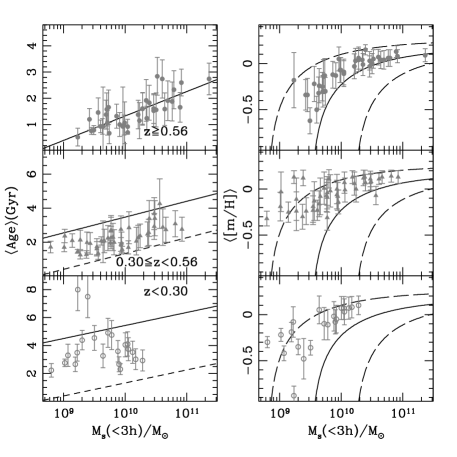
The trends of average age and metallicity with stellar mass are shown in Fig. 8, split into three redshift bins, that correspond to uniform steps of Gyr in lookback times between bins. Error bars are shown at the 68% confidence level. In the top-left panel of the figure, we fit the high redshift (z) subsample, creating copies of the same fit in the other two bins (dashed lines on the middle-left and bottom left panels), also showing a version shifted in age by the lookback time (solid lines). When taking into account the effect of lookback time, we find that the average ages are Gyr younger than the expectations from the fit at high redshift, reflecting the fact that passive evolution does not give a good representation to these galaxies. Although this could be interpreted as a lack of ”dynamical downsizing”, the sample is not large enough to constrain a change in slope of the correlation between age and stellar mass. As regards to metallicity, there is a trend towards the metal rich envelope of the local mass-metallicity relation. Note the present analysis, based on broadband photometry alone, mainly constrains stellar ages, whereas estimates of metallicity carry a large error bar (typically dex). Even though the local mass-metallicity relation is used as a mild prior in the analysis, we stress that the minimum values of are not significantly affected by the prior, with % of the sample having a reduced value .
4.2 The evolution of the Tully-Fisher relation
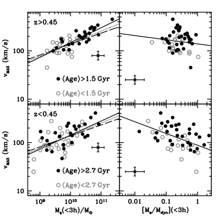
Fig. 9 shows the properties of the underlying stellar populations on a variation of the Tully-Fisher diagram (Tully & Fisher, 1977). The sample is split at the median redshift (top/bottom panels), and in each panel, black solid (grey open) circles represent disc galaxies with an average age older (younger) than the mean value within each redshift bin, as labelled. Typical () error bars are shown as reference. The panels on the left show a vs stellar mass Tully-Fisher relation. The usual downsizing relation between stellar mass and age is found. However, at fixed stellar mass, no significant segregation with respect to is evident. Old and young discs show a similar amount of scatter with respect to the best linear fit (solid line). The slope and intercept (see Tab. 2) are indistinguishable (as also found by, e.g. Miller et al., 2011, 2012, out to z1.7) with respect to the redshift subsample chosen (). The panels on the right show the maximum circular speed with respect to stellar-to-dynamical mass fraction, with a clear trend towards a faster for disc galaxies with a lower stellar mass fraction, as expected, since the stellar-to-total mass ratio decreases with increasing galaxy mass (see, e.g., Moster et al., 2010). At fixed mass fraction, the younger galaxies have slower rotation speeds. One can assume that the stellar-to-dynamical mass fraction controls the level of “baryon feedback” – mainly related to star formation in this sample. A tentative interpretation of the segregation with respect to age, at fixed , would be that older galaxies are preferentially assembled in higher density haloes, therefore having a higher circular speed.
4.3 The contribution of dust
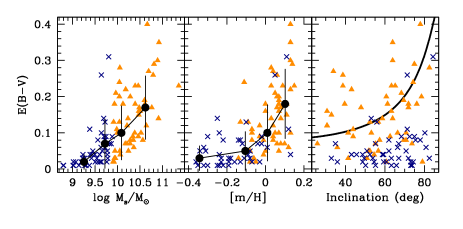
Fig. 10 shows the trend of dust reddening with respect to stellar mass, average metallicity or inclination. The sample is split at the median value of the stellar mass ( M⊙), with the orange triangles (blue crosses) corresponding to stellar masses above (below) this cut. The big solid dots with error bars in the left and middle panels give the median and RMS scatter of the complete sample, binned at fixed number of galaxies per bin. A prescription from Tully & Fouqué (1985) is included for reference, with and (solid line). A strong trend is found with respect to mass and metallicity, in good agreement with the observations of local discs (Tully et al., 1998). The last column of Tab. 1 indicates that stellar mass, and not dynamical mass, is the main mass observable correlated with colour excess. More subtle is the excess of more attenuated galaxies at higher inclinations for the more massive galaxies. Notice that our modelling does not impose any prior constraint on the colour excess, considering all values of in the analysis. The formalism of Tully & Fouqué (1985) is applicable for the massive disc subsample, whereas lower mass discs are not affected so strongly with respect to disc inclination.
| MM | ||
|---|---|---|
| Redshift | Ms,100 | |
| Range | M⊙ | |
| All | ||
| z | ||
| z | ||
4.4 Star formation rates (SFRs)
Ongoing star formation rates can be derived from emission line luminosities. In this paper, following Kennicutt (1992), we derive SFRs from the equivalent widths of [O II], and the -band luminosity, namely:
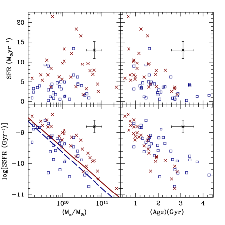
where is the dust extinction correction factor at the wavelength of Hα. Fig. 11 presents the SFRs (top) and specific SFRs (SSFR, defined as the SFR per unit stellar mass, bottom) with respect to either stellar mass (left) or average age (right). The sample is split with respect to redshift at the median value of the subsample comprising galaxies where SFRs could be determined (), with blue open squares (red crosses) corresponding to low (high) redshift. Only a subset of the full sample is presented here because the derivation of SFRs require estimates of [O II] luminosities. Characteristic error bars, at the level are shown for reference. A strong correlation is found between SSFR and age. In the bottom-left panel, the rates measured in our sample are compared with the general trend of star-forming galaxies from Brinchmann & Ellis (2000) at (solid line) and (dashed line).
5 Conclusions
By comparing optical to NIR photometry of a sample of disc galaxies at intermediate redshift, with a simple set of phenomenological one-zone models including chemical enrichment, we are able to explore the formation of these systems and the evolution of the Tully-Fisher relation. We find a correlation between the parameters that describe the star formation history and stellar mass. Dynamical mass provides equivalent, but weaker trends. The formation epoch is especially correlated with stellar mass, showing the usual downsizing trend, with the most massive discs forming around . The SF and enrichment timescales have weaker, but detectable correlations with stellar mass, towards shorter SF timescales ( Gyr), and fast enrichment times ( Gyr) for the most massive galaxies, reflecting a very efficient process for the build-up of metallicity in these systems. These are the typical enrichment timescales for the enrichment of massive early-type galaxies (see, e.g. Ferreras & Silk, 2001), however, our massive discs have longer SF timescales, resulting in an extended distribution of stellar ages. On the Tully-Fisher plane, age does not introduce a segregation at fixed circular speed, suggesting mild evolution of the Tully-Fisher relation with redshift.
We also present the model fits with respect to dynamical mass (measured within three scale lengths) and find a similar trend as with respect to stellar mass. However, the ratio of the two – an estimator of dark matter fraction, or feedback efficiency – seem not to correlate with the model parameters, reinforcing the idea that mass is the strongest, first order driver of the star formation histories of galaxies. Nevertheless, on the Tully-Fisher diagram (Fig. 9), at fixed , older galaxies have faster circular speeds, perhaps reflecting the fact that older discs would have formed in higher density halos, hence the higher . The difference is rather small, and a more detailed analysis – based on spectroscopic data with high SNR and accurate flux calibration – is needed to confirm this trend.
Our model includes dust as a free parameter, treated as a simple dust screen. Our findings agree independently with the formalism of Tully & Fouqué (1985) for the most massive discs (stellar mass ), with lower mass discs featuring no significant trend between colour excess and inclination.
Acknowledgments
AB thanks the Austrian Science foundation FWF for funding (project P23946-N16). The referee is warmly thanked for his/her useful comments and suggestions. The authors acknowledge the use of the UCL Legion High Performance Computing Facility (Legion@UCL), and associated support services, in the completion of this work.
References
- Bell & de Jong (2001) Bell, E. F., de Jong, R. S., 2001, ApJ, 550, 212
- Brinchmann & Ellis (2000) Brinchmann, J., Ellis, R. S., 2000, ApJ, 536, L77
- Bruzual (1983) Bruzual, G., 1983, ApJ, 273, 105
- Bruzual & Charlot (2003) Bruzual, G., Charlot, S., 2003, MNRAS, 344, 1000
- Böhm et al. (2004) Böhm, A., et al. 2004, A&A, 420, 97
- Böhm & Ziegler (2007) Böhm, A., Ziegler, B., 2007, ApJ, 668, 846
- Cardelli et al. (1989) Cardelli, J. A., Clayton, G. C., Mathis, J. S., 1989, ApJ, 345, 245
- Cimatti et al. (2006) Cimatti, A., Daddi, E. & Renzini, A., 2006, A&A, 453, L29
- Cowie et al. (1996) Cowie, L. L., Songaila, A., Hu, E. M., Cohen, J. G., 1996, AJ, 112, 839
- de la Rosa et al. (2011) de La Rosa, I. G., La Barbera, F., Ferreras, I., de Carvalho, R. R. 2011, MNRAS, 418 L74
- Dutton et al. (2007) Dutton, A. A., van den Bosch, F. C., Dekel, A., Courteau, S., 2007, ApJ, 654, 27
- Fernández-Lorenzo et al. (2009) Fernández-Lorenzo, M., Cepa, J., Bongiovanni, A., Castañeda, H., Pérez García, A. M., Lara-López, M. A., Pović, M., Sánchez-Portal, M., 2009, A&A, 496, 389
- Ferreras & Silk (2001) Ferreras, I. & Silk, J., 2001, ApJ, 557, 165
- Ferreras et al. (2004) Ferreras, I., Silk, J., Böhm, A. & Ziegler, B., 2004, MNRAS, 355, 64
- Flores et al. (2006) Flores, H., Hammer, F., Puech, M., Amram, P., Balkowski, C., 2006, A&A, 455, 107
- Gallazzi et al. (2005) Gallazzi, A., Charlot, S., Brinchmann, J,. White, S. D. M., Tremonti, C. A., 2005, MNRAS, 362, 41
- Giovanelli et al. (1997) Giovanelli, R., Haynes, M. P., da Costa, L. N., Freudling, W., Salzer, J. J., Wegner, G., 1997, ApJ, 477, L1
- Governato et al. (2009) Governato, F. et al., 2009, MNRAS, 398, 312
- Heidt et al. (2003) Heidt, J., et al. 2003, A&A, 398, 49
- Kauffmann et al. (2003) Kauffmann, G., et al., 2003, MNRAS, 341, 54
- Kennicutt (1992) Kennicutt, R. C., 1992, ApJ, 388, 310
- Khalatyan et al. (2008) Khalatyan, A., Cattaneo, A., Schramm, M., Gottlöber, S., Steinmetz, M., Wisotzki, L., 2008, MRAS, 387, 13
- Kodama et al. (2004) Kodama, T., et al., MNRAS, 350, 1005
- McGaugh et al. (2000) McGaugh, S. S., Schombert, J. M., Bothun, G. D., de Blok, W. J. G., 2000, ApJ, 533, L99
- McGaugh (2012) McGaugh, S. S., 2012, AJ, 143, 40
- Mathis et al. (2002) Mathis, H., Lemson, G., Springel, V., Kauffmann, G., White, S. D. M., Eldar, A., Dekel, A., 2002, MNRAS, 333, 739
- Metcalfe et al. (2001) Metcalfe, N., Shanks, T., Campos, A., McCracken, H. J., Fong, R., 2001, MNRAS, 323, 795
- Miller et al. (2011) Miller, S. H., Bundy, K., Sullivan, M., Ellis, R. S., Treu, T., 2011, ApJ, 741, 115
- Miller et al. (2012) Miller, S. H., Ellis, R. S., Sullivan, M., Bundy, K., Newman, A. B., Treu, T., 2012, ApJ, 753, 74
- Moster et al. (2010) Moster B. P., Somerville R. S., Maulbetsch C., van den Bosch F. C., Macciò A. V., Naab T., Oser L., 2010, ApJ, 710, 903
- Pagel (1997) Pagel, B. E. J., 1997, Nucleosynthesis and Chemical Evolution of Galaxies. Cambridge University Press, Cambridge
- Peng et al. (2002) Peng, C. Y., Ho, L. C., Impey, C. D., Rix, H.-W., 2002, AJ, 124, 266
- Pérez-González et al. (2008) Pérez-González, P. G., et al., 2008, ApJ, 675, 234
- Portinari & Sommer-Larsen (2007) Portinari, L., Sommer-Larsen, J., 2007, MNRAS, 375, 913
- Press et al. (1992) Press, W. H., Teukolsky, S. A., Vetterling, W. T., Flannery, B. P., 1992, Numerical Recipes in C (Cambridge Univ. Press)
- Puech et al. (2008) Puech, M. et al., 2008, A&A, 484, 173
- Rogers et al. (2010) Rogers, B., Ferreras, I., Pasquali, A., Bernardi, M., Lahav, O., Kaviraj, S., 2010, MNRAS, 405, 329
- Schlegel et al. (1998) Schlegel, D. J., Finkbeiner, D. P., Davis, M., 1998, ApJ, 500, 525
- Schmidt (1963) Schmidt, M., 1963, ApJ, 137, 758
- Tonini et al. (2011) Tonini, C., Maraston, C., Ziegler, B., Böhm, A., Thomas, D., Devriendt, J., Silk, J., 2011, MNRAS, 415, 811
- Tully & Fisher (1977) Tully, R. B., Fisher, J. R., 1977, A&A, 54, 661
- Tully & Fouqué (1985) Tully, B. & Fouqué, 1985, ApJS, 58, 67
- Tully et al. (1998) Tully, R. B., Pierce, M. J., Huang, J.-S., Saunders, W., Verheijen, M. A. W., Witchalls, P. L., 1998, AJ, 115, 2264
- van den Bosch et al. (2008) van den Bosch, F. C., et al. 2008, MNRAS, 387, 79
- Vogt et al. (1996) Vogt, N. P., Forbes, D. A., Phillips, A. C., Gronwall, C., Faber, S. M., Illingworth, G. D., Koo, D. C. 1996, ApJ, 465, L15
- Weiner et al. (2006) Weiner, B., et al. 2006, ApJ, 653, 1049
- Ziegler et al. (2002) Ziegler, B. L., et al. 2002, ApJ, 564, L69