Abstract: We wish to estimate conditional density using Gaussian Mixture Regression model with logistic weights and means depending on the covariate. We aim at selecting the number of components of this model as well as the other parameters by a penalized maximum likelihood approach. We provide a lower bound on penalty, proportional up to a logarithmic term to the dimension of each model, that ensures an oracle inequality for our estimator. Our theoretical analysis is supported by some numerical experiments.

Key-words: Conditional density estimation, Gaussian Mixture Regression, Model selection

Gaussian Mixture Regression model with logistic weights, a penalized maximum likelihood approach

Résumé : Nous souhaitons estimer une densité conditionelle à l’aide d’un modèle de mélange de régression gaussienne à poids logistiques et moyennes dépendant d’une covariable. L’objectif est de sélectionner le nombre de composantes dans le modèle ainsi que d’estimer les autres paramètres par une approche de type maximum de vraisemblance pénalisé. Nous proposons une borne inférieur sur la pénalité, proportionelle à un facteur logarithmique près, à la dimension de chaque modèle, qui assure l’existence d’une inégalité oracle pour notre estimateur. Notre analyse théorique est confirmée par des expériences numériques.

Mots-clés : Estimation de densité conditionnelle, Mélange de régression gaussienne, Sélection de modèles

Gaussian Mixture Regression model with logistic weights, a penalized maximum likelihood approach

1 Framework

In classical Gaussian mixture models, density is modeled by

$$s_{K,\upsilon,\Sigma,w}(y)=\sum_{k=1}^{K}\pi_{w,k}\Phi_{\upsilon_{k},\Sigma_{k}}(y),$$

where $K\in\mathbb{N}^{*}$ is the number of mixture components, $\Phi_{\upsilon,\Sigma}$ is the density of a Gaussian of mean $\upsilon$ and covariance matrix $\Sigma$,

$$\Phi_{\upsilon,\Sigma}(y)=\frac{1}{\sqrt{(2\pi)^{p}|\Sigma|}}e^{\frac{-1}{2}(y-\upsilon)^{\prime}\Sigma^{-1}(y-\upsilon)}$$

and mixture weights can always be defined from a $K$-tuple $(w_{1},\ldots,w_{K})$ with a logistic scheme:

$$\pi_{w,k}=\frac{e^{w_{k}}}{\sum_{k^{\prime}=1}^{K}e^{w_{k^{\prime}}}}.$$

In this article, we consider such a model in which mixture weights as well as means can depend on a covariate.

More precisely, we observe $n$ pairs of random variables $((X_{i},Y_{i}))_{1\leq i\leq n}$ where covariates $X_{i}$s are independent and $Y_{i}$s are independent conditionally to the $X_{i}$s. We want to estimate the conditional density $s_{0}(\cdot|x)$ with respect to the Lebesgue measure of $Y$ given $X$. We model this conditional density by a mixture of Gaussian regression with varying logistic weights

$$s_{K,\upsilon,\Sigma,w}(y|x)=\sum_{k=1}^{K}\pi_{w(x),k}\Phi_{\upsilon_{k}(x),\Sigma_{k}}(y),$$

where $(\upsilon_{1},\ldots,\upsilon_{K})$ and $(w_{1},\ldots,w_{K})$ are now $K$-tuples of functions chosen, respectively, in a set $\Upsilon_{K}$ and $W_{K}$. Our aim is then to estimate those functions $\upsilon_{k}$ and $w_{k}$, the covariance matrices $\Sigma_{k}$ as well as the number of classes $K$ so that the error between the estimated conditional density and the true conditional density is as small as possible.

The classical Gaussian mixture case has been much studied [18]. Nevertheless, theoretical properties of such model have been less considered. In a Bayesian framework, asymptotic properties of posterior distribution are obtained by Choi [7], Genovese and Wasserman [12], Van der Vaart and Wellner [19] when the true density is assumed to be a Gaussian mixture. AIC/BIC penalization scheme are often used to select a number of cluster (see Burnham and Anderson [4] for instance). Non asymptotic bounds are obtained by Maugis and Michel [16] even when the true density is not a Gaussian mixture. All these works rely heavily on a bracketing entropy analysis of the models, that will also be central in our analysis.

When there is a covariate, the most classical extension of this model is the Gaussian mixture regression, in which the means $\upsilon_{k}$ are now functions, is well studied as described inMcLachlan and Peel [18]. Models in which the proportions vary have been considered by Antoniadis et al. [1]. Using idea of Kolaczyk et al. [14], they have considered a model in which only proportion depend in a piecewise constant manner from the covariate. Their theoretical results are nevertheless obtained under the strong assumption they exactly know the Gaussian components. This assumption can be removed as shown by Cohen and Le Pennec [8]. Models in which both mixture weights and means depend on the covariate are considered by Ge and Jiang [11], but in a logistic regression mixture framework. They give conditions on the number of experts to obtain consistency of the posterior with logistic weights. Note that similar properties are studied by Lee [15] for neural networks.

Although natural, Gaussian mixture regression with varying logistic weights seems to be mentioned first by Jordan and Jacobs [13]. They provide an algorithm similar to ours, based on EM and IRLS, for hierarchical mixtures of experts but no theoretical analysis. Chamroukhi et al. [6] consider the case of piecewise polynomial regression model with affine logistic weights. In our setting, this corresponds to a specific choice for $\Upsilon_{K}$ and $W_{K}$: a collection of piecewise polynomial and a set of affine functions. They use a variation of the EM algorithm and a BIC criterion and provide numerical experiments to support the efficiency of their scheme. In this paper, we propose a slightly different penalty choice and prove non asymptotic bounds for the risk under very mild assumptions on $\Upsilon_{K}$ and $W_{K}$ that hold in their case.

2 A model selection approach

We will use a model selection approach and define some conditional density models $S_{m}$ by specifying sets of Gaussian regression mixture conditional densities through their number of classes $K$, a structure on the covariance matrices $\Sigma_{k}$ and two function sets $\Upsilon_{K}$ and $W_{K}$ to which belong respectively the $K$-tuple of means $(\upsilon_{1},\ldots,\upsilon_{K})$ and the $K$-tuple of logistic weights $(w_{1},\ldots,w_{K})$. Typically those sets are compact subsets of polynomial of low degree. Within such a conditional density set $S_{m}$, we estimate $s$ by the maximizer $\widehat{s}_{m}$ of the likelihood

$$\widehat{s}_{m}=\mathop{\text{argmax}}_{s_{K,\upsilon,\Sigma,w}\in S_{m}}\sum_{i=1}^{n}\ln s_{K,\upsilon,\Sigma,w}(Y_{i}|X_{i}),$$

or more precisely, to avoid any existence issue, by any $\eta$-minimizer of the -log-likelihood:

$$\sum_{i=1}^{n}-\ln\widehat{s}_{m}(Y_{i}|X_{i})\leq\min_{s_{K,\upsilon,\Sigma,w}\in S_{m}}\sum_{i=1}^{n}-\ln s_{K,\upsilon,\Sigma,w}(Y_{i}|X_{i})+\eta.$$

Assume now we have a collection $\{S_{m}\}_{m\in\mathcal{M}}$ of models, for instance with different number of classes $K$ or different maximum degree for the polynomials defining $\Upsilon_{K}$ and $W_{K}$, we should choose the best model within this collection. Using only the log-likelihood is not sufficient since this favors models with large complexity. To balance this issue, we will define a penalty $\mathop{\text{pen}}(m)$ and select the model $\widehat{m}$ that minimizes (or rather $\eta^{\prime}$-almost minimizes) the sum of the opposite of the log-likelihood and this penalty:

$$\sum_{k=1}^{K}-\ln\widehat{s}_{\widehat{m}}(Y_{i}|X_{i})+\mathop{\text{pen}}(\widehat{m})\leq\min_{m\in\mathcal{M}}\sum_{k=1}^{K}-\ln\widehat{s}_{m}(Y_{i}|X_{i})+\mathop{\text{pen}}(m)+\eta^{\prime}.$$

Our goal is now to define a penalty $\mathop{\text{pen}}(m)$ which ensures that the maximum likelihood estimate in the selected model performs almost as well as the maximum likelihood estimate in the best model. More precisely, we will prove that

$$\mathbb{E}\left[\mathrm{JKL}_{\rho}^{\otimes n}(s_{0},\widehat{s}_{\widehat{m}})\right]\leq C_{1}\inf_{m\in\mathcal{M}}\left(\inf_{s_{m}\in S_{m}}\mathrm{KL}^{\otimes n}(s_{0},s_{m})+\frac{\mathop{\text{pen}}(m)}{n}+\frac{\eta+\eta^{\prime}}{n}\right)+\frac{C_{2}}{n}$$

where $\mathrm{KL}^{\otimes n}$ is a tensorized Kullback-Leibler divergence, $\mathrm{JKL}_{\rho}^{\otimes n}$ a lower bound of this divergence with a $\mathop{\text{pen}}(m)$ chosen of the same order as the variance of the corresponding single model maximum likelihood estimate. In the next section, we specify all those divergences and explain the general framework proposed by Cohen and Pennec [9] for conditional density estimation. We will then explain how to use those results in our specific setting. The last section is dedicated to some numerical experiments conducted for sake of simplicity in the case where $X\in[0,1]$ and $Y\in\mathbb{R}$.

3 A general conditional density model selection theorem

We summarize in this section the main result of Cohen and Pennec [9] that will be our main tool to obtain the previous oracle inequality. In this work, the estimator loss is measured with a divergence $\mathrm{JKL}^{\otimes n}$ defined as a tensorized Kullback-Leibler divergence between the true density and a convex combination of the true density and the estimated one. Contrary to the true Kullback-Leibler divergence, to which it is closely related, it is bounded. This boundedness turns out to be crucial to control the loss of the penalized maximum likelihood estimate under mild assumptions on the complexity of the model and their collection.

Let $\mathrm{KL}$ be the classical Kullback-Leibler divergence, which measures a distance between two density functions. Since we work in a conditional density framework, we use a tensorized version of it. We define by $\mathrm{KL}^{\otimes n}$ the Kullback-Leibler tensorized divergence,

$$\mathrm{KL}^{\otimes n}(s,t)=\mathbb{E}\left[\frac{1}{n}\sum_{i=1}^{n}\mathrm{KL}(s(.|X_{i}),t(.|X_{i}))\right]$$

which appears naturally in this setting. Replacing $t$ by a convex combination between $s$ and $t$ yields the so-called Jensen-Kullback-Leibler tensorized divergence, denoted $\mathrm{JKL}_{\rho}^{\otimes n}$,

$$\mathrm{JKL}_{\rho}^{\otimes n}(s,t)=\mathbb{E}\left[\frac{1}{n}\sum_{i=1}^{n}\frac{1}{\rho}\mathrm{KL}(s(.|X_{i}),(1-\rho)s(.|X_{i})+\rho t(.|X_{i}))\right]$$

with $\rho\in]0;1[$. This loss is always bounded by $\frac{1}{\rho}\ln\frac{1}{1-\rho}$ but behaves as $\mathrm{KL}$ when $t$ is close to $s$. Furthermore $\mathrm{JKL}_{\rho}^{\otimes n}(s,t)\leq\mathrm{KL}_{\rho}^{\otimes n}(s,t)$. If we let $d^{2\otimes n}$ be the tensorized extension of the squared Hellinger distance $d^{2}$, Cohen and Pennec [9] prove that there is a constant $C_{\rho}$ such that $C_{\rho}d^{2\otimes n}(s,t)\leq\mathrm{JKL}_{\rho}^{\otimes n}(s,t)$.

To any model $S_{m}$, a set of conditional densities, we associate a complexity defined in term of a specific entropy, the bracketing entropy with respect to the root of $d^{2\otimes n}$. Recall that a bracket $[t^{-},t^{+}]$ is a pair of real functions such that $\forall(x,y)\in\mathcal{X}\times\mathcal{Y},t^{-}(x,y)\leq t^{+}(x,y)$ and a function $s$ is said to belong to the bracket $[t^{-},t^{+}]$ if $\forall(x,y)\in\mathcal{X}\times\mathcal{Y},t^{-}(x,y)\leq s(x,y)\leq t^{+}(x,y)$. The bracketing entropy $H_{[],d}(\delta,S)$ of a set $S$ is defined as the logarithm of the minimal number $N_{[],d}(\delta,S)$ of brackets $[t^{-},t^{+}]$ covering $S$, such that $d(t^{-},t^{+})\leq\delta$. Our main assumption on models is an upper bound of a Dudley type integral of these bracketing entropies:

Assumption (H)

For every model $S_{m}$ in the collection $\mathcal{S}$, there is a non-decreasing function $\phi_{m}$ such that $\delta\mapsto\frac{1}{\delta}\phi_{m}(\delta)$ is non-increasing on ]0,+$\infty$[ and for every $\sigma\in\mathbb{R}^{+}$,

$$\int_{0}^{\sigma}\sqrt{H_{[.],d^{\otimes n}}(\delta,S_{m})}d\delta\leq\phi_{m}(\sigma).$$

One need further to control the complexity of the collection as a whole through a coding type (Kraft) assumption.

Assumption (K)

There is a family $(x_{m})_{m\in\mathcal{M}}$ of non-negative numbers such that

$$\sum_{m\in\mathcal{M}}e^{-x_{m}}\leq\Xi<+\infty.$$

For technical reason, a separability assumption, always satisfied in the setting of this paper, is also required.

Assumption (Sep)

For every model $S_{m}$ in the collection $\mathcal{S}$, there exists some countable subset $S^{\prime}_{m}$ of $S_{m}$ and a set $\mathcal{Y^{\prime}}_{m}$ with $\lambda(\mathcal{Y}\backslash\mathcal{Y}^{\prime}_{m})=0$ such that for every $t$ in $S_{m}$, it exists some sequence $(t_{k})_{k\geq 1}$ of elements of $S^{\prime}_{m}$ such that for every $x$ and every $y\in\mathcal{Y}^{\prime}_{m},\ln(t_{k}(y|x))\xrightarrow[k\rightarrow+\infty]{}\ln(t(y|x))$.

The main result of Cohen and Pennec [9] is a condition on the penalty $\mathop{\text{pen}}(m)$ which ensures an oracle type inequality:

Theorem 1.

Assume we observe $(X_{i},Y_{i})$ with unknown conditional density $s_{0}$. Let $\mathcal{S}=(S_{m})_{m\in\mathcal{M}}$ an at most countable conditional density model collection. Assume assumptions (H), (Sep) and (K) hold. Let $\widehat{s}_{m}$ be a $\eta$ -log-likelihood minimizer in $S_{m}$

$$\sum_{i=1}^{n}-\ln(\widehat{s}_{m}(Y_{i}|X_{i}))\leq\inf_{s_{m}\in S_{m}}\left(\sum_{i=1}^{n}-\ln(s_{m}(Y_{i}|X_{i}))\right)+\eta$$

Then for any $\rho\in(0,1)$ and any $C_{1}>1$, there is a constant $\kappa_{0}$ depending only on $\rho$ and $C_{1}$ such that, as soon as for every index $m\in\mathcal{M}$,

$$pen(m)\geq\kappa(n\sigma^{2}_{m}+x_{m})$$

with $\kappa>\kappa_{0}$ and $\sigma_{m}$ the unique root of $\frac{1}{\sigma}\phi_{m}(\sigma)=\sqrt{n}\sigma$, the penalized likelihood estimate $\widehat{s}_{\widehat{m}}$ with $\widehat{m}$ such that

$$\sum_{i=1}^{n}-\ln(\widehat{s}_{\widehat{m}}(Y_{i}|X_{i}))+pen(\widehat{m})\leq\inf_{m\in\mathcal{M}}\left(\sum_{i=1}^{n}-\ln(\widehat{s}_{m}(Y_{i}|X_{i}))+pen(m)\right)+\eta^{\prime}$$

satisfies

$$\mathbb{E}\left[\mathrm{JKL}_{\rho}^{\otimes n}(s_{0},\widehat{s}_{\widehat{m}})\right]$$

$$\qquad\quad\leq C_{1}\inf_{m\in\mathcal{M}}\left(\inf_{s_{m}\in S_{m}}\mathrm{KL}_{\lambda}^{\otimes n}(s_{0},s_{m})+\frac{pen(m)}{n}\right)+C_{1}\frac{\kappa_{0}\Xi+\eta+\eta^{\prime}}{n}.$$

The name oracle type inequality means that the right-hand side is a proxy for the estimation risk of the best model within the collection. The term $\inf_{s_{m}\in S_{m}}\mathrm{KL}_{\lambda}^{\otimes n}(s_{0},s_{m})$ is a typical bias term while $\frac{pen(m)}{n}$ plays the role of the variance term. We have three sources of loss here: the constant $C_{1}$ can not be taken equal to $1$, we use a different divergence on the left and on the right and $\frac{pen(m)}{n}$ is not directly related to the variance. The first issue is often considered as minor while the second one turns out to be classical in density estimation results. Whenever $pen(m)$ can be chosen approximately proportional to the dimension $D_{m}$ of the model, which will be the case in our setting, $\frac{pen(m)}{n}$ is approximately proportional to $D_{m}/n$, which is the asymptotic variance in the parametric case. The right-hand side matches nevertheless the best known bound obtained for a single model within such a general framework.

In the next section, we show how to apply this result in our Gaussian mixture setting and prove that the penalty can be chosen roughly proportional to the intrinsic dimension of the model, and thus of the order of the variance.

4 Spatial Gaussian regression mixture estimation theorem

As explained in introduction, we are looking for conditional densities of type

$$s_{K,\upsilon,\Sigma,w}(y|x)=\sum_{k=1}^{K}\pi_{w,k}(x)\Phi_{\upsilon_{k}(x),\Sigma_{k}}(y),$$

where $K\in\mathbb{N}^{*}$ is the number of mixture components, $\Phi_{\upsilon,\Sigma}$ is the density of a Gaussian of mean $\upsilon$ and covariance matrix $\Sigma$, $\upsilon_{k}$ is a function specifying the mean given $x$ of the $k$-th component while $\Sigma_{k}$ is its covariance matrix and the mixture weights $\pi_{w,k}$ are defined from a collection of $K$ functions $w_{1},\ldots,w_{K}$ by a logistic scheme:

$$\pi_{w,k}(x)=\frac{e^{w_{k}(x)}}{\sum_{k^{\prime}=1}^{K}e^{w_{k^{\prime}}(x)}}.$$

For sake of simplicity, we will assume that the covariate $X$ belongs to an hypercube so that $\mathcal{X}=[0;1]^{d}$.

We will estimate those conditional densities by conditional densities belonging to some model $S_{m}$ defined by

$$S_{m}= \bigg{\{}(x,y)\mapsto\sum_{k=1}^{K}\pi_{w,k}(x)\Phi_{\upsilon_{k}(x),\Sigma_{k}}(y)\big{|}(w_{1},\ldots,w_{K})\in W_{K},(\upsilon_{1},\ldots,\upsilon_{K})\in\Upsilon_{K},$$

$$(\Sigma_{1},\ldots,\Sigma_{K})\in V_{K}\bigg{\}}$$

where $W_{K}$ is a compact set of $K$-tuples of functions from $\mathcal{X}$ to $\mathbb{R}$, $\Upsilon_{K}$ a compact set of $K$-tuples of functions from $\mathcal{X}$ to $\mathbb{R}^{p}$ and $V_{K}$ a compact set of $K$-tuples of covariance matrix of size $p\times p$. Before describing more precisely those sets, we recall that $S_{m}$ will be taken in a model collection $\mathcal{S}=(S_{m})_{m}$, where $m$ specifies a choice for each of those parameters. The number of components $K$ can be chosen arbitrarily in $\mathbb{N}^{*}$, but will in practice and in our theoretical example be chosen smaller than an arbitrary $K_{\max}$, which may depend on the sample size $n$. The sets $W_{K}$ and $\Upsilon_{K}$ will be typically chosen as a tensor product of a same compact set of moderate dimension, for instance a set of polynomial of degree smaller than respectively $d_{W}$ and $d_{\Upsilon}$ whose coefficients are smaller in absolute values than respectively $T_{W}$ and $T_{\Upsilon}$. The structure of the set $V_{K}$ depends on the noise model chosen: we can assume, for instance, it is common to all regressions, that they share a similar volume or diagonalization matrix or they are all different. More precisely, we decompose any covariance matrix $\Sigma$ into $LDAD^{\prime}$, where $L=|\Sigma|^{1/p}$ is a positive scalar corresponding to the volume, $D$ is the matrix of eigenvectors of $\Sigma$ and $A$ the diagonal matrix of normalized eigenvalues of $\Sigma$. Let $L_{-},L_{+}$ be positive values and $\lambda_{-},\lambda_{+}$ real values. We define the set $\mathcal{A}(\lambda_{-},\lambda_{+})$ of diagonal matrices $A$ such that $|A|=1$ and $\forall i\in\{1,\ldots,p\},\lambda_{-}\leq A_{i,i}\leq\lambda_{+}$. A set $V_{K}$ is defined by

$$V_{K}= \left\{(L_{1}D_{1}A_{1}D_{1}^{\prime},\ldots,L_{K}D_{K}A_{K}D_{K}^{\prime})|\forall k,L_{-}\leq L_{k}\leq L_{+},D_{k}\in SO(p),\right.$$

$$\left.A_{k}\in\mathcal{A}(\lambda_{-},\lambda_{+})\right\}$$

Those sets $V_{K}$ correspond to the classical covariance matrix sets described by Celeux and Govaert [5].

We will bound the complexity term $n\sigma_{m}^{2}$ in term of the dimension of $S_{m}$: we prove that those two terms are roughly proportional. The set $V_{K}$ is a parametric set and thus $\dim(V_{K})$ is easily defined as the dimension of its parameter set. Defining the dimension of $W_{K}$ and $\Upsilon_{K}$ is more interesting. We rely on an entropy type definition of the dimension. For any $K$-tuples of functions $(s_{1},\ldots,s_{K})$ and $(t_{1},\ldots,t_{K})$, we let

$$d_{\|\sup\|_{\infty}}\left((s_{1},\ldots,s_{K}),(t_{1},\ldots,t_{K})\right)=\sup_{x\in\mathcal{X}}\sup_{1\leq k\leq K}|s_{k}(x)-t_{k}(x)|$$

and define the dimension $\dim(F_{K})$ of a set $F_{K}$ of such $K$-tuples as the smallest $D$ such that there is a $C$ satisfying

$$H_{d_{\|\sup\|_{\infty}}}(\sigma,F_{K})\leq D\left(C+\ln\frac{1}{\sigma}\right).$$

Using the following proposition of Cohen and Pennec [9], we can easily verify that Assumption (H) is satisfied.

Proposition 1.

If for any $\delta\in[0;\sqrt{2}],H_{[.],d^{\otimes n}}(\delta,S_{m})\leq D_{m}(C_{m}+\ln(\frac{1}{\delta}))$, then the function $\phi_{m}(\sigma)=\sigma\sqrt{D_{m}}\left(\sqrt{C_{m}}+\sqrt{\pi}+\sqrt{\ln(\frac{1}{\sigma\wedge 1})}\right)$ satisfies assumption (H). Furthermore, the unique root $\sigma_{m}$ of $\frac{1}{\sigma}\phi_{m}(\sigma)=\sqrt{n}\sigma$ satisfies

$$n\sigma_{m}^{2}\leq D_{m}\left(2(\sqrt{C_{m}}+\sqrt{\pi})^{2}+\left(\ln\frac{n}{(\sqrt{C_{m}}+\sqrt{\pi})^{2}D_{m}}\right)_{+}\right).$$

We show in Appendix that if

$$H_{d_{\|\sup\|_{\infty}}}(\sigma,W_{K})\leq\dim(W_{K})\left(C_{W_{K}}+\ln\frac{1}{\sigma}\right)$$

and

$$H_{\max_{k}\sup_{x}\|\|_{2}}(\sigma,\Upsilon_{K})\leq\dim(\Upsilon_{K})\left(C_{\Upsilon_{K}}+\ln\frac{1}{\sigma}\right)$$

then, if $n\geq 1$, the complexity of the corresponding model $S_{m}$ satisfies

$$n\sigma_{m}^{2} \leq D_{m}\left(2(\sqrt{C_{m}}+\sqrt{\pi})^{2}+\left(\ln\frac{n}{(\sqrt{C_{m}}+\sqrt{\pi})^{2}D_{m}}\right)_{+}\right)$$

$$\leq D_{m}\left(2(\sqrt{C_{m}}+\sqrt{\pi})^{2}+\ln(n)\right)$$

$$\leq D_{m}(C^{\prime}_{m}+\ln(n))$$

with $C^{\prime}_{m}$ that depends only on the constants defining $V_{K}$ and the constants $C_{W_{K}}$ and $C_{\Upsilon_{K}}$. In order to obtain the same constant $C^{\prime}_{m}$ for all models, we impose that the dimension bound holds with the same constants for all models:

Assumption (DIM)

There exist two constants $C_{W}$ and $C_{\Upsilon}$ such that, for every model $S_{m}$ in the collection $\mathcal{S}$,

$$H_{\max_{k}\|\|_{\infty}}(\sigma,W_{K})\leq\dim(W_{K})\left(C_{W}+\ln\frac{1}{\sigma}\right).$$

and

$$H_{\max_{k}\sup_{x}\|\|_{2}}(\sigma,\Upsilon_{K})\leq\dim(\Upsilon_{K})\left(C_{\Upsilon}+\ln\frac{1}{\sigma}\right)$$

We can now state our main result:

Theorem 2.

For any collection of Gaussian regression mixtures satisfying (K) and (DIM), there is a constant $C$ such that for any $\rho\in(0,1)$ and any $C_{1}>1$, there is a constant $\kappa_{0}$ depending only on $\rho$ and $C_{1}$ such that, as soon as for every index $m\in\mathcal{M}$, $pen(m)=\kappa((C+\ln n)\dim(S_{m})+x_{m})$ with $\kappa>\kappa_{0}$, the penalized likelihood estimate $\widehat{s}_{\widehat{m}}$ with $\widehat{m}$ such that

$$\sum_{i=1}^{n}-\ln(\widehat{s}_{\widehat{m}}(Y_{i}|X_{i}))+pen(\widehat{m})\leq\inf_{m\in\mathcal{M}}\left(\sum_{i=1}^{n}-\ln(\widehat{s}_{m}(Y_{i}|X_{i}))+pen(m)\right)+\eta^{\prime}$$

satisfies

$$\mathbb{E}\left[\mathrm{JKL}_{\rho}^{\otimes n}(s_{0},\widehat{s}_{\widehat{m}})\right]$$

$$\qquad\quad\leq C_{1}\inf_{m\in\mathcal{M}}\left(\inf_{s_{m}\in S_{m}}\mathrm{KL}_{\lambda}^{\otimes n}(s_{0},s_{m})+\frac{\mathop{\text{pen}}(m)}{n}+\frac{\kappa_{0}\Xi+\eta+\eta^{\prime}}{n}\right).$$

In the previous theorem, the assumption on $\mathop{\text{pen}}(m)$ could be replaced by the milder one

$$\mathop{\text{pen}}(m)\geq\kappa\left(2D_{m}C^{2}+D_{m}\left(\ln\frac{n}{C^{2}D_{m}}\right)_{+}+x_{m}\right).$$

To minimize arbitrariness, $x_{m}$ should be chosen such that $\frac{2\kappa x_{m}}{\mathop{\text{pen}}(m)}$ is as small as possible. Notice that the constant $C$ only depends on the model collection parameters, for instance on the maximal number of components $K_{\max}$. As often in model selection, the collection may be chosen according to to the sample size $n$. If the constant $C^{\prime}$ grows no faster than $\ln(n)$, the penalty shape can be kept intact and a similar result holds uniformly in $n$ up to a slightly larger $\kappa_{0}$. For instance, as $K_{\max}$ only appears in $C$ through a logarithmic term, $K_{\max}$ may grow as a power of the sample size.

We postpone the proof of this theorem to the Appendix and focus on Assumption (DIM). This assumption can often be verified when the functions sets $W_{K}$ and $\Upsilon_{K}$ are defined as images of a finite dimensional compact subset of parameters when $X\in[0,1]^{d}$. For example, those sets can be defined as linear combination of a finite set of bounded functions whose coefficients belong to a compact set. We study here the case of linear combination of the first elements of a polynomial basis but similar results hold, up to some modification on the coefficient sets, for many other choices (first elements of a Fourier, spline or wavelet basis, elements of an arbitrary bounded dictionary…)

Let $d_{W}$ and $d_{\Upsilon}$ be two integers and $T_{W}$ and $T_{\Upsilon}$ some positive numbers. We define

$$W =\left\{w:[0;1]^{d}\rightarrow\mathbb{R}|w(x)=\sum_{|r|=0}^{d_{W}}\alpha_{r}x^{r}\mbox{ and }\|\alpha\|_{\infty}\leq T_{W}\right\}$$

$$\Upsilon =\left\{\upsilon:[0;1]^{d}\rightarrow\mathbb{R}^{p}\Big{|}\forall j\in\{1,\ldots,p\},\forall x,\upsilon_{j}(x)=\sum_{|r|=0}^{d_{\Upsilon}}\alpha_{r}^{(j)}x^{r}\mbox{ and }\|\alpha\|_{\infty}\leq T_{\Upsilon}\right\}$$

Let $W_{K}=\{0\}\times W^{K-1}$ and $\Upsilon_{K}=\Upsilon^{K}$.

We prove in Appendix that

Lemma 1.

$W_{K}$ and $\Upsilon_{K}$ satisfy assumption (DIM), with $C_{W}=\ln\left(\sqrt{2}+T_{W}\binom{d_{W}+d}{d}\right)$ and $C_{\Upsilon}=\ln\left(\sqrt{2}+\sqrt{p}\binom{d_{\Upsilon}+d}{d}T_{\Upsilon}\right)$, not depending on $K$.

To apply Theorem 2, it remains to describe a collection $(S_{m})$ and a suitable choice for $(x_{m})$. Assume, for instance, that the models in our collection are defined by an arbitrary maximal number of components $K_{\max}$, a common free structure for the covariance matrix $K$-tuple and a common maximal degree for the sets $W_{K}$ and $\Upsilon_{K}$, then one can verify that $\dim(S_{m})=(K-1+Kp)\binom{d_{W}+d}{d}+Kp\frac{p+1}{2}$ and that the weight family $(x_{m}=K)$ satisfy Assumption (K) with $\Xi\leq 1/(e-1)$. Theorem 2 yields then an oracle inequality with $\mathop{\text{pen}}(m)=\kappa\left((C+\ln(n))\dim(S_{m})+x_{m}\right)$. Note that as $x_{m}\ll(C+\ln(n))\dim(S_{m})$, one can obtain a similar oracle inequality with $\mathop{\text{pen}}(m)=\kappa(C+\ln(n))\dim(S_{m})$ for a slightly larger $\kappa$. Finally, as explained in the proof, choosing a covariance structure from the finite collection of Celeux and Govaert [5] or choosing the maximal degree for the sets $W_{K}$ and $\Upsilon_{K}$ among a finite family can be obtained with the same penalty but with a larger constant $\Xi$ in Assumption (K).

5 Numerical scheme and numerical experiment

We illustrate our theoretical result in a setting similar to the one considered by Chamroukhi et al. [6]. We observe $n$ pairs $(X_{i},Y_{i})$ with $X_{i}\in[0,1]$ and $Y_{i}\in\mathbb{R}$ and look for the best estimate of the conditional density $s_{0}(y|x)$ that can be written

$$s_{K,\upsilon,\Sigma,w}(y|x)=\sum_{k=1}^{K}\pi_{w,k}(x)\Phi_{\upsilon_{k}(x),\Sigma_{k}}(y),$$

with $w\in W_{K}$ and $\upsilon\in\Upsilon_{K}$. We consider the simple case where $W_{K}$ and $\Upsilon_{K}$ comprise linear functions. We do not impose any structure on the covariance matrices. Our aim is to estimate the best number of components $K$, as well as the model parameters. As described with more details later, we use an EM type algorithm to estimate the model parameters for each $K$ and select one using the penalized approach described previously.

(a) 2 000 data points of example P

(b) 2 000 data points of example NP

Figure 1: Typical realizations

In our numerical experiment, we consider two different examples: one in which true conditional density belongs to one of our models, a parametric case, and one in which this is not true, a non parametric case. In the first situation, we expect to perform almost as well as the maximum likelihood estimation in the true model. In the second situation, we expect our algorithm to automatically balance the model bias and its variance. More precisely, we let

$$s_{0}(y|x)=\frac{1}{1+\exp(15x-7)}\Phi_{-15x+8,0.3}(y)+\frac{\exp(15x-7)}{1+\exp(15x-7)}\Phi_{0.4x+0.6,0.4}(y)$$

in the first example, denoted example P, and

$$s_{0}(y|x)=\frac{1}{1+\exp(15x-7)}\Phi_{15x^{2}-22x+7.4,0.3}(y)+\frac{\exp(15x-7)}{1+\exp(15x-7)}\Phi_{-0.4x^{2},0.4}(y)$$

in the second example, denoted example NP. For both experiments, we let $X$ be uniformly distributed over $[0,1]$. Figure 1 shows a typical realization for both examples.

As often in model selection approach, the first step is to compute the maximum likelihood estimate for each number of components $K$. To this purpose, we use a numerical scheme based on the EM algorithm [10] similar to the one used by Chamroukhi et al. [6]. The only difference with a classical EM is in the Maximization step since there is no closed formula for the weights optimization. We use instead a Newton type algorithm. Note that we only perform a few Newton steps (5 at most) and ensures that the likelihood does not decrease. We have noticed that there is no need to fully optimize at each step: we did not observe a better convergence and the algorithmic cost is high. We denote from now on this algorithm Newton-EM. Figure 2 illustrates the fast convergence of this algorithm towards a local maximum of the likelihood.

Figure 2: Increase of the Log-likelihood of the estimated density at each step of our iterative Newton-EM algorithm in the example NP with 3 components and 2 000 data points.

Notice that the lower bound on the variance required in our theorem appears to be necessary in practice. It avoids the spurious local maximizer issue of EM algorithm, in which a class degenerates to a minimal number of points allowing a perfect Gaussian regression fit. We use a lower bound of $\frac{10}{n}$. Biernacki and Castellan [3] provide a more precise data-driven bound: $\frac{\min_{1\leq i<j\leq n}(Y_{i}-Y_{j})^{2}}{2\chi^{2}_{n-2K+1}((1-\alpha)^{1/K})}$, with $\chi^{2}_{n-2K+1}$ the chi-squared quantile function, which is of the same order as $\frac{1}{n}$ in our case. In practice, the constant $10$ gave good results.

An even more important issue with EM algorithms is initialization, since the local minimizer obtained depends heavily on it. We observe that, while the weights $w$ do not require a special care and can be simply initialized uniformly equal to $0$, the means require much more attention in order to obtain a good minimizer. We propose an initialization strategy which can be seen as an extension of a Quick-EM scheme with random initialization.

We draw randomly $K$ lines, each defined as the line going through two points $(X_{i},Y_{i})$ drawn at random among the observations. We perform then a K-means clustering using the distance along the $Y$ axis. Our Newton-EM algorithm is initialized by the regression parameters as well as the empirical variance on each of the $K$ clusters. We perform then $3$ steps of our minimization algorithm and keep among $50$ trials the one with the largest likelihood. This winner is used as the initialization of a final Newton-EM algorithm using 10 steps.

We consider two other strategies: a naive one in which the initial lines chosen at random and a common variance are used directly to initialize the Newton-EM algorithm and a clever one in which observations are first normalized in order to have a similar variance along both the $X$ and the $Y$ axis, a K-means on both $X$ and $Y$ with $5$ times the number of components is then performed and the initial lines are drawn among the regression lines of the resulting cluster comprising more than $2$ points.

The complexity of those procedures differs and as stressed by Celeux and Govaert [5] the fairest comparison is to perform them for the same amount of time (5 seconds, 30 seconds, 1 minute…) and compare the obtained likelihoods. The difference between the 3 strategies is not dramatic: they yield very similar likelihoods. We nevertheless observe that the naive strategy has an important dispersion and fails sometime to give a satisfactory answer. Comparison between the clever strategy and the regular one is more complex since the difference is much smaller. Following Celeux and Govaert [5], we have chosen the regular one which corresponds to more random initializations and thus may explores more local maxima.

Once the parameters’ estimates have been computed for each $K$, we select the model that minimizes

$$\sum_{i=1}^{n}-\ln(\widehat{s}_{m}(Y_{i}|X_{i}))+\mathop{\text{pen}}(m)$$

with $\mathop{\text{pen}}(m)=\kappa\dim(S_{m})$. Note that our theorem ensures that there exists a $\kappa$ large enough for which the estimate has good properties, but does not give an explicit value for $\kappa$. In practice, $\kappa$ has to be chosen. The two most classical choices are $\kappa=1$ and $\kappa=\frac{\ln n}{2}$ which correspond to the AIC and BIC approach, motivated by asymptotic arguments. We have used here the slope heuristic proposed by Birgé and Massart and described for instance in Baudry et al. [2]. It consists in representing the dimension of the selected model according to $\kappa$ (fig 3), and finding $\hat{\kappa}$ such that if $\kappa<\hat{\kappa}$, the dimension of the selected model is large, and reasonable otherwise. The slope heuristic prescribes then the use of $\kappa=2\hat{\kappa}$. In both examples, we have noticed that the sample’s size had no significant influence on the choice of $\kappa$, and that very often 1 was in the range of possible values indicated by the slope heuristic. According to this observation, we have chosen in both examples $\kappa=1$.

(a) Example P with 2 000 points

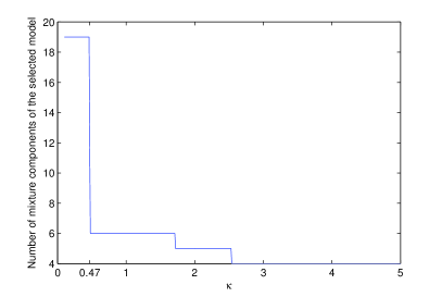
(b) Example NP with 2 000 points

Figure 3: Slope heuristic: plot of the selected model dimension with respect to the penalty coefficient $\kappa$. In both examples, $\widehat{\kappa}$ is of order $1/2$.

We measure performances in term of tensorized Kullback-Leibler distance. Since there is no known formula for tensorized Kullback-Leibler distance in the case of Gaussian mixtures, and since we know the true density, we evaluate the distance using Monte Carlo method. The variability of this randomized evaluation has been verified to be negligible in practice.

For several numbers of mixture components and for the selected K, we draw in figure 4 the box plots and the mean of tensorized Kullback-Leibler distance over $55$ trials. The first observation is that the mean of tensorized Kullback-Leibler distance between the penalized estimator $\hat{s}_{\hat{K}}$ and $s_{0}$ is smaller than the mean of tensorized Kullback-Leibler distance between $\hat{s}_{K}$ ans $s_{0}$ over $K\in\{1,\ldots,20\}$. This is in line with the oracle type inequality of Theorem 2. Our numerical results hint that our theoretical analysis may be pessimistic. A close inspection show that the bias-variance trade-off differs between the two examples. Indeed, since in the first one the true density belongs to the model, the best choice is $K=2$ even for small $n$. As shown on the histogram of Figure 5, this is almost always the model chosen by our algorithm. Observe also that the mean of Kullback-Leibler distance seems to behave like $\frac{\dim(S_{m})}{2n}$ (shown by a dotted line). This is indeed the expected behavior when the true model belongs to a nested collection and corresponds to the classical AIC heuristic. In the second example, the true model does not belong to the collection. The best choice for $K$ should thus balance a model approximation error and a variance one. We observe in Figure 5 such a behavior: the larger $n$ the more complex the model and thus $K$. Note that the slope of the mean error seems also to grow like $\frac{\dim(S_{m})}{2n}$ even though there is no theoretical guarantee of such a behavior.

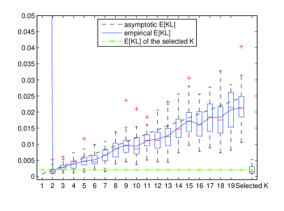
(a) Example P with 2 000 data points

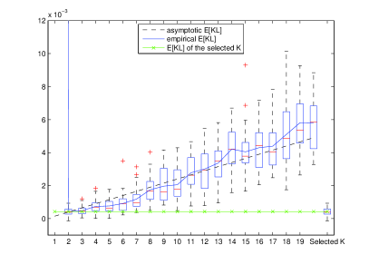
(b) Example P with 10 000 data points

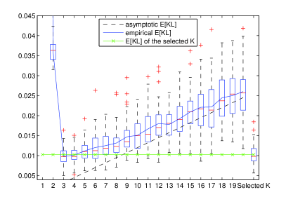
(c) Example NP with 2 000 data points

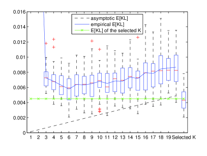
(d) Example NP with 10 000 data points

Figure 4: Box-plot of the Kullback-Leibler distance according to the number of mixture components. On each graph, the right-most box-plot shows this Kullback-Leibler distance for the penalized estimator $\hat{s}_{\widehat{K}}$

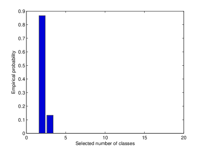
(a) Example P with 2 000 data points

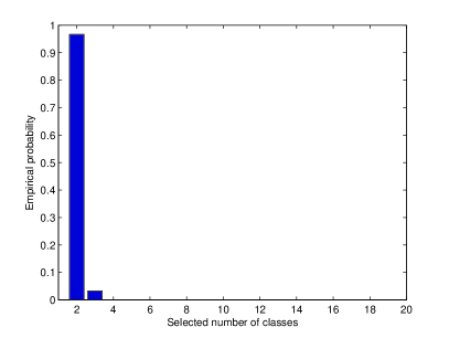
(b) Example P with 10 000 data points

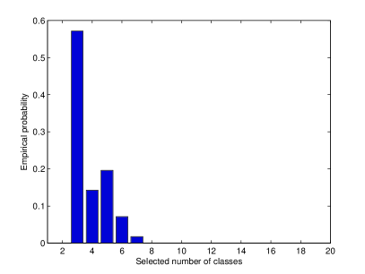
(c) Example NP with 2 000 data points

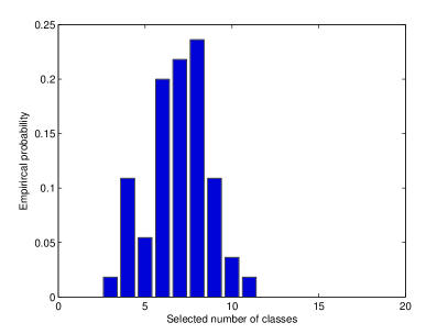
(d) Example NP with 10 000 data points

Figure 5: Histograms of the selected K

Figure 6 shows the error decay when the sample size $n$ grows. As expected in the parametric case, example P, we observe the decay in $t/n$ predicted in the theory, with $t$ some constant. The rate in the second case appears to be slower. Indeed, as the true conditional density does not belong to any model, the selected models are more and more complex when $n$ grows which slows the error decay. In our theoretical analysis, this can already be seen in the decay of the variance term of the oracle inequality. Indeed, if we let $m_{0}(n)$ be the optimal oracle model, the one minimizing the right-hand side of the oracle inequality, the variance term is of order $\frac{D_{m_{0}(n)}}{n}$ which is larger than $\frac{1}{n}$ as soon as $D_{m_{0}(n)}\to+\infty$. It is well known that the decay depends on the regularity of the true conditional density. Providing a minimax analysis of the proposed estimator, as have done Maugis and Michel [17], would be interesting but is beyond the scope of this paper.

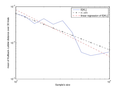
(a) Example P. The slope of the free regression line is $\simeq-1,3$

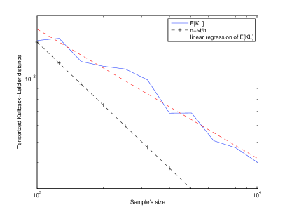
(b) Example NP. The slope of the regression line is $\simeq-0,6$.

Figure 6: Kullback-Leibler distance between the true density and the computed density using $(X_{i},Y_{i})_{i\leq N}$ with respect to the sample size, represented in a log-log scale. For each graph, we added a free linear least-square regression and one with slope $-1$ to stress the two different behavior.

Appendix A Proof of Theorem 2

In this section, an overview of the proof of the model selection theorem, applied to our Gaussian regression mixture, is given. B is dedicated to the example with polynomial means and weights. The constants in the Assumption (DIM) and the theorem are specified. Then, in C, we provide more details on the proofs and lemmas used in the first section.

We will show that Assumption (DIM) ensures that for all $\delta\in[0;\sqrt{2}],$ $H_{[.],d^{\otimes n}}(\delta,S_{m})\leq D_{m}(C_{m}+\ln(\frac{1}{\delta}))$ with a common $C_{m}$. If this happens, Proposition 1 yields the results. In other words, if we can control models’ bracketing entropy with a uniform constant $\mathfrak{C}$, we get a suitable bound on the complexity. This result will be obtain by first decomposing the entropy term between the weights and the Gaussian mixtures. Therefore we use the following distance over conditional densities:

$$\underset{x}{\sup}\,d_{y}(s,t)=\underset{x\in\mathcal{X}}{\sup}\,\left(\int_{y}\left(\sqrt{s(y|x)}-\sqrt{t(y|x)}\right)^{2}dy\right)^{\frac{1}{2}}.$$

Notice that $d^{2\otimes n}(s,t)\leq\sup_{x}d_{y}^{2}(s,t)$.

For all weights $\pi$ and $\pi^{\prime}$, we define

$$\underset{x}{\sup}\,d_{k}(\pi,\pi^{\prime})=\underset{x\in\mathcal{X}}{\sup}\,\left(\sum_{k=1}^{K}\left(\sqrt{\pi_{k}(x)}-\sqrt{\pi^{\prime}_{k}(x)}\right)^{2}\right)^{\frac{1}{2}}.$$

Finally, for all densities $s$ and $t$ over $\mathcal{Y}$, depending on $x$, we set

$$\underset{x}{\sup}\,\underset{k}{\max}\,d_{y}(s,t) =\underset{x\in\mathcal{X}}{\sup}\,\underset{1\leq k\leq K}{\max}\,d_{y}(s_{k}(x,.),t_{k}(x,.))$$

$$=\underset{x\in\mathcal{X}}{\sup}\,\underset{1\leq k\leq K}{\max}\,\left(\int_{y}\left(\sqrt{s_{k}(x,y)}-\sqrt{t_{k}(x,y)}\right)^{2}dy\right)^{\frac{1}{2}}.$$

Lemma 2.

Let $\mathcal{P}=\left\{(\pi_{w,k})_{1\leq k\leq K}/w\in W_{K},\mbox{ and }\forall(k,x),\pi_{w,k}(x)=\frac{e^{w_{k}(x)}}{\sum_{l=1}^{K}e^{w_{l}(x)}}\right\}$ and
$\mathcal{G}=\left\{\left(\Phi_{\upsilon_{k},\Sigma_{k}}\right)_{1\leq k\leq K}/\upsilon\in\Upsilon_{K},\Sigma\in V_{K}\right\}$. Then for all $\delta$ in [0;$\sqrt{2}$], for all $m$ in $\mathcal{M}$,

$$H_{[.],\underset{x}{\sup}\,d_{y}}\left(\delta,S_{m}\right)\leq H_{[.],\underset{x}{\sup}\,d_{k}}\left(\frac{\delta}{5},\mathcal{P}\right)+H_{[.],\underset{x}{\sup}\,\underset{k}{\max}\,d_{y}}\left(\frac{\delta}{5},\mathcal{G}\right).$$

One can then relate the bracketing entropy of $\mathcal{P}$ to the entropy of $W_{K}$

Lemma 3.

For all $\delta\in[0;\sqrt{2}]$,

$$H_{[.],\underset{x}{\sup}\,d_{k}}\left(\frac{\delta}{5},\mathcal{P}\right) \leq H_{\underset{k}{\max}\,\|\|_{\infty}}\left(\frac{3\sqrt{3}\delta}{20\sqrt{K}},W_{K}\right)$$

Since $\mathcal{P}$ is a set of weights, $\frac{3\sqrt{3}\delta}{20\sqrt{K}}$ could be replaced by $\frac{3\sqrt{3}\delta}{20\sqrt{K-1}}$ with an identifiability condition. For example, $W^{\prime}_{K}=\left\{(0,w_{2}-w_{1},\ldots,w_{K}-w_{1})|w\in W_{K}\right\}$ can be covered using brackets of null size on the first coordinate, lowering squared Hellinger distance between the brackets’ bounds to a sum of $K-1$ terms. Therefore, $H_{[.],\underset{x}{\sup}\,d_{k}}\left(\frac{\delta}{5},\mathcal{P}\right)\leq H_{\underset{k}{\max}\,\|\|_{\infty}}\left(\frac{3\sqrt{3}\delta}{20\sqrt{K-1}},W^{\prime}_{K}\right)$.

Since we have assumed that $\exists D_{W_{K}},C_{W}$ s.t $\forall\delta\in[0;\sqrt{2}]$,

$$H_{\underset{k}{\max}\,\|\|_{\infty}}\left(\delta,W_{K}\right) \leq D_{W_{K}}\left(C_{W}+\ln\left(\frac{1}{\delta}\right)\right)$$

Then

$$H_{[.],\underset{x}{\sup}\,d_{k}}\left(\frac{\delta}{5},\mathcal{P}\right) \leq D_{W_{K}}\left(C_{W}+\ln\left(\frac{20\sqrt{K}}{3\sqrt{3}\delta}\right)\right)$$

To tackle the Gaussian regression part, we rely heavily on the following proposition,

Proposition 2.

Let $\kappa\geq\frac{17}{29}$, $\displaystyle\gamma_{\kappa}=\frac{25(\kappa-\frac{1}{2})}{49(1+\frac{2\kappa}{5})}$. For any $0<\delta\leq\sqrt{2}$ and any $\delta_{\Sigma}\leq\frac{1}{5\sqrt{\kappa^{2}\cosh(\frac{2\kappa}{5})+\frac{1}{2}}}\frac{\delta}{p}$, $(\upsilon,L,A,D)\in\Upsilon\times[L_{-},L_{+}]\times\mathcal{A}(\lambda_{-},\lambda_{+})\times SO(p)$ and $(\tilde{\upsilon},\tilde{L},\tilde{A},\tilde{D})\in\Upsilon\times[L_{-},L_{+}]\times\mathcal{A}(\lambda_{-},+\infty)\times SO(p),\Sigma=LDAD^{\prime}$ and $\tilde{\Sigma}=\tilde{L}\tilde{D}\tilde{A}\tilde{D}^{\prime}$, assume that $t^{-}(x,y)=(1+\kappa\delta_{\Sigma})^{-p}\Phi_{\tilde{\upsilon}(x),(1+\delta_{\Sigma})^{-1}\tilde{\Sigma}}(y)$ and $t^{+}(x,y)=(1+\kappa\delta_{\Sigma})^{p}\Phi_{\tilde{\upsilon}(x),(1+\delta_{\Sigma})\tilde{\Sigma}}(y)$.

If

$$\begin{cases}\forall x\in\mathbb{R}^{d},\|\upsilon(x)-\tilde{\upsilon}(x)\|^{2}\leq p\gamma_{\kappa}L_{-}\lambda_{-}\frac{\lambda_{-}}{\lambda_{+}}{\delta_{\Sigma}}^{2}\\ (1+\frac{2}{25}\delta_{\Sigma})^{-1}\tilde{L}\leq L\leq\tilde{L}\\ \forall 1\leq i\leq p,|A_{i,i}^{-1}-\tilde{A}_{i,i}^{-1}|\leq\frac{1}{10}\frac{\delta_{\Sigma}}{\lambda_{+}}\\ \forall y\in\mathbb{R}^{p},\|Dy-\tilde{D}y\|\leq\frac{1}{10}\frac{\lambda_{-}}{\lambda_{+}}\delta_{\Sigma}\|y\|\end{cases}$$

then $[t^{-},t^{+}]$ is a $\frac{\delta}{5}$ Hellinger bracket such that $t^{-}(x,y)\leq\Phi_{\upsilon(x),\Sigma}(y)\leq t^{+}(x,y)$.

We consider three cases: the parameter (mean, volume, matrix) is known ($\star=0$), unknown but common to all classes ($\star=c$), unknown and possibly different for every class ($\star=K$). For example, $[\nu_{K},L_{0},D_{c},A_{0}]$ denotes a model in which only means are free and eigenvector matrices are assumed to be equal and unknown. Under our assumption that $D_{\Upsilon_{K}},C_{\Upsilon}$ s.t $\forall\delta\in[0;\sqrt{2}]$,

$$H_{\max_{k}\sup_{x}\|.\|_{2}}(\delta,\Upsilon_{K}) \leq D_{\Upsilon_{K}}\left(C_{\Upsilon}+\ln\left(\frac{1}{\delta}\right)\right)$$

we deduce:

$$H_{[.],\max_{k}\sup_{x}d_{y}}\left(\frac{\delta}{5},\mathcal{G}\right)\leq\mathcal{D}\left(\mathcal{C}+\ln\left(\frac{1}{\delta}\right)\right)$$ (1)

where $\displaystyle\mathcal{D}=Z_{\upsilon,\star}+Z_{L,\star}+\frac{p(p-1)}{2}Z_{D,\star}+(p-1)Z_{A,\star}$ and

$$\mathcal{C} =\ln\left(5p\sqrt{\kappa^{2}\cosh\left(\frac{2\kappa}{5}\right)+\frac{1}{2}}\right)+\frac{Z_{\upsilon,\star}C_{\Upsilon}}{\mathcal{D}}+\frac{Z_{\upsilon,\star}}{2\mathcal{D}}\ln\left(\frac{\lambda_{+}}{p\gamma_{\kappa}L_{-}\lambda_{-}^{2}}\right)$$

$$+\frac{Z_{L,\star}}{\mathcal{D}}\ln\left(\frac{4+129\ln\left(\frac{L_{+}}{L_{-}}\right)}{10}\right)+\frac{Z_{D,\star}}{\mathcal{D}}\left(\ln(c_{U})+\frac{p(p-1)}{2}\ln\left(\frac{10\lambda_{+}}{\lambda_{-}}\right)\right)$$

$$+\frac{Z_{A,\star}(p-1)}{\mathcal{D}}\ln\left(\frac{4}{5}+\frac{52\lambda_{+}}{5\lambda_{-}}\ln\left(\frac{\lambda_{+}}{\lambda_{-}}\right)\right).$$

$$Z_{\upsilon,K} =D_{\Upsilon_{K}},Z_{\upsilon,c}=D_{\Upsilon_{1}},Z_{\upsilon,0}=0$$

$$Z_{L,0} =Z_{D,0}=Z_{A,0}=0,$$

$$Z_{L,c} =Z_{D,c}=Z_{A,c}=1,$$

$$Z_{L,K} =Z_{D,K}=Z_{A,K}=K$$

We notice that the following upper-bound of $\mathcal{C}$ is independent from the model of the collection, because we have made this hypothesis on $C_{\Upsilon}$.

$$\mathcal{C} \leq\ln\left(5p\sqrt{\kappa^{2}\cosh\left(\frac{2\kappa}{5}\right)+\frac{1}{2}}\right)+C_{\Upsilon}+\frac{1}{2}\ln\left(\frac{\lambda_{+}}{p\gamma_{\kappa}L_{-}\lambda_{-}^{2}}\right)$$

$$+\ln\left(\frac{4+129\ln\left(\frac{L_{+}}{L_{-}}\right)}{10}\right)+\frac{2}{p(p-1)}\ln(c_{U})+\ln\left(\frac{10\lambda_{+}}{\lambda_{-}}\right)$$

$$+\ln\left(\frac{4}{5}+\frac{52\lambda_{+}}{5\lambda_{-}}\ln\left(\frac{\lambda_{+}}{\lambda_{-}}\right)\right):=\mathcal{C}_{1}.$$

We conclude that $H_{[.],\sup_{x}d_{y}}\left(\delta,S_{m}\right)\leq D_{m}\left(C_{m}+\ln\left(\frac{1}{\delta}\right)\right)$, with

$$D_{m} =D_{W_{K}}+\mathcal{D}$$

$$C_{m} =\frac{D_{W_{K}}}{D_{m}}\left(C_{W}+\ln\left(\frac{20\sqrt{K}}{3\sqrt{3}}\right)\right)+\frac{\mathcal{D}\mathcal{C}_{1}}{D_{m}}$$

$$\leq C_{W}+\ln\left(\frac{20\sqrt{K_{\max}}}{3\sqrt{3}}\right)+\mathcal{C}_{1}:=\mathfrak{C}$$

Note that the constant $\mathfrak{C}$ does not depend on the dimension $D_{m}$ of the model, thanks to the hypothesis that $C_{W}$ is common for every model $S_{m}$ in the collection. Using Proposition 1, we deduce thus that

$$n\sigma_{m}^{2}\leq D_{m}\left(2\left(\sqrt{\mathfrak{C}}+\sqrt{\pi}\right)^{2}+\left(\ln\frac{n}{\left(\sqrt{\mathfrak{C}}+\sqrt{\pi}\right)^{2}D_{m}}\right)_{+}\right).$$

Theorem 1 yields then, for a collection $\mathcal{S}=\left(S_{m}\right)_{m\in\mathcal{M}}$, with $\mathcal{M}=\{(K,W_{K},\Upsilon_{K},V_{K})|K\in\mathbb{N}^{*},W_{K},\Upsilon_{K},V_{K}\mbox{ as previously defined }\}$ for which Assumption (K) holds, the oracle inequality of Theorem 2 as soon as

$$\mathop{\text{pen}}(m)\geq\kappa\left(D_{m}\left(2\left(\sqrt{\mathfrak{C}}+\sqrt{\pi}\right)^{2}+\left(\ln\frac{n}{\left(\sqrt{\mathfrak{C}}+\sqrt{\pi}\right)^{2}D_{m}}\right)_{+}\right)+x_{m}\right).$$

Appendix B Proof of Theorem for polynomial

We focus here on the example in which $W_{K}$ and $\Upsilon_{K}$ are polynomials of degree respectively at most $d_{W}$ and $d_{\Upsilon}$.

By applying lemmas 1, 3 and 1, we get:

Corollary 1.

$$H_{[.],\underset{x}{\sup}\,d_{k}}\left(\frac{\delta}{5},\mathcal{P}\right) \leq(K-1)\binom{d_{W}+d}{d}$$

$$\qquad\quad\times\left[\ln\left(\sqrt{2}+\frac{20}{3\sqrt{3}}T_{W}\sqrt{K-1}\binom{d_{W}+d}{d}\right)+\ln\left(\frac{1}{\delta}\right)\right].$$

$$\leq(K-1)\binom{d_{W}+d}{d}$$

$$\qquad\quad\times\left[C_{W}+\ln\left(\frac{20}{3\sqrt{3}}\sqrt{K-1}\right)+\ln\left(\frac{1}{\delta}\right)\right].$$

$$H_{[.],\underset{x}{\sup}\,\underset{k}{\max}\,d_{y}}\left(\frac{\delta}{5},\mathcal{G}\right) \leq\mathcal{D}\left(\mathcal{C}+\ln\left(\frac{1}{\delta}\right)\right)$$

with

$$\mathcal{D} =D_{\Upsilon^{K}}+K\frac{p(p+1)}{2},D_{\Upsilon^{K}}=pK\binom{d_{\Upsilon}+d}{d}$$

$$\mathcal{C} =\frac{2}{2D_{\Upsilon^{K}}+Kp(p+1)}\left(D_{\Upsilon^{K}}C_{\Upsilon}+\frac{D_{\Upsilon^{K}}}{2}\ln\left(\frac{25p\lambda_{+}\left(\kappa^{2}\cosh\left(\frac{2\kappa}{5}\right)+\frac{1}{2}\right)}{\gamma_{\kappa}L_{-}\lambda_{-}^{2}}\right)\right.$$

$$\left.+K\left[\ln(c_{U})+\ln\left(\frac{4+129\ln\left(\frac{L_{+}}{L_{-}}\right)}{10}\right)+\frac{p(p+1)}{2}\ln\left(5p\sqrt{\kappa^{2}\cosh\left(\frac{2\kappa}{5}\right)+\frac{1}{2}}\right)\right.\right.$$

$$\left.\left.+\frac{p(p-1)}{2}\ln\left(\frac{10\lambda_{+}}{\lambda_{-}}\right)+(p-1)\ln\left(\frac{4}{5}+\frac{52\lambda_{+}}{5\lambda_{-}}\ln\left(\frac{\lambda_{+}}{\lambda_{-}}\right)\right)\right]\right).$$

Just like in the general case, we define $\mathcal{C}_{1}$ by:

$$\mathcal{C}_{1} =C_{\Upsilon}+\frac{1}{2}\ln\left(\frac{25p\lambda_{+}\left(\kappa^{2}\cosh\left(\frac{2\kappa}{5}\right)+\frac{1}{2}\right)}{\gamma_{\kappa}L_{-}\lambda_{-}^{2}}\right)+\ln\left(5p\sqrt{\kappa^{2}\cosh\left(\frac{2\kappa}{5}\right)+\frac{1}{2}}\right)$$

$$+\frac{2}{p(p+1)}\left(\ln(c_{U})+\ln\left(\frac{4+129\ln\left(\frac{L_{+}}{L_{-}}\right)}{10}\right)+(p-1)\ln\left(\frac{4}{5}+\frac{52\lambda_{+}}{5\lambda_{-}}\ln\left(\frac{\lambda_{+}}{\lambda_{-}}\right)\right)\right)$$

$$+\frac{p-1}{p+1}\ln\left(\frac{10\lambda_{+}}{\lambda_{-}}\right)$$

and remind that $\mathfrak{C}=C_{W}+\ln\left(\frac{20\sqrt{K_{\max}-1}}{3\sqrt{3}}\right)+\mathcal{C}_{1}$ is an upper-bound for $C_{m}$. We recall that $C_{W}=\ln\left(\sqrt{2}+T_{W}\binom{d_{W}+d}{d}\right)$ and $C_{\Upsilon}=\ln\left(\sqrt{2}+\sqrt{p}T_{\Upsilon}\binom{d_{\Upsilon}+d}{d}\right)$, and observe that $\mathfrak{C}$ does not depend on the model $S_{m}$ in the collection since $\mathfrak{C}$ only depends on $K_{\max},T_{W},d_{W},T_{\Upsilon},d_{\Upsilon},p,d,\kappa$ and the parameters defining $V_{K}$. Then we can apply the result in the general case to the collection $(S_{m})$ in which each model is defined by a number of components $K$, a common free structure on the covariance matrix $K$-tuple and a common maximal degree for the sets $W_{K}$ and $\Upsilon_{K}$. $(x_{m}=K)_{m\in\mathcal{M}}$ satisfies Kraft inequality, since $\sum_{m\in\mathcal{M}}e^{-x_{m}}\leq\frac{1}{e-1}$. We obtain an oracle inequality with $\mathop{\text{pen}}(m)=\kappa\left((C+\ln(n))\dim(S_{m})+x_{m}\right)$, where $C=2(\sqrt{\mathfrak{C}}+\sqrt{\pi})^{2}$, $\dim(S_{m})=(K-1+Kp)\binom{d_{W}+d}{d}+Kp\frac{p+1}{2}$ and $x_{m}=K$ for the selection of the number of components in the mixture. If we change the structure $V_{K}$ over the covariance matrices, it only changes the constant $\Xi$ in Kraft inequality, since there a finite number of possible structures for a fixed $K$ and the sum $\sum_{m\in\mathcal{M}}e^{-x_{m}}$ can be rewritten $\sum_{K\in\mathbb{N}^{*}}\sum_{m\in\mathcal{M}|m(1)=K}e^{-x_{m}}$.

Appendix C Lemma Proofs

In this section, we provide the proofs of the main lemmas used in the first appendix, to prove Theorem 2. It begins with bracketing entropy’s decomposition, then we focus on the bracketing entropy of the weight’s families in the general case and in our example, followed by the analysis of the bracketing entropy of Gaussian families.

C.1 Bracketing entropy’s decomposition

Lemma 4.

Let

$$\mathcal{P} =\left\{\pi=(\pi_{k})_{1\leq k\leq K}/\forall k,\pi_{k}:\mathcal{X}\rightarrow\mathbb{R}^{+}\mbox{ and }\forall x\in\mathcal{X},\sum_{k=1}^{K}\pi_{k}(x)=1\right\},$$

$$\Psi =\left\{(\psi_{1},\ldots,\psi_{K})/\forall k,\psi_{k}:\mathcal{X}\times\mathcal{Y}\rightarrow\mathbb{R}^{+},\mbox{ and }\forall x,\forall k,\int\psi_{k}(x,y)dy=1\right\},$$

$$\mathcal{C} =\left\{(x,y)\mapsto\sum_{k=1}^{K}\pi_{k}(x)\psi_{k}(x,y)/\pi\in\mathcal{P},\psi\in\Psi\right\}.$$

Then for all $\delta$ in $[0;\sqrt{2}]$,

$$H_{[.],\underset{x}{\sup}\,d_{y}}\left(\delta,\mathcal{C}\right)\leq H_{[.],\underset{x}{\sup}\,d_{k}}\left(\frac{\delta}{5},\mathcal{P}\right)+H_{[.],\underset{x}{\sup}\,\`{e}\underset{k}{\max}\,d_{y}}\left(\frac{\delta}{5},\Psi\right).$$

The proof mimics the one of Lemma 7 from [9].

Proof.

First we will exhibit a covering of bracket of $\mathcal{C}$.

Let $([\pi^{i,-},\pi^{i,+}])_{1\leq i\leq N_{\mathcal{P}}}$ be a minimal covering of $\delta$ bracket for $\underset{x}{\sup}\,d_{k}$ of $\mathcal{P}$:

$$\forall i\in\{1,\ldots,N_{\mathcal{P}}\},\forall x\in\mathcal{X},d_{k}(\pi^{i,-}(x),\pi^{i,+}(x))\leq\delta.$$

Let $([\psi^{i,-},\psi^{i,+}])_{1\leq i\leq N_{\Psi}}$ be a minimal covering of $\delta$ bracket for $\underset{x}{\sup}\,\underset{k}{\max}\,d_{y}$ of $\Psi$: $\forall i\in\{1,\ldots,N_{\Psi}\},\forall x\in\mathcal{X},\forall k\in\{1,\ldots,K\},$ $d_{y}(\psi_{k}^{i,-}(x,.),\psi_{k}^{i,+}(x,.))\leq\delta$. Let $s$ be a density in $\mathcal{C}$. By definition, there is $\pi$ in $\mathcal{P}$ and $\psi$ in $\Psi$ such that for all $(x,y)$ in $\mathcal{X}\times\mathcal{Y},s(y|x)=\sum_{k=1}^{K}\pi_{k}(x)\psi_{k}(x,y)$.

Due to the covering, there is $i$ in $\{1,\ldots,N_{\mathcal{P}}\}$ such that

$$\forall x\in\mathcal{X},\forall k\in\{1,\ldots,K\},\pi_{k}^{i,-}(x)\leq\pi_{k}(x)\leq\pi_{k}^{i,+}(x).$$

There is also $j$ in $\{1,\ldots,N_{\Psi}\}$ such that

$$\forall x\in\mathcal{X},\forall k\in\{1,\ldots,K\},\forall y\in\mathcal{Y},\psi_{k}^{j,-}(x,y)\leq\psi_{k}(x,y)\leq\psi_{k}^{j,+}(x,y).$$

Since for all $x$, for all $k$ and for all $y$, $\pi_{k}(x)$ and $\psi_{k}(x,y)$ are non-negatives, we may multiply term-by-term and sum these inequalities over $k$ to obtain:

$$\forall x\in\mathcal{X},\forall y\in\mathcal{Y},\sum_{k=1}^{K}\left(\pi_{k}^{i,-}(x)\right)_{+}\left(\psi_{k}^{j,-}(x,y)\right)_{+}\leq s(y|x)\leq\sum_{k=1}^{K}\pi_{k}^{i,+}(x)\psi_{k}^{j,+}(x,y).$$

$\displaystyle\left(\left[\sum_{k=1}^{K}\left(\pi_{k}^{i,-}\right)_{+}\left(\psi_{k}^{j,-}\right)_{+},\sum_{k=1}^{K}\pi_{k}^{i,+}\psi_{k}^{j,+}\right]\right)_{\begin{subarray}{c}1\leq i\leq N_{\mathcal{P}}\\ 1\leq j\leq N_{\Psi}\end{subarray}}$ is thus a bracket covering of $\mathcal{C}$.

Now, we focus on brackets’ size using lemmas from [9] (namely Lemma 11, 12, 13), To lighten the notations, $\pi_{k}^{-}$ and $\psi_{k}^{-}$ are supposed non-negatives for all $k$. Following their Lemma 12, only using Cauchy-Schwarz inequality, we prove that

$$\underset{x}{\sup}\,d_{y}^{2}\left(\sum_{k=1}^{K}\pi_{k}^{-}(x)\psi_{k}^{-}(x,.),\sum_{k=1}^{K}\pi_{k}^{+}(x)\psi_{k}^{+}(x,.)\right)\\ \leq\underset{x}{\sup}\,d_{y,k}^{2}(\pi^{-}(x)\psi^{-}(x,.),\pi^{+}(x)\psi^{+}(x,.))$$

Then, using Cauchy-Schwarz inequality again, we get by their Lemma 11:

$$\sup_{x}d_{y,k}^{2}(\pi^{-}(x)\psi^{-}(x,.),\pi^{+}(x)\psi^{+}(x,.))\\ \leq\sup_{x}\left(\max_{k}d_{y}(\psi_{k}^{+}(x,.),\psi_{k}^{-}(x,.))\sqrt{\sum_{k=1}^{K}\pi_{k}^{+}(x)}\right.\\ \left.+d_{k}(\pi^{+}(x),\pi^{-}(x))\max_{k}\sqrt{\int\psi_{k}^{-}(x,y)dy}\right)^{2}$$

According to their Lemma 13, $\forall x,\sum_{k=1}^{K}\pi_{k}^{+}(x)\leq 1+2(\sqrt{2}+\sqrt{3})\delta$.

$$\sup_{x}\left(\max_{k}d_{y}(\psi_{k}^{+}(x,.),\psi_{k}^{-}(x,.))\sqrt{\sum_{k=1}^{K}\pi_{k}^{+}(x)}\right.$$

$$\qquad\qquad\qquad\qquad\qquad\ \left.+d_{k}(\pi^{+}(x),\pi^{-}(x))\max_{k}\sqrt{\int\psi_{k}^{-}(x,y)dy}\right)^{2}$$

$$\leq\left(\sqrt{1+2(\sqrt{2}+\sqrt{3})\delta}+1\right)^{2}{\delta}^{2}$$

$$\leq(5\delta)^{2}$$

The result follows from the fact we exhibited a $5\delta$ covering of brackets of $\mathcal{C}$, with cardinality $N_{\mathcal{P}}N_{\Psi}$. ∎

C.2 Bracketing entropy of weight’s families

C.2.1 When $W_{K}$ is a compact

We demonstrate that for any $\delta\in[0;\sqrt{2}]$,

$$H_{[.],\underset{x}{\sup}\,d_{k}}\left(\frac{\delta}{5},\mathcal{P}\right) \leq H_{\underset{k}{\max}\,\|\|_{\infty}}\left(\frac{3\sqrt{3}\delta}{20\sqrt{K}},W_{K}\right)$$

Proof.

We show that $\forall(w,z)\in(W_{K})^{2},\forall k\in\{1,\ldots,K\},\forall x\in\mathcal{X},|\sqrt{\pi_{w,k}(x)}-\sqrt{\pi_{z,k}(x)}|\leq F(k,x)d(w,z)$, with $F$ a function and $d$ some distance. We define $\forall k,\forall u\in\mathbb{R}^{K},A_{k}(u)=\frac{\exp(u_{k})}{\sum_{k=1}^{K}\exp(u_{k})}$, so $\pi_{w,k}(x)=A_{k}(w(x))$.

$\forall(u,v)\in(\mathbb{R}^{K})^{2}$,

$$\left|\sqrt{A_{k}(v)}-\sqrt{A_{k}(u)}\right| =\left|\int_{0}^{1}\nabla\left(\sqrt{A_{k}}\right)(u+t(v-u)).(v-u)dt\right|$$

Besides,

$$\nabla\left(\sqrt{A_{k}}\right)(u) =\left(\frac{1}{2}\sqrt{A_{k}(u)}\frac{\partial}{\partial u_{l}}(\ln(A_{k}(u)))\right)_{1\leq l\leq K}$$

$$=\left(\frac{1}{2}\sqrt{A_{k}(u)}\left(\delta_{k,l}-A_{l}(u)\right)\right)_{1\leq l\leq K}$$

$$\left|\sqrt{A_{k}(v)}-\sqrt{A_{k}(u)}\right|\mspace{-75.0mu}$$

$$=\frac{1}{2}\left|\int_{0}^{1}\sqrt{A_{k}(u+t(v-u))}\sum_{l=1}^{K}\left(\delta_{k,l}-A_{l}(u+t(v-u))\right)(v_{l}-u_{l})dt\right|$$

$$\leq\frac{1}{2}\int_{0}^{1}\sqrt{A_{k}(u+t(v-u))}\sum_{l=1}^{K}\left|\delta_{k,l}-A_{l}(u+t(v-u))\right|\left|(v_{l}-u_{l})\right|dt$$

$$\leq\frac{\|v-u\|_{\infty}}{2}\int_{0}^{1}\sqrt{A_{k}(u+t(v-u))}\sum_{l=1}^{K}\left|\delta_{k,l}-A_{l}(u+t(v-u))\right|dt$$

Since $\forall u\in\mathbb{R}^{K},\sum_{k=1}^{K}A_{k}(u)=1$, $\sum_{l=1}^{K}|\delta_{k,l}-A_{l}(u)|=2(1-A_{k}(u))$

$$\left|\sqrt{A_{k}(v)}-\sqrt{A_{k}(u)}\right| \leq\|v-u\|_{\infty}\int_{0}^{1}\sqrt{A_{k}(u+t(v-u))}\left(1-A_{k}(u+t(v-u))\right)dt$$

$$\leq\frac{2}{3\sqrt{3}}\|v-u\|_{\infty}$$

since $x\mapsto\sqrt{x}(1-x)$ is maximal over [0;1] for $x=\frac{1}{3}$. We deduce that for any $(w,z)$ in $(W_{K})^{2}$, for all $k$ in $\{1,\ldots,K\}$, for any $x$ in $\mathcal{X}$, $|\sqrt{\pi_{w,k}(x)}-\sqrt{\pi_{z,k}(x)}|\leq\frac{2}{3\sqrt{3}}\max_{l}\|w_{l}-z_{l}\|_{\infty}$.

By hypothesis, for any positive $\epsilon$, an $\epsilon$-net $\mathcal{N}$ of $W_{K}$ may be exhibited. Let $w$ be an element of $W_{K}$. There is a $z$ belonging to the $\epsilon$-net $\mathcal{N}$ such that $\max_{l}\|z_{l}-w_{l}\|_{\infty}\leq\epsilon$. Since for all $k$ in $\{1,\ldots,K\}$, for any $x$ in $\mathcal{X}$,

$$|\sqrt{\pi_{w,k}(x)}-\sqrt{\pi_{z,k}(x)}|\leq\frac{2}{3\sqrt{3}}\max_{l}\|w_{l}-z_{l}\|_{\infty}\leq\frac{2}{3\sqrt{3}}\epsilon,$$

and

$$\sum_{k=1}^{K}\left(\sqrt{\pi_{z,k}(x)}+\frac{2}{3\sqrt{3}}\epsilon-\sqrt{\pi_{z,k}(x)}+\frac{2}{3\sqrt{3}}\epsilon\right)^{2}=K\left(\frac{4\epsilon}{3\sqrt{3}}\right)^{2},$$

$\left(\left[\left(\sqrt{\pi_{z}}-\frac{2}{3\sqrt{3}}\epsilon\right)^{2};\left(\sqrt{\pi_{z}}+\frac{2}{3\sqrt{3}}\epsilon\right)^{2}\right]\right)_{z\in\mathcal{N}}$ is a $\frac{4\epsilon\sqrt{K}}{3\sqrt{3}}$-bracketing cover of $\mathcal{P}$. As a result, $H_{[],\sup_{x}d_{k}}\left(\frac{\delta}{5},\mathcal{P}\right)\leq H_{\max_{k}\|\|_{\infty}}\left(\frac{3\sqrt{3}}{20\sqrt{K}}\delta,W_{K}\right)$. ∎

C.2.2 When $W_{K}=\{0\}\otimes W^{K-1}$ with $W$ a set of polynomials

We remind that

$$W=\left\{w:[0;1]^{d}\rightarrow\mathbb{R}/w(x)=\sum_{|r|=0}^{d_{W}}\alpha_{r}x^{r}\mbox{ and }\|\alpha\|_{\infty}\leq T_{W}\right\}$$

Proposition 3.

For all $\delta\in[0;\sqrt{2}]$,

$$H_{[.],\underset{x}{\sup}\,d_{k}}\left(\frac{\delta}{5},\mathcal{P}\right) \leq(K-1)\binom{d_{W}+d}{d}$$

$$\qquad\quad\times\left(\ln\left(\sqrt{2}+\frac{20}{3\sqrt{3}}T_{W}\sqrt{K-1}\binom{d_{W}+d}{d}\right)+\ln\left(\frac{1}{\delta}\right)\right).$$

Proof.

$W_{K}$ is a finite dimensional compact set. Thanks to the result in the general case, we get

$$H_{[.],\underset{x}{\sup}\,d_{k}}\left(\frac{\delta}{5},\mathcal{P}\right) \leq H_{\underset{k}{\max}\,\|\|_{\infty}}\left(\frac{3\sqrt{3}\delta}{20\sqrt{K-1}},W_{K}\right)$$

$$\leq H_{\|.\|_{\infty}}\left(\frac{3\sqrt{3}\delta}{20\sqrt{K-1}\binom{d_{W}+d}{d}},\left\{\alpha\in\mathbb{R}^{(K-1)\binom{d_{W}+d}{d}}/\|\alpha\|_{\infty}\leq T_{W}\right\}\right)$$

$$\leq(K-1)\binom{d_{W}+d}{d}\ln\left(1+\frac{20\sqrt{K-1}T_{W}\binom{d_{W}+d}{d}}{3\sqrt{3}\delta}\right)$$

$$\leq(K-1)\binom{d_{W}+d}{d}$$

$$\qquad\quad\times\left[\ln\left(\sqrt{2}+\frac{20}{3\sqrt{3}}T_{W}\sqrt{K-1}\binom{d_{W}+d}{d}\right)+\ln\left(\frac{1}{\delta}\right)\right]$$

The second inequality comes from: for all $w,v$ in $W_{K}$,
$\max_{k}\|w_{k}-v_{k}\|_{\infty}\leq\max_{k}\sum_{|r|=0}^{d_{W}}|\alpha_{k,r}-\beta_{k,r}|\leq\binom{d_{W}+d}{d}\max_{k,r}|\alpha_{k,r}-\beta_{k,r}|$. ∎

C.3 Bracketing entropy of Gaussian families

C.3.1 General case

We rely on a general construction of Gaussian brackets:

Proposition 4.

Let $\kappa\geq\frac{17}{29}$, $\displaystyle\gamma_{\kappa}=\frac{25(\kappa-\frac{1}{2})}{49(1+\frac{2\kappa}{5})}$. For any $0<\delta\leq\sqrt{2}$, any $p\geq 1$ and any $\delta_{\Sigma}\leq\frac{1}{5\sqrt{\kappa^{2}\cosh(\frac{2\kappa}{5})+\frac{1}{2}}}\frac{\delta}{p}$,

let $(\upsilon,L,A,D)\in\Upsilon\times[L_{-},L_{+}]\times\mathcal{A}(\lambda_{-},\lambda_{+})\times SO(p)$ and $(\tilde{\upsilon},\tilde{L},\tilde{A},\tilde{D})\in\Upsilon\times[L_{-},L_{+}]\times\mathcal{A}(\lambda_{-},+\infty)\times SO(p)$, define $\Sigma=LDAD^{\prime}$ and $\tilde{\Sigma}=\tilde{L}\tilde{D}\tilde{A}\tilde{D}^{\prime}$,

$$t^{-}(x,y)=(1+\kappa\delta_{\Sigma})^{-p}\Phi_{\tilde{\upsilon}(x),(1+\delta_{\Sigma})^{-1}\tilde{\Sigma}}(y)\quad\text{and}\quad t^{+}(x,y)=(1+\kappa\delta_{\Sigma})^{p}\Phi_{\tilde{\upsilon}(x),(1+\delta_{\Sigma})\tilde{\Sigma}}(y).$$

If

$$\begin{cases}\forall x\in\mathcal{X},\|\upsilon(x)-\tilde{\upsilon}(x)\|^{2}\leq p\gamma_{\kappa}L_{-}\lambda_{-}\frac{\lambda_{-}}{\lambda_{+}}\delta_{\Sigma}^{2}\\ \left(1+\frac{2}{25}\delta_{\Sigma}\right)^{-1}\tilde{L}\leq L\leq\tilde{L}\\ \forall 1\leq i\leq p,|A_{i,i}^{-1}-\tilde{A}_{i,i}^{-1}|\leq\frac{1}{10}\frac{\delta_{\Sigma}}{\lambda_{+}}\\ \forall y\in\mathbb{R}^{p},\|Dy-\tilde{D}y\|\leq\frac{1}{10}\frac{\lambda_{-}}{\lambda_{+}}\delta_{\Sigma}\|y\|\end{cases}$$

then $[t^{-},t^{+}]$ is a $\delta/5$ Hellinger bracket such that $\displaystyle t^{-}(x,y)\leq\Phi_{\upsilon(x),\Sigma}(y)\leq t^{+}(x,y).$

Admitting this proposition, we are brought to construct nets over the spaces of the means, the volumes, the eigenvector matrices and the normalized eigenvalue matrices. We consider three cases: the parameter (mean, volume, matrix) is known ($\star=0$), unknown but common to all classes ($\star=c$), unknown and possibly different for every class ($\star=K$). For example, $[\nu_{K},L_{0},D_{c},A_{0}]$ denotes a model in which only means are free and eigenvector matrices are assumed to be equal and unknown.

If the means are free ($\star=K$), we construct a grid $G_{\Upsilon_{K}}$ over $\Upsilon_{K}$, which is compact. Since

$$H_{\max_{k}\sup_{x}\|.\|_{2}}\left(\sqrt{p\gamma_{\kappa}L_{-}\lambda_{-}\frac{\lambda_{-}}{\lambda_{+}}}\delta_{\Sigma},\Upsilon_{K}\right)\leq D_{\Upsilon_{K}}\left(C_{\Upsilon}+\ln\left(\frac{1}{\sqrt{p\gamma_{\kappa}L_{-}\lambda_{-}\frac{\lambda_{-}}{\lambda_{+}}}\delta_{\Sigma}}\right)\right),$$

$$\left|G_{\Upsilon_{K}}\left(\sqrt{p\gamma_{\kappa}L_{-}\lambda_{-}\frac{\lambda_{-}}{\lambda_{+}}}\delta_{\Sigma}\right)\right|\leq\left(C_{\Upsilon}+\ln\left(\frac{1}{\sqrt{p\gamma_{\kappa}L_{-}\lambda_{-}\frac{\lambda_{-}}{\lambda_{+}}}\delta_{\Sigma}}\right)\right)^{D_{\Upsilon_{K}}}.$$

If the means are common and unknown ($\star=c$), belonging to $\Upsilon_{1}$ , we construct a grid $G_{\Upsilon_{c}}\left(\sqrt{p\gamma_{\kappa}L_{-}\lambda_{-}\frac{\lambda_{-}}{\lambda_{+}}}\delta_{\Sigma}\right)$ over $\Upsilon_{1}$ with cardinality at most

$$\left(C_{\Upsilon}+\ln\left(\frac{1}{\sqrt{p\gamma_{\kappa}L_{-}\lambda_{-}\frac{\lambda_{-}}{\lambda_{+}}}\delta_{\Sigma}}\right)\right)^{D_{\Upsilon_{1}}}.$$

Finally, if the means are known ($\star=0$), we do not need to construct a grid. In the end, $\left|G_{\Upsilon_{\star}}\left(\sqrt{p\gamma_{\kappa}L_{-}\lambda_{-}\frac{\lambda_{-}}{\lambda_{+}}}\delta_{\Sigma}\right)\right|\leq\left(C_{\Upsilon}+\ln\left(\frac{1}{\sqrt{p\gamma_{\kappa}L_{-}\lambda_{-}\frac{\lambda_{-}}{\lambda_{+}}}\delta_{\Sigma}}\right)\right)^{Z_{\upsilon,\star}}$, with $Z_{\upsilon,K}=D_{\Upsilon_{K}}$, $Z_{\upsilon,c}=D_{\Upsilon_{1}}$ and $Z_{\upsilon,0}=0$.

Then, we consider the grid $G_{L}$ over $[L_{-},L_{+}]$:

$$G_{L}\left(\frac{2}{25}\delta_{\Sigma}\right) =\left\{L_{-}\left(1+\frac{2}{25}\delta_{\Sigma}\right)^{g}/g\in\mathbb{N},L_{-}\left(1+\frac{2}{25}\delta_{\Sigma}\right)^{g}\leq L_{+}\right\}$$

$$\left|G_{L}\left(\frac{2}{25}\delta_{\Sigma}\right)\right| \leq 1+\frac{\ln\left(\frac{L_{+}}{L_{-}}\right)}{\ln\left(1+\frac{2}{25}\delta_{\Sigma}\right)}$$

Since $\delta_{\Sigma}\leq\frac{2}{5}$, $\ln\left(1+\frac{2}{25}\delta_{\Sigma}\right)\geq\frac{10}{129}\delta_{\Sigma}$.

$$\left|G_{L}\left(\frac{2}{25}\delta_{\Sigma}\right)\right| \leq 1+\frac{129\ln\left(\frac{L_{+}}{L_{-}}\right)}{10\delta_{\Sigma}}\leq\frac{4+129\ln\left(\frac{L_{+}}{L_{-}}\right)}{10\delta_{\Sigma}}$$

By definition of a net, for any $D\in SO(p)$ there is a $\tilde{D}\in G_{D}\left(\frac{1}{10}\frac{\lambda_{-}}{\lambda_{+}}\delta_{\Sigma}\right)$ such that $\forall y\in\mathbb{R}^{p},\|Dy-\tilde{D}y\|\leq\frac{1}{10}\frac{\lambda_{-}}{\lambda_{+}}\delta_{\Sigma}\|y\|$. There exists a universal constant $c_{U}$ such that $\left|G_{D}\left(\frac{1}{10}\frac{\lambda_{-}}{\lambda_{+}}\delta_{\Sigma}\right)\right|\leq c_{U}\left(\frac{10\lambda_{+}}{\lambda_{-}\delta_{\Sigma}}\right)^{\frac{p(p-1)}{2}}$.

For the grid $G_{A}$, we look at the condition on the $p-1$ first diagonal values and obtain:

$$\left|G_{A}\left(\frac{1}{10}\frac{\lambda_{-}}{\lambda_{+}}\delta_{\Sigma}\right)\right|\leq\left(2+\frac{\ln\left(\frac{\lambda_{+}}{\lambda_{-}}\right)}{\ln\left(1+\frac{1}{10}\frac{\lambda_{-}}{\lambda_{+}}\delta_{\Sigma}\right)}\right)^{p-1}$$

Since $\delta_{\Sigma}\leq\frac{2}{5}$, $\ln\left(1+\frac{1}{10}\frac{\lambda_{-}}{\lambda_{+}}\delta_{\Sigma}\right)\geq\frac{5}{52}\frac{\lambda_{-}}{\lambda_{+}}\delta_{\Sigma}$, then

$$\left|G_{A}\left(\frac{1}{10}\frac{\lambda_{-}}{\lambda_{+}}\delta_{\Sigma}\right)\right|\leq\left(2+\frac{52}{5\delta_{\Sigma}}\frac{\lambda_{+}}{\lambda_{-}}\ln\left(\frac{\lambda_{+}}{\lambda_{-}}\right)\right)^{p-1}\leq\left(4+52\frac{\lambda_{+}}{\lambda_{-}}\ln\left(\frac{\lambda_{+}}{\lambda_{-}}\right)\right)^{p-1}\left(\frac{1}{5\delta_{\Sigma}}\right)^{p-1}$$

Let $Z_{L,0}=Z_{D,0}=Z_{A,0}=0$, $Z_{L,c}=Z_{D,c}=Z_{A,c}=1$, $Z_{L,K}=Z_{D,K}=Z_{A,K}=K$. We define $f_{\upsilon,\star}$ from $\Upsilon_{\star}$ to $\Upsilon_{K}$ by $\begin{cases}0\mapsto(\upsilon_{0,1},\ldots,\upsilon_{0,1})\mbox{ if }\star=0\\ \upsilon\mapsto(\upsilon,\ldots,\upsilon)\mbox{ if }\star=c\\ (\upsilon_{1},\ldots,\upsilon_{K})\mapsto(\upsilon_{1},\ldots,\upsilon_{K})\mbox{ if }\star=K\end{cases}$ and similarly $f_{L,\star}$, $f_{D,\star}$ and $f_{A,\star}$, respectively from $\left(\mathbb{R}_{+}\right)^{Z_{L,\star}}$ into $\left(\mathbb{R}_{+}\right)^{K}$, from $\left(SO(p)\right)^{Z_{D,\star}}$ into $\left(SO(p)\right)^{K}$ and from $\mathcal{A}(\lambda_{-},\lambda_{+})^{Z_{A,\star}}$ into $\mathcal{A}(\lambda_{-},\lambda_{+})^{K}$.

We define

$$\Gamma:(\upsilon_{1},\ldots,\upsilon_{K},L_{1},\ldots,L_{K},D_{1},\ldots,D_{K},A_{1},\ldots,A_{K})\mapsto(\upsilon_{k},L_{k}D_{k}A_{k}D_{k}^{\prime})_{1\leq k\leq K}$$

and $\Psi:(\upsilon_{k},\Sigma_{k})_{1\leq k\leq K}\mapsto(\Phi_{\upsilon_{k},\Sigma_{k}})_{1\leq k\leq K}$. The image of $\Upsilon_{\star}\times[L_{-},L_{+}]^{Z_{L,\star}}\times SO(p)^{Z_{D,\star}}\times\mathcal{A}(\lambda_{-},\lambda_{+})^{Z_{A,\star}}$ by $\Psi\circ\Gamma\circ(f_{\upsilon,\star}\otimes f_{L,\star}\otimes f_{D,\star}\otimes f_{A,\star})$ is the set $\mathcal{G}$ of all K-tuples of Gaussian densities of type $[\upsilon_{\star},L_{\star},D_{\star},A_{\star}]$.

Now, we define $B$:

$$(\upsilon_{k},\Sigma_{k})_{1\leq k\leq K}\mapsto\left((1+\kappa\delta_{\Sigma})^{-p}\Phi_{\upsilon_{k},(1+\delta_{\Sigma})^{-1}\Sigma_{k}},(1+\kappa\delta_{\Sigma})^{p}\Phi_{\upsilon_{k},(1+\delta_{\Sigma})\Sigma_{k}}\right)_{1\leq k\leq K}.$$

The image of $G_{\Upsilon_{\star}}\times G_{L}^{Z_{L,\star}}\times G_{D}^{Z_{D,\star}}\times G_{A}^{Z_{A,\star}}$ by $B\circ\Gamma\circ(f_{\upsilon,\star}\otimes f_{L,\star}\otimes f_{D,\star}\otimes f_{A,\star})$ is a $\delta/5$-bracket covering of $\mathcal{G}$, with cardinality bounded by

$$\left(\frac{\sqrt{\lambda_{+}}\exp\left(C_{\Upsilon}\right)}{\sqrt{p\gamma_{\kappa}L_{-}\lambda_{-}^{2}}\delta_{\Sigma}}\right)^{Z_{\Upsilon,\star}}\times\left(\frac{4+129\ln\left(\frac{L_{+}}{L_{-}}\right)}{10\delta_{\Sigma}}\right)^{Z_{L,\star}}\times c_{U}^{Z_{D,\star}}\left(\frac{10\lambda_{+}}{\lambda_{-}\delta_{\Sigma}}\right)^{\frac{p(p-1)}{2}Z_{D,\star}}$$

$$\times\left(4+52\frac{\lambda_{+}}{\lambda_{-}}\ln\left(\frac{\lambda_{+}}{\lambda_{-}}\right)\right)^{(p-1)Z_{A,\star}}\left(\frac{1}{5\delta_{\Sigma}}\right)^{(p-1)Z_{A,\star}}$$

Taking $\delta_{\Sigma}=\frac{1}{5\sqrt{\kappa^{2}\cosh\left(\frac{2\kappa}{5}\right)+\frac{1}{2}}}\frac{\delta}{p}$, we obtain

$$H_{[.],\sup_{x}\max_{k}d_{y}}\left(\frac{\delta}{5},\mathcal{G}\right)\leq\mathcal{D}\left(\mathcal{C}+\ln\left(\frac{1}{\delta}\right)\right)$$

with $\displaystyle\mathcal{D}=Z_{\upsilon,\star}+Z_{L,\star}+\frac{p(p-1)}{2}Z_{D,\star}+(p-1)Z_{A,\star}$ and

$$\mathcal{C} =\ln\left(5p\sqrt{\kappa^{2}\cosh\left(\frac{2\kappa}{5}\right)+\frac{1}{2}}\right)+\frac{Z_{\upsilon,\star}C_{\Upsilon}}{\mathcal{D}}+\frac{Z_{\upsilon,\star}}{2\mathcal{D}}\ln\left(\frac{\lambda_{+}}{p\gamma_{\kappa}L_{-}\lambda_{-}^{2}}\right)$$

$$+\frac{Z_{L,\star}}{\mathcal{D}}\ln\left(\frac{4+129\ln\left(\frac{L_{+}}{L_{-}}\right)}{10}\right)+\frac{Z_{D,\star}}{\mathcal{D}}\left(\ln(c_{U})+\frac{p(p-1)}{2}\ln\left(\frac{10\lambda_{+}}{\lambda_{-}}\right)\right)$$

$$+\frac{Z_{A,\star}(p-1)}{\mathcal{D}}\ln\left(\frac{4}{5}+\frac{52\lambda_{+}}{5\lambda_{-}}\ln\left(\frac{\lambda_{+}}{\lambda_{-}}\right)\right)$$

C.3.2 With polynomial means

Using previous work, we only have to handle $\Upsilon_{K}$’s bracketing entropy. Just like for $W_{K}$, we aim at bounding the bracketing entropy by the entropy of the parameters’ space.

We focus on the example where $\Upsilon_{K}=\Upsilon^{K}$ and

$$\Upsilon=\left\{\upsilon:[0;1]^{d}\rightarrow\mathbb{R}^{p}\Big{|}\forall j\in\{1,\ldots,p\},\forall x,\upsilon_{j}(x)=\sum_{|r|=0}^{d_{\Upsilon}}\alpha_{r}^{(j)}x^{r}\mbox{ and }\|\alpha\|_{\infty}\leq T_{\Upsilon}\right\}$$

We consider for any $\upsilon$, $\nu$ in $\Upsilon$ and any $x$ in $[0;1]^{d}$,

$$\|\upsilon(x)-\nu(x)\|_{2}^{2} =\sum_{j=1}^{p}\left(\sum_{|r|=0}^{d_{\Upsilon}}\left(\alpha_{r}^{(j)}-\beta_{r}^{(j)}\right)x^{r}\right)^{2}$$

$$\leq\sum_{j=1}^{p}\left(\sum_{|r|=0}^{d_{\Upsilon}}\left(\alpha_{r}^{(j)}-\beta_{r}^{(j)}\right)^{2}\right)\left(\sum_{|r|=0}^{d_{\Upsilon}}x^{2r}\right)$$

$$\leq\binom{d_{\Upsilon}+d}{d}\sum_{j=1}^{p}\sum_{|r|=0}^{d_{\Upsilon}}\left(\alpha_{r}^{(j)}-\beta_{r}^{(j)}\right)^{2}$$

$$\leq p\binom{d_{\Upsilon}+d}{d}^{2}\max_{j,r}\left(\alpha_{r}^{(j)}-\beta_{r}^{(j)}\right)^{2}$$

So,

$$H_{[.],\max_{k}\sup_{x}\|\|_{2}}\left(\delta,\Upsilon_{K}\right) \leq H_{\max_{k,j,r}|.|}\left(\frac{\delta}{\sqrt{p}\binom{d_{\Upsilon}+d}{d}},\left\{\left(\alpha_{r}^{(j,k)}\right)_{\overset{1\leq j\leq p}{\underset{1\leq k\leq K}{|r|\leq d_{\Upsilon}}}}\Big{|}\|\alpha\|_{\infty}\leq T_{\Upsilon}\right\}\right)$$

$$\leq pK\binom{d_{\Upsilon}+d}{d}\ln\left(1+\frac{\sqrt{p}\binom{d_{\Upsilon}+d}{d}T_{\Upsilon}}{\delta}\right)$$

$$\leq pK\binom{d_{\Upsilon}+d}{d}\left[\ln\left(\sqrt{2}+\sqrt{p}\binom{d_{\Upsilon}+d}{d}T_{\Upsilon}\right)+\ln\left(\frac{1}{\delta}\right)\right]$$

$$\leq D_{\Upsilon_{K}}\left(C_{\Upsilon}+\ln\left(\frac{1}{\delta}\right)\right)$$

with $D_{\Upsilon_{K}}=pK\binom{d_{\Upsilon}+d}{d}$ and $C_{\Upsilon}=\ln\left(\sqrt{2}+\sqrt{p}\binom{d_{\Upsilon}+d}{d}T_{\Upsilon}\right)$.

C.4 Proof of the key proposition to handle bracketing entropy of Gaussian families

C.4.1 Proof of Proposition 4

Proof.

$[t^{-},t^{+}]$ is a $\delta$/5 bracket.
Since $(1+\delta_{\Sigma})\tilde{\Sigma}^{-1}-(1+\delta_{\Sigma})^{-1}\tilde{\Sigma}^{-1}=((1+\delta_{\Sigma})-(1+\delta_{\Sigma})^{-1})\tilde{\Sigma}^{-1}$ is a positive-definite matrix, Maugis and Michel’s lemma can be applied.

Lemma 5.

([16]) Let $\Phi_{\upsilon_{1},\Sigma_{1}}$ and $\Phi_{\upsilon_{2},\Sigma_{2}}$ be two Gaussian densities with full rank covariance matrix in dimension p such that $\Sigma_{1}^{-1}-\Sigma_{2}^{-1}$ is a positive definite matrix. For any $y\in\mathbb{R}^{p}$,

$$\frac{\Phi_{\upsilon_{1},\Sigma_{1}}(y)}{\Phi_{\upsilon_{2},\Sigma_{2}}(y)}\leq\sqrt{\frac{|\Sigma_{2}|}{|\Sigma_{1}|}}\exp\left(\frac{1}{2}(\upsilon_{1}-\upsilon_{2})^{\prime}(\Sigma_{2}-\Sigma_{1})^{-1}(\upsilon_{1}-\upsilon_{2})\right).$$

Thus, $\forall x\in\mathcal{X},\forall y\in\mathbb{R}^{p},$

$$\frac{t^{-}(x,y)}{t^{+}(x,y)}= \frac{(1+\kappa\delta_{\Sigma})^{-p}}{(1+\kappa\delta_{\Sigma})^{p}}\frac{\Phi_{\upsilon(x),(1+\delta_{\Sigma})^{-1}\tilde{\Sigma}}(y)}{\Phi_{\upsilon(x),(1+\delta_{\Sigma})\tilde{\Sigma}}(y)}\leq\frac{1}{(1+\kappa\delta_{\Sigma})^{2p}}\sqrt{\frac{(1+\delta_{\Sigma})^{p}}{(1+\delta_{\Sigma})^{-p}}}$$

$$= \left(\frac{1+\delta_{\Sigma}}{(1+\kappa\delta_{\Sigma})^{2}}\right)^{p}=\left(\frac{1+\delta_{\Sigma}}{1+2\kappa\delta_{\Sigma}+\kappa^{2}\delta_{\Sigma}^{2}}\right)^{p}\leq 1$$

For all $x$ in $\mathcal{X}$,

$$d_{y}^{2}(t^{-},t^{+}) =\int t^{-}(x,y)\mathrm{d}y+\int t^{+}(x,y)\,\mathrm{d}y-2\int\sqrt{t^{-}(x,y)}\sqrt{t^{+}(x,y)}\mathrm{d}y$$

$$=(1+\kappa\delta_{\Sigma})^{-p}+(1+\kappa\delta_{\Sigma})^{p}-2(1+\kappa\delta_{\Sigma})^{-p/2}(1+\kappa\delta_{\Sigma})^{p/2}$$

$$\qquad\qquad\times\int\sqrt{\Phi_{\upsilon(x),(1+\delta_{\Sigma})^{-1}\tilde{\Sigma}}(y)}\sqrt{\Phi_{\upsilon(x),(1+\delta_{\Sigma})\tilde{\Sigma}}(y)}\,\mathrm{d}y$$

$$=(1+\kappa\delta_{\Sigma})^{-p}+(1+\kappa\delta_{\Sigma})^{p}-\left(2\right.$$

$$\qquad\qquad\qquad\left.-d_{y}^{2}\left(\Phi_{\upsilon(x),(1+\delta_{\Sigma})^{-1}\tilde{\Sigma}}(y),\Phi_{\upsilon(x),(1+\delta_{\Sigma})\tilde{\Sigma}}(y)\right)\right).$$

Using the following lemma,

Lemma 6.

Let $\Phi_{\upsilon_{1},\Sigma_{1}}$ and $\Phi_{\upsilon_{2},\Sigma_{2}}$ be two Gaussian densities with full rank covariance matrix in dimension p, then

$$d^{2}\left(\Phi_{\upsilon_{1},\Sigma_{1}},\Phi_{\upsilon_{2},\Sigma_{2}}\right) =2\left(1-2^{p/2}|\Sigma_{1}\Sigma_{2}|^{-1/4}|\Sigma_{1}^{-1}+\Sigma_{2}^{-1}|^{-1/2}\right.$$

$$\left.\times\exp\left(-\frac{1}{4}(\upsilon_{1}-\upsilon_{2})^{\prime}(\Sigma_{1}+\Sigma_{2})^{-1}(\upsilon_{1}-\upsilon_{2})\right)\right).$$

we obtain

$$d_{y}^{2}(t^{-},t^{+}) =(1+\kappa\delta_{\Sigma})^{-p}+(1+\kappa\delta_{\Sigma})^{p}-2\,2^{p/2}\left((1+\delta_{\Sigma})+(1+\delta_{\Sigma})^{-1}\right)^{-p/2}$$

$$=2-2\,2^{p/2}\left((1+\delta_{\Sigma})+(1+\delta_{\Sigma})^{-1}\right)^{-p/2}+(1+\kappa\delta_{\Sigma})^{-p}-2$$

$$\qquad\qquad+(1+\kappa\delta_{\Sigma})^{p}$$

Applying Lemma 7

Lemma 7.

For any $0<\delta\leq\sqrt{2}$ and any $p\geq 1$, let $\kappa\geq\frac{1}{2}$ and $\delta_{\Sigma}\leq\frac{1}{5\sqrt{\kappa^{2}\cosh(\frac{2\kappa}{5})+\frac{1}{2}}}\frac{\delta}{p}$, then

$$\delta_{\Sigma}\leq\frac{2}{5p}\leq\frac{2}{5}.$$

and

Lemma 8.

For any $p\in\mathbb{N}^{*}$, for any $\delta_{\Sigma}>0$,

$$2-2^{p/2+1}\left((1+\delta_{\Sigma})+(1+\delta_{\Sigma})^{-1}\right)^{-p/2}\leq\frac{p{\delta_{\Sigma}}^{2}}{2}\leq\frac{p^{2}{\delta_{\Sigma}}^{2}}{2}$$

Furthermore, if $p\delta_{\Sigma}\leq c$, then

$$(1+\kappa\delta_{\Sigma})^{p}+(1+\kappa\delta_{\Sigma})^{-p}-2\leq\kappa^{2}\cosh(\kappa c)p^{2}{\delta_{\Sigma}}^{2}.$$

with $c=\frac{2}{5}$, it comes out that:

$$\underset{x}{\sup}\,d_{y}^{2}(t^{-}(x,y),t^{+}(x,y))\leq\left(\frac{\delta}{5}\right)^{2}.$$

Now, we show that for all $x$ in $\mathcal{X}$, for all $y$ in $\mathbb{R}^{p}$, $t^{-}(x,y)\leq\Phi_{\upsilon(x),\Sigma}(y)\leq t^{+}(x,y)$. We use therefore Lemma 9, thanks to the hypothesis made on covariance matrices.

Lemma 9.

Let $(L,A,D)\in[L_{-},L_{+}]\times\mathcal{A}(\lambda_{-},\lambda_{+})\times SO(p)$ and $(\tilde{L},\tilde{A},\tilde{D})\in[L_{-},L_{+}]\times\mathcal{A}(\lambda_{-},\infty)\times SO(p)$, define $\Sigma=LDAD^{\prime}$ and $\tilde{\Sigma}=\tilde{L}\tilde{D}\tilde{A}\tilde{D}^{\prime}$. If

$\begin{cases}(1+\delta_{L})^{-1}\tilde{L}\leq L\leq\tilde{L}\\ \forall 1\leq i\leq p,|A_{i,i}^{-1}-{\tilde{A}_{i,i}}^{-1}|\leq\delta_{A}\lambda_{-}^{-1}\\ \forall y\in\mathbb{R}^{p},\|Dy-\tilde{D}y\|\leq\delta_{D}\|y\|\end{cases}$
then $(1+\delta_{\Sigma})\tilde{\Sigma}^{-1}-\Sigma^{-1}$ and $\Sigma^{-1}-(1+\delta_{\Sigma})^{-1}\tilde{\Sigma}^{-1}$ satisfy

$$\forall y\in\mathbb{R}^{p}, y^{\prime}\left((1+\delta_{\Sigma})\tilde{\Sigma}^{-1}-\Sigma^{-1}\right)y\geq\tilde{L}^{-1}\left((\delta_{\Sigma}-\delta_{L})\lambda_{+}^{-1}-(1+\delta_{\Sigma})\lambda_{-}^{-1}(2\delta_{D}+\delta_{A})\right)\|y\|^{2}$$

$$\forall y\in\mathbb{R}^{p}, y^{\prime}\left(\Sigma^{-1}-(1+\delta_{\Sigma})^{-1}\tilde{\Sigma}^{-1}\right)y\geq\frac{\tilde{L}^{-1}}{1+\delta_{\Sigma}}\left(\delta_{\Sigma}\lambda_{+}^{-1}-\lambda_{-}^{-1}(2\delta_{D}+\delta_{A})\right)\|y\|^{2}$$

Using $\begin{cases}\delta_{L}=\frac{2}{25}\delta_{\Sigma}\\ \delta_{D}=\delta_{A}=\frac{1}{10}\frac{\lambda_{-}}{\lambda_{+}}\delta_{\Sigma}\end{cases}$
we get lower bounds of the same order:

$$\forall y\in\mathbb{R}^{p}, y^{\prime}\left((1+\delta_{\Sigma})\tilde{\Sigma}^{-1}-\Sigma^{-1}\right)y\geq\frac{\tilde{L}^{-1}}{2\lambda_{+}}\delta_{\Sigma}\|y\|^{2}$$

$$\forall y\in\mathbb{R}^{p}, y^{\prime}\left(\Sigma^{-1}-(1+\delta_{\Sigma})^{-1}\tilde{\Sigma}^{-1}\right)y\geq\frac{\tilde{L}^{-1}}{1+\delta_{\Sigma}}\frac{7}{10\lambda_{+}}\delta_{\Sigma}\|y\|^{2}$$

Let’s compare $\Phi_{\upsilon,\Sigma}$ and $t^{+}$.

$$\frac{\Phi_{\upsilon(x),\Sigma}(y)}{(1+\kappa\delta_{\Sigma})^{p}\Phi_{\tilde{\upsilon}(x),(1+\delta_{\Sigma})\tilde{\Sigma}}(y)}$$

$$\leq(1+\kappa\delta_{\Sigma})^{-p}\left(\sqrt{\frac{|(1+\delta_{\Sigma})\tilde{\Sigma}|}{|\Sigma|}}\exp\left(\frac{1}{2}(\upsilon(x)-\tilde{\upsilon}(x))^{\prime}\left((1+\delta_{\Sigma})\tilde{\Sigma}-\Sigma\right)^{-1}(\upsilon(x)-\tilde{\upsilon}(x))\right)\right)$$

$$\leq\frac{(1+\delta_{\Sigma})^{p/2}}{(1+\kappa\delta_{\Sigma})^{p}}\left(\sqrt{\frac{|\tilde{\Sigma}|}{|\Sigma|}}\exp\left(\frac{1}{2}(\upsilon(x)-\tilde{\upsilon}(x))^{\prime}\left((1+\delta_{\Sigma})\tilde{\Sigma}-\Sigma\right)^{-1}(\upsilon(x)-\tilde{\upsilon}(x))\right)\right).$$

But,

$$\left((1+\delta_{\Sigma})\tilde{\Sigma}-\Sigma\right)^{-1} =\left((1+\delta_{\Sigma})\tilde{\Sigma}(\Sigma^{-1}-(1+\delta_{\Sigma})^{-1}\tilde{\Sigma}^{-1})\Sigma\right)^{-1}$$

$$=(1+\delta_{\Sigma})^{-1}\Sigma^{-1}(\Sigma^{-1}-(1+\delta_{\Sigma})^{-1}\tilde{\Sigma}^{-1})^{-1}\tilde{\Sigma}^{-1}$$

Thus by Lemma 9,

$$(\upsilon(x)-\tilde{\upsilon}(x))^{\prime}\left((1+\delta_{\Sigma})\tilde{\Sigma}-\Sigma\right)^{-1}(\upsilon(x)-\tilde{\upsilon}(x))$$

$$\leq(1+\delta_{\Sigma})^{-1}L_{-}^{-1}\lambda_{-}^{-1}(1+\delta_{\Sigma})\tilde{L}\frac{10}{7}\lambda_{+}\delta_{\Sigma}^{-1}\tilde{L}^{-1}\lambda_{-}^{-1}\|\upsilon(x)-\tilde{\upsilon}(x)\|^{2}$$

$$\leq\frac{10}{7}L_{-}^{-1}\lambda_{-}^{-2}\lambda_{+}\delta_{\Sigma}^{-1}\|\upsilon(x)-\tilde{\upsilon}(x)\|^{2}$$

$$\leq\frac{10}{7}L_{-}^{-1}\lambda_{-}^{-2}\lambda_{+}\delta_{\Sigma}^{-1}p\gamma_{\kappa}L_{-}\lambda_{-}^{2}\lambda_{+}^{-1}\delta_{\Sigma}^{2}$$

$$\leq\frac{10}{7}p\gamma_{\kappa}\delta_{\Sigma}$$

Since $\displaystyle\sqrt{\frac{|\tilde{\Sigma}|}{|\Sigma|}}=\left(\frac{\tilde{L}}{L}\right)^{\frac{p}{2}}\leq\left(1+\frac{2}{25}\delta_{\Sigma}\right)^{p/2}$,

$$\frac{\Phi_{\upsilon(x),\Sigma}(y)}{(1+\kappa\delta_{\Sigma})^{p}\Phi_{\tilde{\upsilon}(x),(1+\delta_{\Sigma})\tilde{\Sigma}}(y)} \leq\frac{(1+\delta_{\Sigma})^{p/2}(1+\frac{2}{25}\delta_{\Sigma})^{p/2}}{(1+\kappa\delta_{\Sigma})^{p}}\exp\left(\frac{5\gamma_{\kappa}}{7}p\delta_{\Sigma}\right).$$

It suffices that

$$\frac{5\gamma_{\kappa}}{7}\delta_{\Sigma}\leq\ln\left(\frac{1+\kappa\delta_{\Sigma}}{\sqrt{1+\delta_{\Sigma}}\sqrt{1+\frac{2}{25}\delta_{\Sigma}}}\right)$$

Now let

$$f(\delta_{\Sigma}) =\ln(1+\kappa\delta_{\Sigma})-\frac{1}{2}\ln(1+\delta_{\Sigma})-\frac{1}{2}\ln\left(1+\frac{2}{25}\delta_{\Sigma}\right)$$

$$f^{\prime}(\delta_{\Sigma}) =\frac{\kappa}{1+\kappa\delta_{\Sigma}}-\frac{1}{2(1+\delta_{\Sigma})}-\frac{1}{25\left(1+\frac{2}{25}\delta_{\Sigma}\right)}=\frac{(27k-4)\delta_{\Sigma}+50k-27}{2(1+\kappa\delta_{\Sigma})(1+\delta_{\Sigma})(25+2\delta_{\Sigma})}$$

Since $\kappa>\frac{17}{29}$,

$$f^{\prime}(\delta_{\Sigma})>\frac{k-\frac{27}{50}}{(1+\kappa\delta_{\Sigma})(1+\delta_{\Sigma})\left(1+\frac{2}{25}\delta_{\Sigma}\right)}$$

Finally, since $f(0)=0$ and $\delta_{\Sigma}\leq\frac{2}{5}$, one deduces

$$f(\delta_{\Sigma}) >\frac{k-\frac{27}{50}}{(1+\kappa\delta_{\Sigma})(1+\delta_{\Sigma})\left(1+\frac{2}{25}\delta_{\Sigma}\right)}\delta_{\Sigma}$$

$$\geq\frac{k-\frac{27}{50}}{\left(1+\frac{2}{5}\kappa\right)\left(1+\frac{2}{5}\right)\left(1+\frac{2}{25}\frac{2}{5}\right)}\delta_{\Sigma}=\frac{5}{7}\frac{125(k-\frac{27}{50})}{129\left(1+\frac{2}{5}\kappa\right)}\delta_{\Sigma}$$

$$\geq\frac{5}{7}\gamma_{\kappa}\delta_{\Sigma}$$

So $\Phi_{\upsilon,\Sigma}\leq t^{+}$. $\frac{t^{-}}{\Phi_{\upsilon,\Sigma}}$ is handled the same way.

$$\frac{(1+\kappa\delta_{\Sigma})^{-p}\Phi_{\tilde{\upsilon}(x),(1+\delta_{\Sigma})^{-1}\tilde{\Sigma}}(y)}{\Phi_{\upsilon(x),\Sigma}(y)}$$

$$\leq(1+\kappa\delta_{\Sigma})^{-p}\left(\sqrt{\frac{|\Sigma|}{|(1+\delta_{\Sigma})^{-1}\tilde{\Sigma}|}}\exp\left(\frac{1}{2}(\upsilon(x)-\tilde{\upsilon}(x))^{\prime}\left(\Sigma-(1+\delta_{\Sigma})^{-1}\tilde{\Sigma}\right)^{-1}(\upsilon(x)-\tilde{\upsilon}(x))\right)\right)$$

$$\leq\frac{(1+\delta_{\Sigma})^{p/2}}{(1+\kappa\delta_{\Sigma})^{p}}\exp\left(\frac{1}{2}(\upsilon(x)-\tilde{\upsilon}(x))^{\prime}\left(\Sigma-(1+\delta_{\Sigma})^{-1}\tilde{\Sigma}\right)^{-1}(\upsilon(x)-\tilde{\upsilon}(x))\right)$$

Now

$$\left(\Sigma-(1+\delta_{\Sigma})^{-1}\tilde{\Sigma}\right)^{-1} =\left(\Sigma\left((1+\delta_{\Sigma})\tilde{\Sigma}^{-1}-\Sigma^{-1}\right)(1+\delta_{\Sigma})^{-1}\tilde{\Sigma}\right)^{-1}$$

$$=(1+\delta_{\Sigma})\tilde{\Sigma}^{-1}\left((1+\delta_{\Sigma})\tilde{\Sigma}^{-1}-\Sigma^{-1}\right)^{-1}\Sigma^{-1}$$

and

$$(\upsilon(x)-\tilde{\upsilon}(x))^{\prime}\left(\Sigma-(1+\delta_{\Sigma})^{-1}\tilde{\Sigma}\right)^{-1}(\upsilon(x)-\tilde{\upsilon}(x)) \leq(1+\delta_{\Sigma})\tilde{L}^{-1}\lambda_{-}^{-1}2\tilde{L}\lambda_{+}\delta_{\Sigma}^{-1}L_{-}^{-1}\lambda_{-}^{-1}p\gamma_{\kappa}L_{-}\lambda_{-}^{2}\lambda_{+}^{-1}\delta_{\Sigma}^{2}$$

$$\leq 2p\gamma_{\kappa}(1+\delta_{\Sigma})\delta_{\Sigma}$$

We only need to prove that

$$\gamma_{\kappa}(1+\delta_{\Sigma})\delta_{\Sigma}\leq\ln\left(\frac{1+\kappa\delta_{\Sigma}}{\sqrt{1+\delta_{\Sigma}}}\right)$$

Let

$$g(\delta_{\Sigma}) =\ln\left(\frac{1+\kappa\delta_{\Sigma}}{\sqrt{1+\delta_{\Sigma}}}\right)$$

$$g^{\prime}(\delta_{\Sigma}) =\frac{\kappa}{1+\kappa\delta_{\Sigma}}-\frac{1}{2(1+\delta_{\Sigma})}=\frac{\kappa\delta_{\Sigma}+2\kappa-1}{2(1+\delta_{\Sigma})(1+\kappa\delta_{\Sigma})}$$

Provided that $\kappa\geq\frac{1}{2}$ and $\delta_{\Sigma}\leq\frac{2}{5}$,

$$g^{\prime}(\delta_{\Sigma})>\frac{2\kappa-1}{2(1+\frac{2}{5})(1+\frac{2}{5}\kappa)}.$$

Finally, since $g(0)=0$,

$$g(\delta_{\Sigma})>\frac{2\kappa-1}{2(1+\frac{2}{5})(1+\frac{2}{5}\kappa)}\delta_{\Sigma}=\frac{5(2\kappa-1)}{14(1+\frac{2\kappa}{5})}\delta_{\Sigma}\geq\frac{7}{5}\gamma_{\kappa}\delta_{\Sigma}\geq\left(1+\delta_{\Sigma}\right)\gamma_{\kappa}\delta_{\Sigma}.$$

One deduces $(1+\kappa\delta_{\Sigma})^{-p}\Phi_{\tilde{\upsilon}(x),(1+\delta_{\Sigma})^{-1}\tilde{\Sigma}}(y)\leq\Phi_{\upsilon(x),\Sigma}(y)$. ∎

C.5 Proof of inequalities used for bracketing entropy’s decomposition

For sake of completeness, we prove here the inequalities of Lemma 11 and 12 of [9] used in the proof of Lemma 4.

Proof of Lemma 11.

For all $x$ in $\mathcal{X}$,

$$d_{y,k}^{2}(\pi^{-}(x)\psi^{-}(x,.),\pi^{+}(x)\psi^{+}(x,.))$$

$$= \int\sum_{k=1}^{K}\left(\sqrt{\pi_{k}^{+}(x)}\left(\sqrt{\psi_{k}^{+}(x,y)}-\sqrt{\psi_{k}^{-}(x,y)}\right)\right.$$

$$\qquad\qquad\qquad\qquad\qquad\qquad\qquad\left.+\sqrt{\psi_{k}^{-}(x,y)}\left(\sqrt{\pi_{k}^{+}(x)}-\sqrt{\pi_{k}^{-}(x)}\right)\right)^{2}dy$$

$$= \int\sum_{k=1}^{K}\pi_{k}^{+}(x)\left(\sqrt{\psi_{k}^{+}(x,y)}-\sqrt{\psi_{k}^{-}(x,y)}\right)^{2}dy$$

$$+ \int\sum_{k=1}^{K}\psi_{k}^{-}(x,y)\left(\sqrt{\pi_{k}^{+}(x)}-\sqrt{\pi_{k}^{-}(x)}\right)^{2}dy$$

$$+ 2\sum_{k=1}^{K}\sqrt{\pi_{k}^{+}(x)}\left(\sqrt{\pi_{k}^{+}(x)}-\sqrt{\pi_{k}^{-}(x)}\right)\int\sqrt{\psi_{k}^{-}(x,y)}\left(\sqrt{\psi_{k}^{+}(x,y)}-\sqrt{\psi_{k}^{-}(x,y)}\right)dy$$

$$\leq \left(\sum_{k=1}^{K}\pi_{k}^{+}(x)\right)\max_{k}d_{y}^{2}(\psi_{k}^{+}(x,.),\psi_{k}^{-}(x,.))+d_{k}^{2}(\pi^{+}(x),\pi^{-}(x))\max_{k}\int\psi_{k}^{-}(x,y)dy$$

$$+ 2\sum_{k=1}^{K}\sqrt{\pi_{k}^{+}(x)}\left(\sqrt{\pi_{k}^{+}(x)}-\sqrt{\pi_{k}^{-}(x)}\right)d_{y}(\psi_{k}^{+}(x,.),\psi_{k}^{-}(x,.))\sqrt{\int\psi_{k}^{-}(x,y)dy}$$

$$\leq \left(\sum_{k=1}^{K}\pi_{k}^{+}(x)\right)\max_{k}d_{y}^{2}(\psi_{k}^{+}(x,.),\psi_{k}^{-}(x,.))+d_{k}^{2}(\pi^{+}(x),\pi^{-}(x))\max_{k}\int\psi_{k}^{-}(x,y)dy$$

$$+ 2\max_{k}\sqrt{\int\psi_{k}^{-}(x,y)dy}\max_{k}d_{y}(\psi_{k}^{+}(x,.),\psi_{k}^{-}(x,.))\left(\sum_{k=1}^{K}\pi_{k}^{+}(x)\right)^{1/2}d_{k}(\pi^{+}(x),\pi^{-}(x))$$

$$\leq \left(\max_{k}d_{y}(\psi_{k}^{+}(x,.),\psi_{k}^{-}(x,.))\sqrt{\sum_{k=1}^{K}\pi_{k}^{+}(x)}\right.$$

$$\qquad\qquad\qquad\qquad\qquad\qquad\qquad\left.+d_{k}(\pi^{+}(x),\pi^{-}(x))\max_{k}\sqrt{\int\psi_{k}^{-}(x,y)dy}\right)^{2}$$

∎

Proof of Lemma 12.

For all $x$ in $\mathcal{X}$,

$$d_{y}^{2}\left(\sum_{k=1}^{K}\pi_{k}^{-}(x)\psi_{k}^{-}(x,.),\sum_{k=1}^{K}\pi_{k}^{+}(x)\psi_{k}^{+}(x,.)\right)=\int\sum_{k=1}^{K}\pi_{k}^{+}(x)\psi_{k}^{+}(x,y)dy$$

$$+\int\sum_{k=1}^{K}\pi_{k}^{-}(x)\psi_{k}^{-}(x,y)dy-2\int\sqrt{\sum_{k=1}^{K}\pi_{k}^{+}(x)\psi_{k}^{+}(x,y)}\sqrt{\sum_{k=1}^{K}\pi_{k}^{-}(x)\psi_{k}^{-}(x,y)}dy$$

$$\leq\int\sum_{k=1}^{K}\pi_{k}^{+}(x)\psi_{k}^{+}(x,y)dy+\int\sum_{k=1}^{K}\pi_{k}^{-}(x)\psi_{k}^{-}(x,y)dy$$

$$\qquad\qquad\qquad\qquad\qquad\qquad-2\int\sum_{k=1}^{K}\sqrt{\pi_{k}^{+}(x)\psi_{k}^{+}(x,y)}\sqrt{\pi_{k}^{-}(x)\psi_{k}^{-}(x,y)}dy$$

$$\leq d_{y,k}^{2}(\pi^{-}(x)\psi^{-}(x,.),\pi^{+}(x)\psi^{+}(x,.))$$

∎

C.6 Proof of lemmas used for Gaussian’s bracketing entropy

C.6.1 Proof of Lemma 7

Proof.

$$\delta_{\Sigma} \leq\frac{1}{5\sqrt{\kappa^{2}\cosh(\frac{2\kappa}{5})+\frac{1}{2}}}\frac{\delta}{p}\leq\frac{1}{5\sqrt{\kappa^{2}+\frac{1}{2}}}\frac{\delta}{p}\leq\frac{1}{5\sqrt{\left(\frac{1}{2}\right)^{2}+\frac{1}{2}}}\frac{\delta}{p}\leq\frac{2\sqrt{2}}{5\sqrt{3}p}\leq\frac{2}{5p}$$

∎

C.6.2 Proof of Lemma 8

Proof.

$$2-2\,2^{d/2}\,\left((1+\delta_{\Sigma})+(1+\delta_{\Sigma})^{-1}\right)^{-d/2} =2\left(1-\left(\frac{e^{\ln(1+\delta_{\Sigma})}+e^{-\ln(1+\delta_{\Sigma})}}{2}\right)^{-d/2}\right)$$

$$=2\left(1-\left(\cosh\left(\ln(1+\delta_{\Sigma})\right)\right)^{-d/2}\right)$$

$$=2f\left(\ln(1+\delta_{\Sigma})\right)$$

where $f(x)=1-\cosh(x)^{-d/2}$. Studying this function yields

$$f^{\prime}(x) =\frac{d}{2}\sinh(x)\cosh(x)^{-d/2-1}$$

$$f^{\prime\prime}(x) =\frac{d}{2}\cosh(x)^{-d/2}-\frac{d}{2}\left(\frac{d}{2}+1\right)\sinh(x)^{2}\cosh(x)^{-d/2-2}$$

$$=\frac{d}{2}\left(1-\left(\frac{d}{2}+1\right)\left(\frac{\sinh(x)}{\cosh(x)}\right)^{2}\right)\cosh(x)^{-d/2}$$

as $$\cosh(x)\geq 1$$, we have thus

$$f^{\prime\prime}(x) \leq\frac{d}{2}.$$

Now since $$f(0)=0 f^{\prime}(0)=0 x\geq 0$$ and , this implies for any

$$f(x) \leq\frac{d}{2}\frac{x^{2}}{2}\leq\frac{d^{2}}{2}\frac{x^{2}}{2}.$$

We deduce thus that

$$2-2\,2^{d/2}\,\left((1+\delta_{\Sigma})+(1+\delta_{\Sigma})^{-1}\right)^{-d/2} \leq\frac{1}{2}d^{2}\left(\ln(1+\delta_{\Sigma})\right)^{2}$$

and using $$\ln(1+\delta_{\Sigma})\leq\delta_{\Sigma}$$

$$2-2\,2^{d/2}\,\left((1+\delta_{\Sigma})+(1+\delta_{\Sigma})^{-1}\right)^{-d/2} \leq\frac{1}{2}d^{2}\delta_{\Sigma}^{2}.$$

Now,

$$\left(1+\kappa\delta_{\Sigma}\right)^{d}+\left(1+\kappa\delta_{\Sigma}\right)^{-d}-2 =2\left(\cosh\left(d\ln(1+\kappa\delta_{\Sigma})\right)-1\right)=2g\left(d\ln(1+\kappa\delta_{\Sigma})\right)$$

with $g(x)=\cosh(x)-1$. Studying this function yields

$$g^{\prime}(x) =\sinh(x)\quad\text{and}\quad g^{\prime\prime}(x)=\cosh(x)$$

and thus, since $$g(0)=0 g^{\prime}(0)=0 0\leq x\leq c$$ and , for any

$$g(x) \leq\cosh(c)\frac{x^{2}}{2}.$$

Since $\ln(1+\kappa\delta_{\Sigma})\leq\kappa\delta_{\Sigma}$, $d\delta_{\Sigma}\leq c$ implies $d\ln(1+\kappa\delta_{\Sigma})\leq\kappa c$, we obtain thus

$$\left(1+\kappa\delta_{\Sigma}\right)^{d}+\left(1+\kappa\delta_{\Sigma}\right)^{-d}-2 \leq\cosh(\kappa c)d^{2}\left(\ln(1+\kappa\delta_{\Sigma})\right)^{2}\leq\kappa^{2}\cosh(\kappa c)d^{2}\delta_{\Sigma}^{2}.$$

∎

C.6.3 Proof of Lemma9

Proof.

By definition,

$$x^{\prime}\left((1+\delta_{\Sigma})\tilde{\Sigma}^{-1}-\Sigma^{-1}\right)x =(1+\delta_{\Sigma})\tilde{L}^{-1}\sum_{i=1}^{p}\tilde{A}_{i,i}^{-1}|\tilde{D}_{i}^{\prime}x|^{2}-L^{-1}\sum_{i=1}^{p}A_{i,i}^{-1}|D_{i}^{\prime}x|^{2}$$

$$=(1+\delta_{\Sigma})\tilde{L}^{-1}\sum_{i=1}^{p}\tilde{A}_{i,i}^{-1}|\tilde{D}_{i}^{\prime}x|^{2}-(1+\delta_{\Sigma})\tilde{L}^{-1}\sum_{i=1}^{p}\tilde{A}_{i,i}^{-1}|D_{i}^{\prime}x|^{2}$$

$$\quad+(1+\delta_{\Sigma})\tilde{L}^{-1}\sum_{i=1}^{p}\tilde{A}_{i,i}^{-1}|D_{i}^{\prime}x|^{2}-(1+\delta_{\Sigma})\tilde{L}^{-1}\sum_{i=1}^{p}A_{i,i}^{-1}|D_{i}^{\prime}x|^{2}$$

$$\quad+(1+\delta_{\Sigma})\tilde{L}^{-1}\sum_{i=1}^{p}A_{i,i}^{-1}|D_{i}^{\prime}x|^{2}-L^{-1}\sum_{i=1}^{p}A_{i,i}^{-1}|D_{i}^{\prime}x|^{2}$$

Along the same lines,

$$x^{\prime}\left(\Sigma^{-1}-(1+\delta_{\Sigma})^{-1}\tilde{\Sigma}^{-1}\right)x =L^{-1}\sum_{i=1}^{p}A_{i,i}^{-1}|D_{i}^{\prime}x|^{2}-(1+\delta_{\Sigma})^{-1}\tilde{L}^{-1}\sum_{i=1}^{p}\tilde{A}_{i,i}^{-1}|\tilde{D}_{i}^{\prime}x|^{2}$$

$$=L^{-1}\sum_{i=1}^{p}A_{i,i}^{-1}|D_{i}^{\prime}x|^{2}-(1+\delta_{\Sigma})^{-1}\tilde{L}^{-1}\sum_{i=1}^{p}A_{i,i}^{-1}|D_{i}^{\prime}x|^{2}$$

$$\quad+(1+\delta_{\Sigma})^{-1}\tilde{L}^{-1}\sum_{i=1}^{p}A_{i,i}^{-1}|D_{i}^{\prime}x|^{2}-(1+\delta_{\Sigma})^{-1}\tilde{L}^{-1}\sum_{i=1}^{p}\tilde{A}_{i,i}^{-1}|D_{i}^{\prime}x|^{2}$$

$$\quad+(1+\delta_{\Sigma})^{-1}\tilde{L}^{-1}\sum_{i=1}^{p}\tilde{A}_{i,i}^{-1}|D_{i}^{\prime}x|^{2}-(1+\delta_{\Sigma})^{-1}\tilde{L}^{-1}\sum_{i=1}^{p}\tilde{A}_{i,i}^{-1}|D_{i}^{\prime}x|^{2}$$

Now

$$\left|\sum_{i=1}^{p}\tilde{A}_{i,i}^{-1}|\tilde{D}_{i}^{\prime}x|^{2}-\sum_{i=1}^{p}\tilde{A}_{i,i}^{-1}|D_{i}^{\prime}x|^{2}\right| \leq\sum_{i=1}^{p}\tilde{A}_{i,i}^{-1}\left||\tilde{D}_{i}^{\prime}x|^{2}-|D_{i}^{\prime}x|^{2}\right|$$

$$\leq\lambda_{-}^{-1}\sum_{i=1}^{p}\left||\tilde{D}_{i}^{\prime}x|^{2}-|D_{i}^{\prime}x|^{2}\right|$$

$$\leq\lambda_{-}^{-1}\sum_{i=1}^{p}\left||\tilde{D}_{i}^{\prime}x|-|D_{i}^{\prime}x|\right|\left||\tilde{D}_{i}^{\prime}x|+|D_{i}^{\prime}x|\right|$$

$$\leq\lambda_{-}^{-1}\left(\sum_{i=1}^{p}\left|(\tilde{D}_{i}-D_{i})^{\prime}x\right|^{2}\right)^{1/2}\left(\sum_{i=1}^{p}\left|(\tilde{D}_{i}+D_{i})^{\prime}x\right|^{2}\right)^{1/2}$$

$$\leq\lambda_{-}^{-1}\delta_{D}\|x\|2\|x\|=\lambda_{-}^{-1}2\delta_{D}\|x\|^{2}.$$

Furthermore,

$$\left|\sum_{i=1}^{p}\tilde{A}_{i,i}^{-1}|D_{i}^{\prime}x|^{2}-\sum_{i=1}^{p}A_{i,i}^{-1}|D_{i}^{\prime}x|^{2}\right| \leq\sum_{i=1}^{p}\left|\tilde{A}_{i,i}^{-1}-A_{i,i}^{-1}\right||D_{i}^{\prime}x|^{2}$$

$$\leq\delta_{A}\lambda_{-}^{-1}\sum_{i=1}^{p}|D_{i}^{\prime}x|^{2}=\delta_{A}\lambda_{-}^{-1}\|x\|^{2}.$$

We notice then that

$$(1+\delta_{\Sigma})\tilde{L}^{-1}\sum_{i=1}^{p}A_{i,i}^{-1}|D_{i}^{\prime}x|^{2}-L^{-1}\sum_{i=1}^{p}A_{i,i}^{-1}|D_{i}^{\prime}x|^{2} =\left((1+\delta_{\Sigma})\tilde{L}^{-1}-L^{-1}\right)\sum_{i=1}^{p}A_{i,i}^{-1}|D_{i}^{\prime}x|^{2}$$

$$\geq(\delta_{\Sigma}-\delta_{L})\tilde{L}^{-1}\lambda_{+}^{-1}\|x\|^{2}$$

while

$$L^{-1}\sum_{i=1}^{p}A_{i,i}^{-1}|D_{i}^{\prime}x|^{2}-(1+\delta_{\Sigma})^{-1}\tilde{L}^{-1}\sum_{i=1}^{p}A_{i,i}^{-1}|D_{i}^{\prime}x|^{2} =\left(L^{-1}-(1+\delta_{\Sigma})^{-1}\tilde{L}^{-1}\right)\sum_{i=1}^{p}A_{i,i}^{-1}|D_{i}^{\prime}x|^{2}$$

$$\geq\left(1-(1+\delta_{\Sigma})^{-1}\right)\tilde{L}^{-1}\lambda_{+}^{-1}\|x\|^{2}$$

$$\geq\frac{\delta_{\Sigma}}{1+\delta_{\Sigma}}\lambda_{+}^{-1}\tilde{L}^{-1}\|x\|^{2}$$

We deduce thus that

$$x^{\prime}\left((1+\delta_{\Sigma})\tilde{\Sigma}^{-1}-\Sigma^{-1}\right)x \geq(\delta_{\Sigma}-\delta_{L})\tilde{L}^{-1}\lambda_{+}^{-1}\|x\|^{2}-(1+\delta_{\Sigma})\tilde{L}^{-1}\lambda_{-}^{-1}\left(2\delta_{D}+2\delta_{A}\right)\|x\|^{2}$$

$$\geq\tilde{L}^{-1}\left((\delta_{\Sigma}-\delta_{L})\lambda_{+}^{-1}-(1+\delta_{\Sigma})\lambda_{-}^{-1}\left(2\delta_{D}+\delta_{A}\right)\right)\|x\|^{2}$$

and

$$x^{\prime}\left(\Sigma^{-1}-(1+\delta_{\Sigma})^{-1}\tilde{\Sigma}^{-1}\right)x \geq\frac{\delta_{\Sigma}}{1+\delta_{\Sigma}}\tilde{L}^{-1}\lambda_{+}^{-1}\|x\|^{2}-(1+\delta_{\Sigma})^{-1}\tilde{L}^{-1}\lambda_{-}^{-1}\left(2\delta_{D}+\delta_{A}\right)\|x\|^{2}$$

$$\geq\frac{\tilde{L}^{-1}}{1+\delta_{\Sigma}}\left(\delta_{\Sigma}\lambda_{+}^{-1}-\lambda_{-}^{-1}\left(2\delta_{D}+\delta_{A}\right)\right)\|x\|^{2}$$

∎

References

- Antoniadis et al. [2009] A. Antoniadis, J. Bigot, and R. von Sachs. A multiscale approach for statistical characterization of functional images. Journal of Computational and Graphical Statistics, 18, 2009.
- Baudry et al. [2011] J.-P. Baudry, C. Maugis, and B. Michel. Slope heuristics: Overview and implementation. Statistics and Computing, 22, 2011.
- Biernacki and Castellan [2011] Christophe Biernacki and Gwenaelle Castellan. A data-driven bound on variances for avoiding degeneracy in univariate gaussian mixtures. Pub IRMA Lille, 71, 2011.
- Burnham and Anderson [2002] K. P. Burnham and D. R. Anderson. Model selection and multimodel inference. A practical information-theoretic approach. Springer-Verlag, New-York, 2nd edition, 2002.
- Celeux and Govaert [1995] G. Celeux and G. Govaert. Gaussian parsimonious clustering models. Pattern Recognition, 1995.
- Chamroukhi et al. [2010] F. Chamroukhi, A. Samé, G. Govaert, and P. Aknin. A hidden process regression model for functional data description. application to curve discrimination. Neurocomputing, 73:1210–1221, March 2010.
- Choi [2008] T. Choi. Convergence of posterior distribution in the mixture of regressions. Journal of Nonparametric Statistics, 20(4):337–351, may 2008.
- Cohen and Le Pennec [2012] S. Cohen and E. Le Pennec. Partition-based conditional density estimation. ESAIM Probab. Stat., 2012.
- Cohen and Pennec [2011] S. X. Cohen and E. Le Pennec. Conditional density estimation by penalized likelihood model selection and applications. Technical report, 2011.
- Dempster et al. [1977] A.P Dempster, N.M Laird, and D.B Rubin. Maximum likelihood from incomplete data via the em algorithm. Journal of the Royal Statistical Society. Series B., 1977.
- Ge and Jiang [2006] Y. Ge and W. Jiang. On consistency of bayesian inference with mixtures of logistic regression. Neural Computation, 18(1):224–243, January 2006.
- Genovese and Wasserman [2000] C. Genovese and L. Wasserman. Rates of convergence for the gaussian mixture sieve. The Annals of Statistics, 28(4):1105–1127, august 2000.
- Jordan and Jacobs [1994] Michael I. Jordan and Robert A. Jacobs. Hierarchical Mixtures of Experts and the EM Algorithm. Neural Computation, 6:181–214, 1994.
- Kolaczyk et al. [2005] E.D. Kolaczyk, J. Ju, and S. Gopal. Multiscale, multigranular statistical image segmentation. Journal of the American Statistical Association, 100:1358–1369, 2005.
- Lee [2000] H.K.H Lee. Consistency of posterior distributions for neural networks. Neural Networks, 13:629–642, july 2000.
- Maugis and Michel [2011] C. Maugis and B. Michel. A non asymptotic penalized criterion for gaussian mixture model selection. ESAIM Probability and Statistics, 2011.
- Maugis and Michel [2012] C. Maugis and B. Michel. Adaptive density estimation using finite gaussian mixtures. ESAIM P&S, 2012. Accepted for publication.
- McLachlan and Peel [2000] G. McLachlan and D. Peel. Finite Mixture Models. Wiley, 2000.
- Van der Vaart and Wellner [1996] A.W. Van der Vaart and J.A. Wellner. Weak convergence and empirical processes. Springer, 1996.