Minimal Flavour Violation and Anomalous Top Decays

Abstract

Top quark physics at the LHC may open a window to physics beyond the standard model and even lead us to an understanding of the phenomenon “flavour”. However, current flavour data is a strong hint that no “new physics” with a generic flavour structure can be expected in the TeV scale. In turn, if there is “new physics” at the TeV scale, it must be “minimally flavour violating”. This has become a widely accepted assumption for “new physics” models. In this paper we propose a model-independent scheme to test minimal flavour violation for the anomalous charged $Wtq$, $q\in\{d,s,b\}$, and flavour-changing $Vtq$, $q\in\{u,c\}$ and $V\in\{Z,\gamma,g\}$ couplings within an effective field theory framework, i.e., in a model-independent way. We perform a spurion analysis of our effective field theory approach and calculate the decay rates for the anomalous top-quark decays in terms of the effective couplings for different helicities by using a two-Higgs doublet model of type II, under the assumption that the top-quark is produced at a high-energy collision and decays as a quasi-free particle.

I Introduction

Due to its large mass, $m_{t}=173.2\pm 0.9$ GeV Lancaster:2011wr , the top-quark seems to play a special role, and therefore top-quark physics may give hints to physics beyond the standard model (SM). Assuming that the Higgs mechanism is indeed the way particles obtain their masses, the top-quark is the only quark with a Yukawa coupling of a “natural” size, i.e. a coupling of order unity. Thus it may in particular lead us to an understanding of the phenomenon “flavour”, which in the SM is encoded in the Yukawa couplings.

Given the fact that up to now we do not have any hint at a specific model for “new physics” (NP), and that the LHC Evans:2008zzb will produce a large amount of top-quarks Beneke:2000hk ; Bernreuther:2008ju , it is be desirable to have an approach which is as model independent as possible to analyse the data. Hence we will not pick a specific model here; rather we shall refer to an effective theory description of possible NP. This approach is well known and we shall gather the necessary relations in the next section.

However, by including up to dimension-6 operators in this approach a large number of unknown couplings appear, which are a priori unconstrained. From present data we may obtain limits on certain couplings which have to be included in the analysis. In particular, flavour physics rules out a generic flavour structure for the dimension-6 operators, and the flavour constraints can be readily incorporated by the assumption of minimal flavour violation (MFV).

MFV has become a popular assumption to avoid flavour constraints in many new physics models. On the other hand, it is important to test, whether a hint at NP is compatible with MFV or not. Hence it is desirable to have the possibility to test the MFV hypothesis without referring to a specific new physics model, in which case one can only make use of the effective theory approach.

There is already a large number of analyses of anomalous top couplings in the literature, some recent work can be found in Refs. Willenbrock:2012br ; Zhang:2012cd ; Zhang:2010dr ; AguilarSaavedra:2004wm . However, these papers either deal with flavour-diagonal anomalous couplings or do not take into account the constraints from MFV. In the present paper we propose a way to perform a test of the MFV hypothesis in anomalous flavour-changing top couplings. The basic idea is to make use of the MFV constraints on the flavour structure of the $t\to qV$ couplings, where $q$ is a quark and $V$ a gauge boson. However, this is still not restrictive enough to allow for a simple analysis and hence we will be forced to make additional assumptions which we shall keep as simple as possible.

The paper is organised as follows. In the next section we collect the relevant dimension-6 operators for an effective description at the top-mass scale. In Sec. III we give the MFV relations between the coupling constants of these operators and project out the relevant operators for charged- and neutral-current top decays. In Sec. IV we compute the rates for top decays into lighter quarks under the emission of gluons, photons and weak bosons and derive relations between different decay rates which may serve as a test of MFV and conclude in Sec. VI.

II Effective Approach with Two Higgs Doublets

We consider the SM as the dimension-4 part of an effective theory; hence physics at a large scale $\Lambda$ beyond the SM manifests itself through the presence of higher-dimensional operators, suppressed by powers of the scale $\Lambda$. This is generically true for any new physics model with degrees of freedom at scales $\Lambda$. All particles constituting the SM have been found, however, the symmetry-breaking sector is not yet fixed, although the recent discovery at the LHC is very likely a Higgs particle Aad:2012tfa ; Chatrchyan:2012ufa .

In the present paper we shall take this into account by assuming a two-Higgs doublet model of type II (2HDM-II), which allows for easy contact between supersymmetric models (SUSY), and the SM with a single Higgs doublet and also to heavy Higgs models using nonlinear representations Gunion:1989we ; Donoghue:1978cj ; Hall:1981bc . Focussing on quarks only and using the notation

$$Q_{L} = \left(\begin{pmatrix}u_{L}\\ d_{L}\end{pmatrix},\begin{pmatrix}c_{L}\\ s_{L}\end{pmatrix},\begin{pmatrix}t_{L}\\ b_{L}\end{pmatrix}\right),$$ (1)

$$u_{R} = \left(u_{R},c_{R},t_{R}\right),d_{R}=\left(d_{R},s_{R},b_{R}\right),$$ (2)

the Yukawa couplings of the 2HDM-II model can be written in terms of two Higgs doublet fields $\Phi_{1}$ and $\Phi_{2}$ with hypercharge $Y=1$ and otherwise identical quantum numbers, as

$$-\mathscr{L}^{\rm{2HDM}}_{\rm Yuk}=\bar{Q}_{L}Y_{D}\Phi_{1}d_{R}+\bar{Q}_{L}Y_{U}\tilde{\Phi}_{2}u_{R}+{\rm H.c.},$$ (3)

where $\tilde{\Phi}$ is the charge-conjugated Higgs doublet given by

$$\tilde{\Phi}=i\tau_{2}\Phi^{\ast}\ .$$ (4)

“New physics” beyond this SM-like dimension-4 piece is parametrized in terms of higher-dimensional operators Burges:1983zg ; Leung:1984ni ; Buchmuller:1985jz

$$\mathscr{L}=\mathscr{L}_{4D}+\frac{1}{\Lambda}\mathscr{L}_{5D}+\frac{1}{\Lambda^{2}}\mathscr{L}_{6D}+\ldots,$$ (5)

where $\mathscr{L}_{4D}\equiv\mathscr{L}_{\rm SM}$, and the new contributions $\mathscr{L}_{5D}$, $\mathscr{L}_{6D}$, $\ldots$, have to be symmetric under the SM gauge symmetry $SU(3)_{C}\otimes SU(2)_{L}\otimes U(1)_{Y}$. It turns out, that for quarks there is no dimension five operator compatible with this symmetry and thus the next-to-leading terms in the $\Lambda^{-1}$ expansion are of dimension six or higher. The number of possible operators is already quite large for a single Higgs boson Buchmuller:1985jz ; Hansmann:2003jm .

We are going to consider this effective Lagrangian at the top-quark mass scale, which we identify with the electroweak scale $\mu\sim m_{t}$. Furthermore, we are interested in processes leading to anomalous, flavour-changing couplings of the top-quark to the gauge bosons, and hence it is sufficient for us to look at operators which are bilinear in the quark fields. It is useful to classify the operators according to the helicities of the quark fields, left-left (LL), right-right (RR) and left-right (LR). Using this notation, the Lagrangian can be written as

$$\mathscr{L}=\mathscr{L}_{\rm 2HDM} + \frac{1}{\Lambda^{2}}\sum\limits_{i}\mathcal{C}^{(i)}_{\rm LL}\mathcal{O}^{(i)}_{\rm LL}+\frac{1}{\Lambda^{2}}\sum\limits_{i}\mathcal{C}^{(i)}_{\rm RR}\mathcal{O}^{(i)}_{\rm RR}$$ (6)

$$+ \frac{1}{\Lambda^{2}}\sum\limits_{i}\mathcal{C}^{(i)}_{\rm LR}\mathcal{O}^{(i)}_{\rm LR}+\ldots,$$

where the $\mathcal{C}^{(i)}_{hh^{\prime}}$ are generic coupling constants which can in principle be calculated in specific models of new physics.

In what follows we shall study anomalous couplings of flavour-changing currents involving top quarks to the gauge bosons. To this end, it is sufficient to consider those dimension-6 operators which are bilinear in the quark fields and which – after spontaneous symmetry breaking – will induce vertices of the form $t\to qV$. However, not all of them are independent when applying the equations of motion. In particular, the operators involving three covariant derivatives can be reduced either the ones with two derivatives or to four-fermion operators Bach:2012fb . Furthermore, within the 2HDM-II model, “flavour-changing neutral currents” (FCNCs) and large $CP$ violation are naturally suppressed by the imposed discrete $\mathcal{Z}_{2}$ symmetry, forbidding $\Phi_{1}\leftrightarrow\Phi_{2}$ transitions Glashow:1976nt . Hence the set of independent operators for purely left-handed transitions can be chosen as Buchmuller:1985jz :

$$\begin{split}\mathcal{O}^{ij(3)}_{\rm LL}&=\left(\Phi_{1}^{\dagger}iD_{\mu}\Phi_{1}\right)\left(\bar{Q}_{Li}\gamma^{\mu}Q_{Lj}\right),\\ \mathcal{O}^{ij(4)}_{\rm LL}&=\left(\Phi_{2}^{\dagger}iD_{\mu}\Phi_{2}\right)\left(\bar{Q}_{Li}\gamma^{\mu}Q_{Lj}\right),\\ \mathcal{O}^{ij(5)}_{\rm LL}&=\left(\Phi_{1}^{\dagger}\tau_{I}iD_{\mu}\Phi_{1}\right)\left(\bar{Q}_{Li}\tau_{I}\gamma^{\mu}Q_{Lj}\right),\\ \mathcal{O}^{ij(6)}_{\rm LL}&=\left(\Phi_{2}^{\dagger}\tau_{I}iD_{\mu}\Phi_{2}\right)\left(\bar{Q}_{Li}\tau_{I}\gamma^{\mu}Q_{Lj}\right),\end{split}$$ (7)

and for purely right-handed transitions we have

$$\begin{split}\mathcal{O}^{ij(2)}_{\rm RR}&=\left(\Phi_{2}^{\dagger}iD_{\mu}\Phi_{2}\right)\left(\bar{u}_{Ri}\gamma^{\mu}u_{Rj}\right),\\ \mathcal{O}^{\prime ij(2)}_{\rm RR}&=\left(\Phi_{1}^{\dagger}iD_{\mu}\Phi_{1}\right)\left(\bar{d}_{Ri}\gamma^{\mu}d_{Rj}\right),\\ \mathcal{O}^{ij(3)}_{\rm RR}&=\left(\tilde{\Phi}_{2}^{\dagger}iD_{\mu}\Phi_{1}\right)\left(\bar{u}_{Ri}\gamma^{\mu}d_{Rj}\right),\end{split}$$ (8)

where $D_{\mu}$ denotes the covariant derivative of the SU(3)_C $\otimes$ SU(2)_L $\otimes$ U(1)_Y gauge symmetry. For the transitions from left- to right-handed helicities we have

$$\begin{split}\mathcal{O}^{ij(4)}_{\rm LR}&=\left(\bar{Q}_{Li}\sigma^{\mu\nu}\tau_{I}u_{Rj}\right)\tilde{\Phi}_{2}W^{I}_{\mu\nu}+{\rm H.c.},\\ \mathcal{O}^{ij(5)}_{\rm LR}&=\left(\bar{Q}_{Li}\sigma^{\mu\nu}u_{Rj}\right)\tilde{\Phi}_{2}B_{\mu\nu}+{\rm H.c.},\\ \mathcal{O}^{\prime ij(4)}_{\rm LR}&=\left(\bar{Q}_{Li}\sigma^{\mu\nu}\tau_{I}d_{Rj}\right)\Phi_{1}W^{I}_{\mu\nu}+\rm{H.c.},\\ \mathcal{O}^{\prime ij(5)}_{\rm LR}&=\left(\bar{Q}_{Li}\sigma^{\mu\nu}d_{Rj}\right)\Phi_{1}B_{\mu\nu}+{\rm H.c.},\end{split}$$ (9)

where $W^{I=1,2,3}_{\mu\nu}$ and $B_{\mu\nu}$ denote the field strength of SU(2)_W and U(1)_Y symmetries, respectively, and $\sigma^{\mu\nu}=\frac{i}{2}[\gamma^{\mu},\gamma^{\nu}]$.

In addition to these operators leading to anomalous weak couplings we also can have anomalous coupling to gluons which read

$$\begin{split}P^{ij(5)}_{\rm LR}&=\left(\bar{Q}_{Li}\sigma^{\mu\nu}T^{a}u_{Rj}\right)\tilde{\Phi}_{2}G_{\mu\nu}^{a}+{\rm H.c.},\\ P^{\prime ij(5)}_{\rm LR}&=\left(\bar{Q}_{Li}\sigma^{\mu\nu}T^{a}d_{Rj}\right)\Phi_{1}G_{\mu\nu}^{a}+{\rm H.c.},\end{split}$$ (10)

where $T^{a}$ are the generators of SU(3)_C and $G_{\mu\nu}^{a}$ is the gluon field strength. Note that all these operators carry flavour indices $i,j$ and hence the coupling constants in Eq. (6) are actually $3\times 3$ matrices in flavour space. Thus it is evident that generic parametrization is pretty much useless due to the large number of unknown parameters.

III Minimal Flavour Violation

Data on flavour processes restricts the possible couplings in Eq. (6) severely. Since currently there is no indication from flavour processes of new effects at the TeV scale, any NP at that scale must be “minimally flavour violating” Ali:1999we ; Buras:2000dm , i.e. the new physics couplings obey the same flavour-suppression pattern as the standard model processes.

The most economical way to implement this idea has been advocated in Ref. D'Ambrosio:2002ex , where the flavour symmetry

$$\mathcal{G}_{F}=\text{SU(3)}_{Q_{L}}\times\text{SU(3)}_{U_{R}}\times\text{SU(3)}_{D_{R}}$$ (11)

was introduced, which is [up to – for our purposes – irrelevant U(1) factors] the largest flavour symmetry which is compatible with the SM. Under this symmetry the quarks transform according to

$$Q_{L} \sim (3,1,1),$$ (12)

$$u_{R} \sim (1,3,1),\ d_{R}\sim(1,1,3),$$ (13)

while the SM gauge and the Higgs fields are singlets with respect to $\mathcal{G}_{F}$.

In the SM, this symmetry is broken only by the Yukawa couplings $Y_{U}$ and $Y_{D}$ shown in Eq. (3). Following Ref. D'Ambrosio:2002ex these Yukawa couplings can be introduced as spurion fields with the transformation property

$$Y_{U}\sim(3,\bar{3},1),\ Y_{D}\sim(3,1,\bar{3}),$$ (14)

such that the Yukawa interaction (3) is rendered invariant. “Freezing” the spurion fields to the actual values of the Yukawa couplings yields the $\mathcal{G}_{F}$ symmetry breaking in the SM.

This spurion analysis can be extended to any new physics model as well as to our effective field theory approach. To this end we insert the minimum number of spurions into the set of higher-dimensional operators, which are required to be Lorentz and gauge invariant as well as flavour invariant. Thus – omitting some trivial structures which lead to flavour violation – we get

$$\sum_{i,j}\mathcal{C}^{ij}_{\rm LL}\left(\bar{Q}_{Li}\cdots Q_{Lj}\right) = \bar{Q}_{L}\left[\alpha_{\rm LL}{\mathds{1}}+\beta_{\rm LL}\,Y_{U}Y_{U}^{\dagger}+\eta_{\rm LL}\ Y_{D}Y_{D}^{\dagger}\right]\cdots Q_{L},$$ (15)

$$\sum_{i,j}\mathcal{C}^{ij}_{\rm RR}\left(\bar{u}_{Ri}\cdots u_{Rj}\right) = \alpha_{\rm RR}\left(\bar{u}_{R}\left[Y_{U}^{\dagger}Y_{D}Y_{D}^{\dagger}Y_{U}\right]\cdots u_{R}\right),$$ (16)

$$\sum_{i,j}\mathcal{C}^{\prime ij}_{\rm RR}\left(\bar{d}_{Ri}\cdots d_{Rj}\right) = \beta_{\rm RR}\left(\bar{d}_{R}\left[Y_{D}^{\dagger}Y_{U}Y_{U}^{\dagger}Y_{D}\right]\cdots d_{R}\right),$$ (17)

$$\sum_{i,j}\mathcal{C}^{\prime\prime ij}_{\rm RR}\left(\bar{d}_{Ri}\cdots u_{Rj}\right) = \eta_{\rm RR}\left(\bar{d}_{R}\left[Y_{D}^{\dagger}Y_{U}\right]\cdots u_{R}\right),$$ (18)

$$\sum_{i,j}\mathcal{C}^{ij}_{\rm LR}\left(\bar{Q}_{Li}\cdots u_{Rj}\right) = \bar{Q}_{L}\left[\lambda_{U}Y_{U}+\alpha_{\rm LR}Y_{D}Y_{D}^{\dagger}Y_{U}\right]\cdots u_{R},$$ (19)

$$\sum_{i,j}\mathcal{C}^{\prime ij}_{\rm LR}\left(\bar{Q}_{Li}\cdots d_{Rj}\right) = \bar{Q}_{L}\left[\lambda_{D}Y_{D}+\beta_{\rm LR}Y_{U}Y_{U}^{\dagger}Y_{D}\right]\cdots d_{R},$$ (20)

where the ellipses denote the Dirac, colour, and weak SU(2) matrices that appear in the operators.

The coefficients $\alpha_{\rm LL}\cdots\beta_{\rm LR}$ are expected to have a “natural” size. The precise meaning of this statement depends on the way the NP effects enter the model. A tree-level-induced NP effect (e.g., a tree-level exchange of a new particle with mass $\Lambda$) will induce coefficients $\alpha_{\rm LL}\cdots\beta_{\rm LR}\sim{\mathcal{O}}(1)$, while loop-induced NP effects will suffer from the typical loop-suppression factor $1/(16\pi^{2})$ and hence we would have $\alpha_{\rm LL}\cdots\beta_{\rm LR}\sim{\mathcal{O}}(10^{-2})$.

The physical quark fields are the mass eigenstates, which are defined in such a way that the neutral component of the terms proportional to $\lambda_{U}$ and $\lambda_{D}$ in (19) and (20) is diagonal, since this contribution is exactly of the form of the mass terms in the SM Lagrangian. This is achieved by picking a basis of the $Y_{U}$ and $Y_{D}$ where

$$Y_{U}=Y_{U}^{\rm diag},\quad Y_{D}=V_{\rm CKM}Y_{D}^{\rm diag},$$ (21)

where $V_{\rm CKM}$ is the Cabibbo-Kobayashi-Maskawa (CKM) rotation from the weak to the mass eigenbasis: $d_{L}^{\rm weak}=V_{\rm CKM}d_{L}^{\rm mass}$.

Resolving the terms in Eqs. (15)–(20) into charged and neutral components, one finds in terms of mass eigenstates for the charged component from Eq. (15) (from here all quark fields are mass eigenstates)

$$\sum_{i,j}\mathcal{C}^{ij}_{\rm LL}\left(\bar{Q}_{Li}\cdots\tau_{+}Q_{Lj}\right)=\bar{u}_{L}\cdots\left[\alpha_{\rm LL}{\mathds{1}}+\beta_{\rm LL}\left(Y_{U}^{\rm diag}\right)^{2}+\eta_{\rm LL}\left(Y_{D}^{\rm diag}\right)^{2}\right]V_{\rm CKM}d_{L},$$ (22)

with $\tau_{\pm}=\frac{1}{2}(\tau_{1}\pm i\tau_{2})$, while for the neutral components we get

$$\frac{1}{2}\sum_{i,j}\mathcal{C}^{ij}_{\rm LL}\left(\bar{Q}_{Li}\cdots(1+\tau_{3})Q_{Lj}\right)=\eta_{\rm LL}\bar{u}_{L}\cdots V_{\rm CKM}\left(Y_{D}^{\rm diag}\right)^{2}V_{\rm CKM}^{\dagger}u_{L},$$ (23)

$$\frac{1}{2}\sum_{i,j}\mathcal{C}^{ij}_{\rm LL}\left(\bar{Q}_{Li}\cdots(1-\tau_{3})Q_{Lj}\right)=\eta_{\rm LL}\bar{d}_{L}\cdots V_{\rm CKM}^{\dagger}\left(Y_{U}^{\rm diag}\right)^{2}V_{\rm CKM}d_{L}.$$ (24)

For the remaining helicity combinations we get

$$\sum_{i,j}\mathcal{C}^{ij}_{\rm RR}\left(\bar{u}_{Ri}\cdots u_{Rj}\right) = \alpha_{\rm RR}\left(\bar{u}_{R}\left[Y_{U}^{\rm diag}V_{\rm CKM}\left(Y_{D}^{\rm diag}\right)^{2}V_{\rm CKM}^{\dagger}Y_{U}^{\rm diag}\right]\cdots u_{R}\right),$$ (25)

$$\sum_{i,j}\mathcal{C}^{\prime ij}_{\rm RR}\left(\bar{d}_{Ri}\cdots d_{Rj}\right) = \beta_{\rm RR}\left(\bar{d}_{R}\left[Y_{D}^{\rm diag}V_{\rm CKM}^{\dagger}\left(Y_{U}^{\rm diag}\right)^{2}V_{\rm CKM}Y_{D}^{\rm diag}\right]\cdots d_{R}\right),$$ (26)

$$\sum_{i,j}\mathcal{C}^{\prime\prime ij}_{\rm RR}\left(\bar{d}_{Ri}\cdots u_{Rj}\right) = \eta_{\rm RR}\left(\bar{d}_{R}\left[Y_{D}^{\rm diag}V_{\rm CKM}^{\dagger}Y_{U}^{\rm diag}\right]\cdots u_{R}\right).$$ (27)

Finally, Eqs. (19) and (20) have to be split into charged and neutral components. Omitting flavour diagonal contributions, we get

$$\left.\sum_{i,j}\mathcal{C}^{ij}_{\rm LR}\left(\bar{Q}_{Li}\cdots u_{Rj}\right)\right|_{\rm charged} = \bar{d}_{L}\left[\lambda_{U}V_{\rm CKM}^{\dagger}Y_{U}^{\rm diag}+\alpha_{\rm LR}\left(Y_{D}^{\rm diag}\right)^{2}V_{\rm CKM}^{\dagger}Y_{U}^{\rm diag}\right]\cdots u_{R},$$ (28)

$$\left.\sum_{i,j}\mathcal{C}^{ij}_{\rm LR}\left(\bar{Q}_{Li}\cdots u_{Rj}\right)\right|_{\rm neutral} = \alpha_{\rm LR}\bar{u}_{L}\left[V_{\rm CKM}\left(Y_{D}^{\rm diag}\right)^{2}V_{\rm CKM}^{\dagger}Y_{U}^{\rm diag}\right]\cdots u_{R},$$ (29)

$$\left.\sum_{i,j}\mathcal{C}^{\prime ij}_{\rm LR}\left(\bar{Q}_{Li}\cdots d_{Rj}\right)\right|_{\rm charged} = \bar{u}_{L}\left[\lambda_{D}V_{\rm CKM}Y_{D}^{\rm diag}+\beta_{\rm LR}\left(Y_{U}^{\rm diag}\right)^{2}V_{\rm CKM}Y_{D}^{\rm diag}\right]\cdots d_{R},$$ (30)

$$\left.\sum_{i,j}\mathcal{C}^{\prime ij}_{\rm LR}\left(\bar{Q}_{Li}\cdots d_{Rj}\right)\right|_{\rm neutral} = \beta_{\rm LR}\bar{d}_{L}\left[V_{\rm CKM}^{\dagger}\left(Y_{U}^{\rm diag}\right)^{2}V_{\rm CKM}Y_{D}^{\rm diag}\right]\cdots d_{R}.$$ (31)

Thus the flavour structure of the operators can be fixed by the assumption of MFV, and hence the number of independent couplings is reduced to the number of operator structures listed in Sec. II.

Note that the entries in $Y_{U}^{\rm diag}$ and $Y_{D}^{\rm diag}$ are small except for the one entry in $Y_{U}^{\rm diag}$, corresponding to the top mass. Also, for large $\tan\beta$, $Y_{D}^{\rm diag}$ may also contain a large entry related to the bottom mass. It has been pointed out in Ref. Feldmann:2008ja that this may spoil the expansion in powers of the spurion insertions. We will not go into any details here and restrict our analysis to the minimum number of spurion insertions.

In most of the analyses using effective theory approaches, unknown couplings are treated “one at a time”, which means that one coupling is varied with all other couplings set to zero. In this paper we shall propose a slightly different scheme, which automatically implements the relations among the couplings implied by MFV. We will either set all the couplings to be unity, $\alpha_{\rm LL}\cdots\beta_{\rm LR}\equiv 1$ (“tree-induced scenario”), and vary the scale $\Lambda$, or we will set $\alpha_{\rm LL}\cdots\beta_{\rm LR}\equiv 1/(16\pi^{2})$ (“loop-induced scenario”), and vary the scale $\Lambda$. Alternatively, we may fix the scale $\Lambda$ (e.g., at 1 TeV), which means that we identify all the couplings $\alpha_{\rm LL}\cdots\beta_{\rm LR}$ and study the constraints on the remaining single parameter.

We note that this scheme depends on the choice of the basis for the dimension-6 operators; however, the rationale behind this idea is that in a truly minimally flavour-violating scenario all the remaning couplings should be natural, independently of the basis choice of the operators. In turn this means that – up to the hierarchies implied by MFV – no further hierarchical structures should emerge. Without going into the details of a specific NP model, there is no way to infer the detailed couplings; if we want to stick to a model-independent approach there is no alternative to such a crude scheme.

IV Decay Rates of Top Quarks

In the remainder of the paper we shall focus on processes with top quarks and their anomalous couplings to gauge bosons. As mentioned in the previous section we use an effective theory approach to study anomalous, flavour-changing top couplings at the weak scale $\mu\sim m_{t}$. The MFV hypothesis allows us to predict relative sizes of couplings for different flavours in the final state; in turn, this may be used as a test of MFV in top decays, once anomalous decays have been discovered.

IV.1 Charged Currents

The first class of decays are the charged currents from couplings of the form $Wtq$, $q\in\{d,s,b\}$. Taking into account the various helicity combinations, the effective interaction for the charged-current couplings has the general form

$$\mathscr{L}_{\rm eff} = \sum_{q=d,s,b}\frac{g_{2}}{\sqrt{2}}\biggl{\{}-\bar{q}\gamma^{\mu}\left(L^{q}_{1}P_{L}+R^{q}_{1}P_{R}\right)tW_{\mu}^{-}\allowdisplaybreaks$$ (32)

$$\!\!-(i\partial)_{\nu}\left[\bar{q}\frac{i\sigma^{\mu\nu}}{M_{W}}\left(L^{q}_{2}P_{L}+R^{q}_{2}P_{R}\right)t\right]W_{\mu}^{-}\biggr{\}},$$

where $P_{R/L}=\frac{1}{2}(1\pm\gamma_{5})$ denote the chiral projectors. Aplying the MFV hypothesis we get for the couplings

$$\begin{split}L^{q}_{1}=&V_{tq}^{\ast}\left[1+\frac{\alpha^{(5)}_{\rm LL}}{2}\frac{v_{1}^{2}}{\Lambda^{2}}+\frac{\alpha^{(6)}_{\rm LL}}{2}\frac{v_{2}^{2}}{\Lambda^{2}}\right]=V_{tq}^{\ast}+\delta L^{q}_{1},\\ R^{q}_{1}=&V_{tq}^{\ast}\eta^{(3)}_{\rm RR}\frac{m_{q}m_{t}}{\Lambda^{2}},\\ L^{q}_{2}=&2V_{tq}^{\ast}\lambda_{D}^{\ast}\frac{m_{q}v}{\Lambda^{2}},\\ R^{q}_{2}=&2V_{tq}^{\ast}\lambda_{U}\frac{m_{t}v}{\Lambda^{2}},\end{split}$$ (33)

where $v_{1}\equiv v\cos\beta$ and $v_{2}\equiv v\sin\beta$ are the vacuum expectation values of the Higgs fields $\Phi_{1}$ and $\Phi_{2}$, respectively. Note that we have kept the SM contribution in $L_{1}^{q}$ and defined $\delta L^{q}_{1}$ to be the possible NP piece. Furthermore, the parameter $v^{2}=v_{1}^{2}+v_{2}^{2}$ is fixed by the $W$-boson mass, $M_{W}^{2}=\frac{1}{4}g^{2}_{2}v^{2}$, where $g_{2}$ is the weak SU(2) coupling constant, or equivalently by the Fermi constant, $G_{F}=1/(\sqrt{2}v^{2})$.

As discussed above, the remaining unknown couplings in Eqs. (33) are generically of order unity, and hence in MFV we have the order-of-magnitude estimate

$$\begin{split}R^{q}_{1}&\sim\frac{2m_{q}m_{t}}{v^{2}}\delta L^{q}_{1},\ L^{q}_{2}\sim\frac{4m_{q}}{v}\delta L^{q}_{1},\\ R^{q}_{2}&\sim\frac{4m_{t}}{v}\delta L^{q}_{1}\ .\end{split}$$ (34)

Although the renormalization-group flow is not expected to change the orders of magnitude, it is still important to know the renormalization effects for a quantitative analysis. We expect the relations (34) to hold at the high scale $\Lambda\gg\mu$, and so we have to scale down to the scale of the top mass, $\mu\sim m_{t}$, where the measurement takes place.

(a) self energies

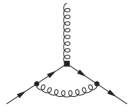
(b) vertex corrections

Figure 1: Feynman diagrams for the calculation of the anomalous dimension for the charged electroweak case.

We focus on QCD effects only and consider the diagrams shown in Figs. 1(a) and 1(b). The left- and right-handed current do not have an anomalous dimension, and hence

$$L^{q}_{1}(m_{t})=L^{q}_{1}(\Lambda),\quad R^{q}_{1}(m_{t})=R^{q}_{1}(\Lambda)\ .$$ (35)

The helicity-changing contributions have an anomalous dimension which has to be equal for both helicity combinations. To leading order one finds

$$\gamma^{T}(\alpha_{s})=\frac{2\alpha_{s}}{3\pi},$$ (36)

which yields for the running from $\Lambda$ to $\mu\sim m_{t}$ for the two remaining couplings

$$\begin{split}L^{q}_{2}(m_{t})&=L^{q}_{2}(\Lambda)\left(\frac{\alpha_{s}(\Lambda)}{\alpha_{s}(m_{t})}\right)^{\frac{4}{3\beta_{0}}},\\ R^{q}_{2}(m_{t})&=R^{q}_{2}(\Lambda)\left(\frac{\alpha_{s}(\Lambda)}{\alpha_{s}(m_{t})}\right)^{\frac{4}{3\beta_{0}}},\end{split}$$ (37)

with

$$\beta_{0}=\frac{11n_{c}-2n_{f}}{3},$$ (38)

where $n_{c}$ and $n_{f}$ are the numbers of colours and quark flavours, respectively.

From the effective operators we may calculate the amplitudes for top decays, taking into account a possible NP effect. To this end, we use Eq. (32) and compute the decay rates for the decay of an unpolarized top-quark into a down-type quark $q$ and an on-shell $W$ boson. The analysis of the $W$-decay products allows us to reconstruct its polarization, which is either longitudinal, left-, or right-handed. The corresponding rates read Kane:1991bg ; AguilarSaavedra:2006fy

$$\Gamma(t\to qW_{0}) = \frac{g_{2}^{2}|\vec{q}|}{32\pi}\left\{\frac{m_{t}^{2}}{M_{W}^{2}}\left[|L^{q}_{1}|^{2}+|R^{q}_{1}|^{2}\right]\left(1-x_{W}^{2}-2x_{q}^{2}-x_{W}^{2}x_{q}^{2}+x_{q}^{4}\right)-4x_{q}{\rm Re}\left\{L^{q}_{1}R^{q\ast}_{1}\right\}\right.$$ (39)

$$\qquad\qquad\,\,+\left[|L^{q}_{2}|^{2}+|R^{q}_{2}|^{2}\right]\left(1-x_{W}^{2}+x_{q}^{2}\right)-4x_{q}{\rm Re}\left\{L^{q}_{2}R^{q\ast}_{2}\right\}$$

$$\qquad-2\frac{m_{t}}{M_{W}}{\rm Re}\left(L^{q}_{1}R^{q\ast}_{2}+L^{q}_{2}R^{q\ast}_{1}\right)\left(1-x_{W}^{2}-x_{q}^{2}\right)$$

$$\qquad\left.+2\frac{m_{t}}{M_{W}}x_{q}{\rm Re}\left\{L^{q}_{1}L^{q\ast}_{2}+R^{q}_{2}R^{q\ast}_{1}\right\}\left(1+x_{W}^{2}-x_{q}^{2}\right)\right\}\allowdisplaybreaks$$

$$\Gamma(t\to qW_{L/R}) = \frac{g_{2}^{2}|\vec{q}|}{32\pi}\left\{\left[|L^{q}_{1}|^{2}+|R^{q}_{1}|^{2}\right]\left(1-x_{W}^{2}+x_{q}^{2}\right)-4x_{q}{\rm Re}\left\{L^{q}_{1}R^{q\ast}_{1}\right\}\right.$$ (40)

$$\qquad+\frac{m_{t}^{2}}{M_{W}^{2}}\left[|L^{q}_{2}|^{2}+|R^{q}_{2}|^{2}\right]\left(1-x_{W}^{2}-2x_{q}^{2}-x_{W}^{2}x_{q}^{2}+x_{q}^{4}\right)-4x_{q}{\rm Re}\left\{L^{q}_{2}R^{q\ast}_{2}\right\}$$

$$\qquad-2\frac{m_{t}}{M_{W}}{\rm Re}\left\{L^{q}_{1}R^{q\ast}_{2}+L^{q}_{2}R^{q\ast}_{1}\right\}\left(1-x_{W}^{2}-x_{q}^{2}\right)$$

$$\qquad\left.+2\frac{m_{t}}{M_{W}}x_{q}{\rm Re}\left\{L^{q}_{1}L^{q\ast}_{2}+R^{q}_{2}R^{q\ast}_{1}\right\}\left(1+x_{W}^{2}-x_{q}^{2}\right)\right\}\allowdisplaybreaks$$

$$\pm \frac{g_{2}^{2}m_{t}}{64\pi}\frac{m_{t}^{2}}{M_{W}^{2}}\left\{-x_{W}^{2}\left[|L^{q}_{1}|^{2}-|R^{q}_{1}|^{2}\right]+\left[|L^{q}_{2}|^{2}+|R^{q}_{2}|^{2}\right]\left(1-x_{q}^{2}\right)\vphantom{\frac{1}{1}}\right.\allowdisplaybreaks$$

$$\left.\vphantom{\frac{1}{1}}\qquad\quad\qquad+2x_{W}{\rm Re}\left\{L^{q}_{1}R^{q\ast}_{2}-L^{q}_{2}R^{q\ast}_{1}\right\}+2x_{W}x_{q}{\rm Re}\left\{L^{q}_{1}L^{q\ast}_{2}-R^{q}_{2}R^{q\ast}_{1})\right\}\right\}$$

$$\qquad\quad\qquad\quad\qquad\times\left(1-2x_{W}^{2}-2x_{q}^{2}+x_{W}^{4}-2x_{W}^{2}x_{q}^{2}+x_{q}^{4}\right)$$

where the upper sign holds for left-handed and the lower sign for right-handed $W$ bosons. Furthermore, $x_{q}\equiv m_{q}/m_{t}$, $x_{W}\equiv M_{W}/m_{t}$,

$$|\vec{p}|=\frac{m_{t}}{2}\sqrt{\lambda(1,x_{q}^{2},x_{W}^{2})},$$ (41)

and the Källén function $\lambda(a,b,c)\equiv(a-b-c)^{2}-4bc$.

The total rate $\Gamma(t\to qW)$ is given by the sum

$$\Gamma(t\to qW) = \Gamma(t\to qW_{0})+\Gamma(t\to qW_{L})$$ (42)

$$+\Gamma(t\to qW_{R}),$$

and the corresponding observables are the helicity fractions $F_{0}=\Gamma(t\to qW_{0})/\Gamma(t\to qW)$, $F_{L}=\Gamma(t\to qW_{L})/\Gamma(t\to qW)$ and $F_{R}=\Gamma(t\to qW_{R})/\Gamma(t\to qW)$. Using the condition $F_{0}+F_{R}+F_{L}\equiv 1$ we get for the normalised differential decay rate Kane:1991bg ; AguilarSaavedra:2006fy ,

$$\frac{1}{\Gamma}\frac{d\Gamma}{d\cos\theta^{\ast}} = \frac{3}{8}\left(1-\cos\theta^{\ast}\right)^{2}F_{L}+\frac{3}{8}\left(1+\cos\theta^{\ast}\right)^{2}F_{R}$$ (43)

$$+\frac{3}{4}\sin^{2}\theta^{\ast}F_{0},$$

with the helicity angle $\theta^{\ast}$, defined as the angle between the charged lepton three-momentum in the $W$-boson rest frame and the $W$-boson momentum in the top-quark rest frame.

The latest experimental measurements from ATLAS ATLAS-CONF-2011-122 and CMS CMS-PAS-TOP-11-020 are shown in Table 1.

Table 1: Helicity fractions @95% C.L. from ATLAS and CMS for $t\to bW$ decay (see text for references). The errors are statistical and systematic, respectively.

Fraction	ATLAS	CMS
$F_{0}$	$0.57\pm 0.07\pm 0.09$	$0.567\pm 0.074\pm 0.047$
$F_{L}$	$0.35\pm 0.04\pm 0.04$	$0.393\pm 0.045\pm 0.029$
$F_{R}$	$0.09\pm 0.04\pm 0.08$	$0.040\pm 0.035\pm 0.044$

For a quantiative analysis we adopt the scheme described above. This means in particular, that we take the relations (34) as equalities, and that we analyse the data in terms of the single quantity

$$\delta L^{q}_{1}=\alpha\frac{v^{2}}{\Lambda^{2}},$$ (44)

where $\alpha$ would be unity in a tree-induced scenario, while $\alpha=1/(16\pi^{2})$ in a loop-induced scenario. In Fig. 2 we plot the helicity fraction $F_{L}$ and $F_{R}$ for $t\to bW$ as as function of $\delta L^{3}_{1}$. The standard model value corresponds to $\delta L^{q}_{1}\equiv 0$ up to very small radiative corrections. The colored bands indicate the data shown in Table 1. From this we infer that the SM value is well compatible with the current data. However, given the current uncertainties, there is still some room for a nonvanishing $\delta L^{q}_{1}$. It is interesting to note that for both helicity fractions a region around $\delta L^{q}_{1}\sim 0.4$ is still allowed, while the other region constrains $|\delta L^{q}_{1}|\leq 0.1$.

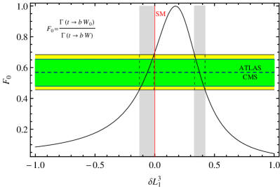
Figure 2: Helicity fractions $F_{L}$ (top) and $F_{0}$ (bottom) for the decay $t\to bW$ as a function of a possible MFV new physics contribution with the coupling $\delta L^{q}_{1}$. The horizontal bands indicate the current data from the LHC experiments, while the vertical bands indicate the currently allowed range for $\delta L^{q}_{1}$.

The parameter $\delta L^{q}_{1}$ still contains the dependence on $\Lambda$, the scale of new physics. Assuming a value of $\Lambda\sim 1$ TeV we end up with $v^{2}/\Lambda^{2}\sim 0.1$. This implies for NP scales around 1 TeV that the couplings in Eq. (33) can still be as large as unity, implying that the current sensitivity cannot rule out MFV new physics effects at tree level. In turn, in the loop-induced scenario there is still plenty of room for NP effects.

IV.2 Neutral Currents

The study of FCNCs such as $t\to qV$, $q\in\{u,c\}$, $V\in\{Z,\gamma,g\}$ is important in the context of NP analyses, since the contribution of the SM is highly Glashow-Iliopoulos-Maiani (GIM) suppressed Glashow:1970gm . A measurement of such a process at the current level of sensitivity would clearly indicate new physics, in particular also implying non-MFV effects; the SM branching ratios ($\mathscr{B}$) are in the region $\mathscr{B}(t\to qZ)\sim\mathcal{O}(10^{-13})$, $\mathscr{B}(t\to q\gamma)\sim\mathcal{O}(10^{-13})$ and $\mathscr{B}(t\to qg)\sim\mathcal{O}(10^{-11})$ Grzadkowski:1990sm .

Table 2: List of operators for $t\to qV$, $q\in\{u,c\}$, $V\in\{Z,\gamma,g\}$ transitions.

Decay	Operator
$t\to qZ$	$\mathcal{O}^{ij(3)}_{\rm LL}$, $\mathcal{O}^{ij(4)}_{\rm LL}$, $\mathcal{O}^{ij(5)}_{\rm LL}$, $\mathcal{O}^{ij(6)}_{\rm LL}$
	$\mathcal{O}^{ij(2)}_{\rm RR}$, $\mathcal{O}^{ij(4)}_{\rm LR}$, $\mathcal{O}^{ij(5)}_{\rm LR}$
$t\to q\gamma$	$\mathcal{O}^{ij(4)}_{\rm LR}$, $\mathcal{O}^{ij(5)}_{\rm LR}$
$t\to qg$	$P^{ij(5)}_{\rm LR}$

The operators contributing to the FCNC interactions are listed in Table 2. The experimental signatures of the various channels are quite different, so we study the different processes separately in the following.

IV.2.1 $t\to qZ$

The effective Lagrangian for the neutral currents involving the $Z_{0}$ can be written as

$$\mathscr{L}_{\rm eff} = \frac{g_{2}}{\cos\theta_{W}}Z_{\mu}$$ (45)

$$\times\biggl{\{}\bar{q}\gamma^{\mu}\left(L^{\prime q}_{1}P_{L}+R^{\prime q}_{1}P_{R}\right)t$$

$$-\frac{(i\partial_{\nu})}{M_{Z}}\left[\bar{q}i\sigma^{\mu\nu}\left(L^{\prime q}_{2}P_{L}+R^{\prime q}_{2}P_{R}\right)t\right]\biggr{\}},$$

with the couplings

$$L^{\prime q}_{1} = V_{qb}V^{\ast}_{tb}\left[\eta^{(3)}_{\rm LL}\frac{m_{b}^{2}}{\Lambda^{2}}+\eta^{(4)}_{\rm LL}\frac{m_{b}^{2}}{\Lambda^{2}}\tan^{2}\beta\right.\left.-\frac{\eta^{(5)}_{\rm LL}}{2}\frac{m_{b}^{2}}{\Lambda^{2}}-\frac{\eta^{(6)}_{\rm LL}}{2}\frac{m_{b}^{2}}{\Lambda^{2}}\tan^{2}\beta\right],\allowdisplaybreaks$$ (46)

$$R^{\prime q}_{1} = V_{qb}V^{\ast}_{tb}\alpha^{(2)}_{\rm RR}\frac{m_{b}^{2}}{\Lambda^{2}}\frac{m_{q}m_{t}}{v^{2}}\frac{1}{\sin^{2}\beta},\allowdisplaybreaks$$ (47)

$$L^{\prime q}_{2} = 2V_{qb}V^{\ast}_{tb}\frac{m_{q}}{v}\frac{1}{\sin^{2}\beta}\biggl{(}\cos\theta_{W}\alpha^{(4)\ast}_{\rm LR}\frac{m_{b}^{2}}{\Lambda^{2}}-\sin\theta_{W}\alpha^{(5)\ast}_{\rm LR}\frac{m_{b}^{2}}{\Lambda^{2}}\biggr{)},\allowdisplaybreaks$$ (48)

$$R^{\prime q}_{2} = 2V_{qb}V^{\ast}_{tb}\frac{m_{t}}{v}\frac{1}{\sin^{2}\beta}\biggl{(}\cos\theta_{W}\alpha^{(4)}_{\rm LR}\frac{m_{b}^{2}}{\Lambda^{2}}-\sin\theta_{W}\alpha^{(5)}_{\rm LR}\frac{m_{b}^{2}}{\Lambda^{2}}\biggr{)},$$ (49)

where $\theta_{W}$ is the Weinberg angle.

As an order-of-magnitude estimate, it is worthwhile to note that MFV leads to a significant GIM-like suppression of this coupling by a factor of $m_{b}^{2}/\Lambda^{2}$, which is much smaller than the “natural” value of the coupling $v^{2}/\Lambda^{2}$. Furthermore, also for the relative sizes of the couplings for the various helicity combinations, we get an MFV prediction $\tan\beta\sim 1$ or larger

$$\begin{split}R^{\prime q}_{1}&\sim L^{\prime q}_{1}\frac{m_{q}m_{t}}{v^{2}}\frac{1}{\tan^{2}\beta},\\ L^{\prime q}_{2}&\sim L^{\prime q}_{1}\frac{m_{q}}{v}\frac{1}{\tan^{2}\beta},\\ R^{\prime q}_{2}&\sim L^{\prime q}_{1}\frac{m_{t}}{v}\frac{1}{\tan^{2}\beta},\end{split}$$ (50)

Finally we note that there is also a loop-induced contribution from the SM which has been calculated in Ref. AguilarSaavedra:2002ns . However, the relevant vertex cannot be expressed as a local operator, and hence the expressions are quite cumbersome. On the other hand, since the SM is by construction MFV, the same suppression factors as for the new physics contribution will appear, and since the SM rates are tiny compared to the current experimental limit we take for the SM contribution the simple estimates

$$L^{\prime q}_{1{\rm SM}} = V_{qb}V^{\ast}_{tb}\frac{1}{16\pi^{2}}\frac{m_{b}^{2}}{v^{2}},$$ (51)

$$R^{\prime q}_{1{\rm SM}} = V_{qb}V^{\ast}_{tb}\frac{1}{16\pi^{2}}\frac{m_{b}^{2}}{v^{2}}\frac{m_{q}m_{t}}{v^{2}},$$

$$L^{\prime q}_{2{\rm SM}} = R^{\prime q}_{2{\rm SM}}=V_{qb}V^{\ast}_{tb}\frac{1}{16\pi^{2}}\frac{m_{b}^{2}}{v^{2}}\frac{m_{t}}{v},$$

which is numerically very close to the real calculation, i.e. it yields a branching fraction of the order

$$\mathscr{B}_{\rm SM}(t\to cZ)\sim\left|\frac{1}{16\pi^{2}}V_{cb}\frac{m_{b}^{2}}{v^{2}}\right|^{2}\sim 6\times 10^{-15}\ .$$ (52)

In order to perform a numerical analysis we proceed similarly to the case of charged currents. We take the approximate relations (50) as exact equations and express everything in terms of the new physics coupling $L^{\prime q}_{1}$. Including the standard model estimate on the basis of the naive estimate (51) we show in Fig. 3 the branching fraction for $t\to qZ$, $q\in\{u,c\}$.

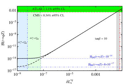
Figure 3: The branching fraction for $t\to Zq$ as a function of the coupling $L^{\prime q}_{1}$ and $\tan\beta=10$. The horizontal lines indicate the expectation within the SM and the current limits imposed by ATLAS CortesGonzalez:2012ym ; ATLAS-CONF-2011-154 and CMS CMS-PAS-TOP-11-028 .

We note that the natural size of $L^{\prime q}_{1}$ is in MFV given by $V_{qb}V_{tb}^{\ast}m_{b}^{2}/\Lambda^{2}$, assuming tree-level FCNC effects. This is for $\Lambda\sim 1$ TeV about $10^{-6}$, which is one order of magnitude above the SM value. Loop-induced new physics effects would show up in MFV for $\Lambda\sim 1$ TeV only at a level of $L^{\prime q}_{1}\sim 10^{-9}$, which is far below the SM value. In turn, the current experimental limit implies $L^{\prime q}_{1}\leq 0.01$, which is far above the prediction of any MFV scenario.

IV.2.2 $t\to q\gamma$ and $t\to qg$

The possible couplings for photonic transitions are more restricted due to electromagnetic gauge invariance. Extracting the relevant terms form the dimension-6 operators we find for the effective Lagrangian

$$\mathscr{L}_{\rm eff}=-e\mathcal{A}_{\mu}\frac{(i\partial_{\nu})}{m_{t}}\left[\bar{q}i\sigma^{\mu\nu}\left(L^{(2)}_{q}P_{L}+R^{(2)}_{q}P_{R}\right)t\right],$$ (53)

where $e$ and $\mathcal{A}_{\mu}$ are the electron charge and the electromagnetic field, respectively.

For the $\gamma tq$ vertex we get only two independent anomalous coupling constants,

$$\begin{split}L^{(2)}_{q}&=\frac{4V_{qb}V^{\ast}_{tb}}{e}\left(\sin\theta_{W}\mathcal{C}^{32(4)\ast}_{\rm LR}+\cos\theta_{W}\mathcal{C}^{32(5)\ast}_{\rm LR}\right)\frac{m_{b}^{2}}{\Lambda^{2}}\frac{m_{q}m_{t}}{v_{1}^{2}},\\ R^{(2)}_{q}&=\frac{4V_{qb}V^{\ast}_{tb}}{e}\left(\sin\theta_{W}\mathcal{C}^{23(4)}_{\rm LR}+\cos\theta_{W}\mathcal{C}^{23(5)}_{\rm LR}\right)\frac{m_{b}^{2}}{\Lambda^{2}}\frac{m_{t}^{2}}{v_{1}^{2}}.\end{split}$$ (54)

Clearly, in a MFV scenario, the right-handed top quark yields the dominant contribution,

$$L^{(2)}_{q}\sim\frac{m_{q}}{m_{t}}R^{(2)}_{q}\ .$$ (55)

Taking this as an equation, we can express the rate and the branching fractions in terms of the single coupling $R^{(2)}_{q}$.

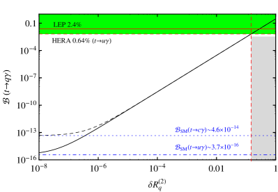
Figure 4: The branching fraction for $t\to q\gamma$ as a function of the coupling $L^{\prime q}_{1}$. The horizontal lines indicate the expectation within the SM and the current limits imposed by LEP Heister:2002xv ; Abdallah:2003wf ; Abbiendi:2001wk ; Achard:2002vv ; LEP-Exotica:WG-2001-01 and HERA $(t\to u\gamma)$ Aaron:2009vv , and also from Tevatron: 3.2% Abe:1997fz which is not shown.

The standard model value for this process is very small. This can be inferred already from a simple order-of-magnitude estimate by just collecting the factors for the loop suppression and the CKM and mass factors. One obtains

$$\mathscr{B}_{\rm SM}(t\to q\gamma) \sim \left|\frac{\alpha}{\pi}V_{tb}V_{qb}^{\ast}\frac{m_{b}^{2}}{M_{W}^{2}}\frac{m_{t}^{2}}{v^{2}}\right|^{2}$$ (56)

$$\sim \begin{cases}4\times 10^{-14}&{\rm for}\quad t\to c\gamma\\ 4\times 10^{-16}&{\rm for}\quad t\to u\gamma\end{cases}$$

which is numerically close to the values obtained from the full calculation.

As in the case of $t\to Zq$, the MFV expectation is very small. Assuming a tree-like scenario, $R^{(2)}_{q}$ is of the order $V_{qb}V^{\ast}_{tb}m_{b}^{2}/\Lambda^{2}$. For a new physics scale $\Lambda\sim 1$ TeV we end up with a typical expectation $R^{(2)}_{c}\sim 10^{-7}$ and $R^{(2)}_{u}\sim 10^{-8}$ for the loop-induced scenario; this is even smaller by a factor of $1/(16\pi^{2})$. Thus, if nature is minimally flavour violating, but otherwise the couplings have natural sizes, the current limits are several orders of magnitude above the expectations.

The case $t\to gq$ is very similar to $t\to q\gamma$; the only difference is the larger strong coupling and larger QCD renormalization effects. The one-loop QCD renormalization is given in Appendix A; although the effects can be sizable, they are still far away from being relevant in the current experimental situation.

Due to QCD gauge invariance the effective interaction has a similar form as the photonic operator,

$$\mathscr{L}_{\rm eff} = -g_{s}G_{\mu}^{a}\frac{1}{m_{t}}$$ (57)

$$\times(-i\partial_{\nu})\left[\bar{q}T^{a}i\sigma^{\mu\nu}\left(\tilde{L}^{(2)}_{q}P_{L}+\tilde{R}^{(2)}_{q}P_{R}\right)t\right],$$

with

$$\tilde{L}^{(2)}_{q} =V_{qb}V^{\ast}_{tb}\frac{4}{g_{s}}K^{32(5)\ast}_{\rm LR}\frac{m_{b}^{2}}{\Lambda^{2}}\frac{m_{q}m_{t}}{v_{1}^{2}},$$ (58)

$$\tilde{R}^{(2)}_{q} =V_{qb}V^{\ast}_{tb}\frac{4}{g_{s}}K^{23(5)}_{\rm LR}\frac{m_{b}^{2}}{\Lambda^{2}}\frac{m_{t}^{2}}{v_{1}^{2}},$$ (59)

where $G^{a}_{\mu}$ is the field strength-tensor of the gluon fields and $T^{a}$ are the Gell-Mann matrices.

For $K^{32(5)}_{\rm LR},K^{23(5)}_{\rm LR}\sim 1$ we get the same order-of-magnitude relation for the couplings as for the photonic case

$$\tilde{L}^{(2)}_{q}\sim\frac{m_{q}}{m_{t}}\tilde{R}^{(2)}_{q},$$ (60)

and we shall again use this as an equality to perform an MFV analysis in terms of the single variable. Figure 5 shows the current status.

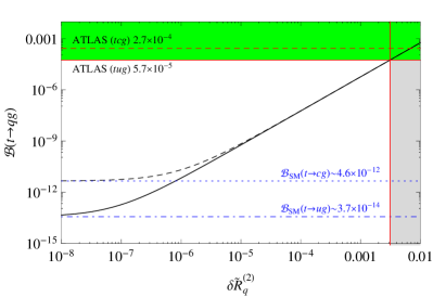
Figure 5: The branching fraction for $t\to qg$ as a function of the coupling $\tilde{R}^{(2)}_{q}$. The horizontal lines indicate the expectation within the SM and the current limits imposed by ATLAS Collaboration:2012gd .

The estimate in the standard model is the same as for $t\to q\gamma$ with the electromagnetic coupling replaced by the strong one,

$$\mathscr{B}_{\rm SM}(t\to qg) \sim \left|\frac{\alpha_{s}}{\pi}V_{tb}V_{qb}^{\ast}\frac{m_{b}^{2}}{M_{W}^{2}}\frac{m_{t}^{2}}{v^{2}}\right|^{2}$$ (61)

$$\sim \begin{cases}6\times 10^{-12}&{\rm for}\quad t\to cg\\ 4\times 10^{-14}&{\rm for}\quad t\to ug\end{cases}$$

which again is close to the result of the full calculation. Concerning the expectations of the MFV scenario, one arrives at the same conclusions as for $t\to q\gamma$: the MFV expectations are still several orders of magnitude away from the experimental sensitivity.

V Comparison to other constraints

Aside from direct searches, indirect constraints may also be obtained from both electroweak as well as from $B$ and $K$ decays.

The assumption of MFV also links the flavour physics of the top quark with that of the bottom and the strange quark. Overall, the constraints from $B$ and $K$ physics which are discussed at length in Refs. D'Ambrosio:2002ex ; Hurth:2008jc , are much more restrictive than the ones obtained from the current data on the top quark. In turn, any effect that could be seen in top decays at the current level of precision would indicate a deviation from MFV.

A certain loophole in the MFV argument emerges due to the large top-quark mass, implying an order unity Yukawa coupling for the top. This may be closed by employing a nonlinear realization of MFV Feldmann:2008ja ; however, as discussed in Ref. Kagan:2009bn , some effects may become visible in the top sector for large values of $\tan\beta$.

Another way of testing anomalous $t\to bW$ couplings is in loop-induced $B$ decays. It has been shown in Ref. Grzadkowski:2008mf that in particular the decay $B\to X_{s}\gamma$ is quite sensitive to an anomalous $t\to bW$ coupling resulting in a limit. The combined analyses performed in Refs. Drobnak:2011aa ; Drobnak:2011wj , including also other FCNC processes of $B$ mesons, arrives at bounds for anomalous $t\to bW$ couplings which are again stronger than what can be obtained from the current direct measurements at the LHC.

Also the precision data from the electroweak sector constrain possible nonstandard top couplings. Such an analysis, using the precision data on the oblique parameters of the electroweak sector, has been performed in Ref. Zhang:2012cd . The constraints obtained in this way are comparable to the ones obtained from flavour decays and thus are again much stronger than the bounds from the currently available direct measurements.

VI Conclusions

We have discussed anomalous, flavour-changing top decays in a model-independent way by employing an effective field theory approach. The new element in our analysis is the implementation of minimal flavour violation by setting up a simple scheme with few parameters, which obeys the MFV hierarchical structure. We have calculated the decay rates for the charged current $t\to qW$, $q\in\{d,s,b\}$, as well as for the FCNC couplings $tqV$, $q\in\{u,c\}$, $V\in\{Z,\gamma,g\}$, in terms of the effective couplings for different helicities under the assumption that the top quark is produced in a high-energy collision as a quasi-free particle. Comparing such a scenario with the present data shows that there is still plenty of room for NP effects in the anomalous, flavour-changing top couplings, in particular for the flavour-changing neutral current decays.

Appendix A QCD Renormalization

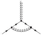
(a)

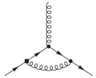
(b)

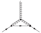
(c)

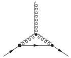
(d)

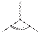
(e)

(f)

Figure 6: Feynman diagrams for the calculation of the anomalous dimension for the strong decays. Diagrams (e) and (f) include a mixing of strong and electroweak interactions.

The calculation of the anomalous dimension for the $t\to qV$ transitions proceeds along the same lines as we discussed in Sec. IV.1 for the charged current. However, for the QCD-like structure of the generalised $gtq$ vertex, Eq. (57), additional diagrams have to be taken into account. All Feynman diagrams shown in Fig. 6 – where Figs. 6(e) and 6(f) represent the mixing of strong and electroweak operators – have to be calculated. We define

$$\vec{\mathcal{C}} = \begin{pmatrix}\tilde{L}^{(2)}_{q}\\ \tilde{R}^{(2)}_{q}\\ L^{(2)}_{q}\\ R^{(2)}_{q}\\ L^{\prime q}_{2}\\ R^{\prime q}_{2}\end{pmatrix},\allowdisplaybreaks$$ (62)

$$\vec{\mathcal{O}} = \left(-i\partial_{\nu}\right)\left(\bar{q}\sigma^{\mu\nu}\begin{pmatrix}\frac{1}{m_{t}}T_{a}P_{L}G^{a}_{\mu}\\ \frac{1}{m_{t}}T_{a}P_{R}G^{a}_{\mu}\\ \frac{1}{m_{t}}P_{L}\mathcal{A}_{\mu}\\ \frac{1}{m_{t}}P_{R}\mathcal{A}_{\mu}\\ \frac{1}{M_{Z}}P_{L}Z_{\mu}\\ \frac{1}{M_{z}}P_{R}Z_{\mu}\\ \end{pmatrix}t\right),$$ (63)

and for the $6\times 6$ anomalous-dimension matrix for the Wilson coefficients, using Feynman gauge, we get

$$\gamma^{T}(\mu)=\frac{2\alpha_{s}(\mu)}{3\pi}\begin{pmatrix}-\frac{215}{32}&0&0&0&0&0\\ 0&-\frac{215}{32}&0&0&0&0\\ 3&0&1&0&0&0\\ 0&3&0&1&0&0\\ \cos(2\theta_{W})-\frac{1}{4}&0&0&0&1&0\\ 0&\cos(2\theta_{W})-\frac{1}{4}&0&0&0&1\end{pmatrix}\ .$$ (64)

This matrix describes the mixing of QCD-like operators and neutral weak electroweak operators and determines the running of the Wilson coefficients.

The solution of the renormalization-group equation,

$$\frac{d\vec{\mathcal{C}}}{d\ln\mu}=\gamma^{T}(\mu)\cdot\vec{\mathcal{C}},$$ (65)

is straightforward, and we find

$$\tilde{I}^{(2)}_{q}(\mu) = \tilde{I}^{(2)}_{q}(\Lambda)\left(\frac{\alpha_{s}(\Lambda)}{\alpha_{s}(\mu)}\right)^{-\frac{215}{24\beta_{0}}},$$ (66)

$$I^{(2)}_{q}(\mu) = \left[3\tilde{I}^{(2)}_{q}(\Lambda)+I^{(2)}_{q}(\Lambda)\right]\left(\frac{\alpha_{s}(\Lambda)}{\alpha_{s}(\mu)}\right)^{\frac{4}{3\beta_{0}}}-3\tilde{I}^{(2)}_{q}(\Lambda)\left(\frac{\alpha_{s}(\Lambda)}{\alpha_{s}(\mu)}\right)^{-\frac{215}{24\beta_{0}}},\allowdisplaybreaks$$ (67)

$$I^{\prime q}_{2}(\mu) = \left[\left(\cos(2\theta_{W})-\frac{1}{4}\right)\tilde{I}^{(2)}_{q}(\Lambda)+I^{\prime q}_{2}(\Lambda)\right]\left(\frac{\alpha_{s}(\Lambda)}{\alpha_{s}(\mu)}\right)^{\frac{4}{3\beta_{0}}}$$ (68)

$$-\left(\cos(2\theta_{W})-\frac{1}{4}\right)\tilde{I}^{(2)}_{q}(\Lambda)\left(\frac{\alpha_{s}(\Lambda)}{\alpha_{s}(\mu)}\right)^{-\frac{215}{24\beta_{0}}},$$

with $I\in\{L,R\}$. The scale dependencies of $L^{\prime q}_{1}$ and $R^{\prime q}_{1}$ are given by

$$L^{\prime q}_{1}(\mu)=L^{\prime q}_{1}(\Lambda),\ R^{\prime q}_{1}(\mu)=R^{\prime q}_{1}(\Lambda)\ .$$ (69)

With these relations it is not difficult to check the logarithmic terms of the one-loop calculation including the logarithmic corrections to every order in $\alpha_{s}\ln\Lambda/\mu$, $\mu\sim m_{t}$.

References

- (1) Tevatron Electroweak Working Group, for the CDF and DØ Collaborations(2011), arXiv:1107.5255 [hep-ex]
- (2) e. Evans, Lyndon and e. Bryant, Philip, JINST 3, S08001 (2008)
- (3) M. Beneke et al.(2000), arXiv:hep-ph/0003033 [hep-ph]
- (4) W. Bernreuther, J.Phys.G G35, 083001 (2008), arXiv:0805.1333 [hep-ph]
- (5) S. Willenbrock, EPJ Web Conf. 28, 05005 (2012), arXiv:1205.4676 [hep-ph]
- (6) C. Zhang, N. Greiner, and S. Willenbrock, Phys.Rev. D86, 014024 (2012), arXiv:1201.6670 [hep-ph]
- (7) C. Zhang and S. Willenbrock, Phys.Rev. D83, 034006 (2011), arXiv:1008.3869 [hep-ph]
- (8) J. Aguilar-Saavedra, Acta Phys.Polon. B35, 2695 (2004), arXiv:hep-ph/0409342 [hep-ph]
- (9) G. Aad et al. (ATLAS Collaboration), Phys.Lett. B716, 1 (2012), arXiv:1207.7214 [hep-ex]
- (10) S. Chatrchyan et al. (CMS Collaboration), Phys.Lett. B716, 30 (2012), arXiv:1207.7235 [hep-ex]
- (11) J. F. Gunion et al., Front.Phys. 80, 1 (2000)
- (12) J. F. Donoghue and L. F. Li, Phys.Rev. D19, 945 (1979)
- (13) L. J. Hall and M. B. Wise, Nucl.Phys. B187, 397 (1981)
- (14) C. Burges and H. J. Schnitzer, Nucl.Phys. B228, 464 (1983)
- (15) C. N. Leung et al., Z.Phys. C31, 433 (1986)
- (16) W. Buchmüller and D. Wyler, Nucl.Phys. B268, 621 (1986)
- (17) T. Hansmann and T. Mannel, Phys.Rev. D68, 095002 (2003), arXiv:hep-ph/0306043 [hep-ph]
- (18) F. Bach and T. Ohl, Phys.Rev. D86, 114026 (2012), arXiv:1209.4564 [hep-ph]
- (19) S. L. Glashow and S. Weinberg, Phys.Rev. D15, 1958 (1977)
- (20) A. Ali and D. London, Eur.Phys.J. C9, 687 (1999), arXiv:hep-ph/9903535 [hep-ph]
- (21) A. Buras, P. Gambino, M. Gorbahn, S. Jager, and L. Silvestrini, Phys.Lett. B500, 161 (2001), arXiv:hep-ph/0007085 [hep-ph]
- (22) G. D’Ambrosio et al., Nucl.Phys. B645, 155 (2002), arXiv:hep-ph/0207036 [hep-ph]
- (23) T. Feldmann and T. Mannel, Phys.Rev.Lett. 100, 171601 (2008), arXiv:0801.1802 [hep-ph]
- (24) G. L. Kane, G. Ladinsky, and C. Yuan, Phys.Rev. D45, 124 (1992)
- (25) J. Aguilar-Saavedra, J. Carvalho, N. F. Castro, F. Veloso, and A. Onofre, Eur.Phys.J. C50, 519 (2007), arXiv:hep-ph/0605190 [hep-ph]
- (26) [The ATLAS Collaboration], Measurement of the W boson polarisation in top quark decays in 0.70 fb-1 of pp collisions at sqrt(s)=7 TeV with the ATLAS detector, Tech. Rep. ATLAS-CONF-2011-122 (2011)
- (27) [The CMS Collaboration], W helicity in top pair events, Tech. Rep. CMS PAS TOP-11-020 (2012)
- (28) S. Glashow, J. Iliopoulos, and L. Maiani, Phys.Rev. D2, 1285 (1970)
- (29) B. Grzadkowski, J. Gunion, and P. Krawczyk, Phys.Lett. B268, 106 (1991)
- (30) J. Aguilar-Saavedra and B. Nobre, Phys.Lett. B553, 251 (2003), arXiv:hep-ph/0210360 [hep-ph]
- (31) A. Cortes-Gonzalez(2012), arXiv:1201.4308 [hep-ex]
- (32) [The ATLAS Collaboration], A search for Flavour Changing Neutral Currents in Top Quark Decays at TeV in 0.70 fb-1 of collision data collected with the ATLAS Detector, Tech. Rep. ATLAS-CONF-2011-154 (2011)
- (33) [The CMS Collaboration], Search for , Tech. Rep. CMS PAS TOP-11-028 (2012)
- (34) A. Heister et al. (ALEPH Collaboration), Phys.Lett. B543, 173 (2002), arXiv:hep-ex/0206070 [hep-ex]
- (35) J. Abdallah et al. (DELPHI Collaboration), Phys.Lett. B590, 21 (2004), arXiv:hep-ex/0404014 [hep-ex]
- (36) G. Abbiendi et al. (OPAL Collaboration), Phys.Lett. B521, 181 (2001), arXiv:hep-ex/0110009 [hep-ex]
- (37) P. Achard et al. (L3 Collaboration), Phys.Lett. B549, 290 (2002), arXiv:hep-ex/0210041 [hep-ex]
- (38) [The LEP Exotica WG], Search for single top production via flavour changing neutral currents: preliminary combined results of the LEP experiments., Tech. Rep. LEP-Exotica-WG-2001-01. (CERN, Geneva, 2001)
- (39) F. Aaron et al. (H1 Collaboration), Phys.Lett. B678, 450 (2009), arXiv:0904.3876 [hep-ex]
- (40) F. Abe et al. (CDF Collaboration), Phys.Rev.Lett. 80, 2525 (1998)
- (41) G. Aad et al. (ATLAS Collaboration)(2012), arXiv:1203.0529 [hep-ex]
- (42) T. Hurth, G. Isidori, J. F. Kamenik, and F. Mescia, Nucl.Phys. B808, 326 (2009), arXiv:0807.5039 [hep-ph]
- (43) A. L. Kagan, G. Perez, T. Volansky, and J. Zupan, Phys.Rev. D80, 076002 (2009), arXiv:0903.1794 [hep-ph]
- (44) B. Grzadkowski and M. Misiak, Phys.Rev. D78, 077501 (2008), arXiv:0802.1413 [hep-ph]
- (45) J. Drobnak, S. Fajfer, and J. F. Kamenik, Nucl.Phys. B855, 82 (2012), arXiv:1109.2357 [hep-ph]
- (46) J. Drobnak, S. Fajfer, and J. F. Kamenik, Phys.Lett. B701, 234 (2011), arXiv:1102.4347 [hep-ph]