Dynamical entanglement in coupled optical cavities

Abstract

We study the evolution of a photonic state in a coupled pair of anharmonic cavities and compare it with the corresponding system of two coupled harmonic cavities. The photons in the anharmonic cavities interact with a two-level atom and are described within the Jaynes-Cummings model. Starting from an eigenstate of the Jaynes-Cummings model with $N$ photons, the evolution of this state in the presence of photon tunneling between the cavities is studied. We evaluate the spectral density, the dynamics of the return as well as the transition amplitudes and the probability for the dynamical creation of a N00N state.

I Introduction

The dynamics of isolated many-body quantum systems has been a subject of intense research in atomic physics during recent years, in experiment atoms as well as in theory yukalov09 . This interest has two major aspects. One is to prepare the system in a well-defined initial state and, secondly, to study its evolution for a period of time due to quantum tunneling and particle-particle interaction. The preparation of the initial state as the groundstate of a certain Hamiltonian $H_{0}$ and the evolution with $\exp(-iHt)$ for a different Hamiltonian $H$ involves a sudden change $H_{0}\to H$, which is usually called a quench. Such a quench can be realized in atomic systems by changing the potential wells in which the atoms are trapped trotzky08 . For instance, bosonic atoms are prepared in a Fock state, where a definite number of atoms are localized in deep optical potential wells. Then the potential barrier between a pair of neighboring wells is suddenly reduced such that the atoms can tunnel between these wells ketterle04 ; oberthaler05 . From the theoretical point of view the statistical properties of this problem have been studied intensively using the Hubbard model and related models kollath07 ; rigol07 ; manmana07 ; eckstein08 ; moeckel08 ; kollar08 ; yukalov11 ; yukalov11a . An essential element of the dynamical analysis is the evaluation of the spectral weights with respect to the initial state roux09 ; rigol10 , which links directly the quantum evolution with the spectral properties of the underlying Hamiltonian.

Besides systems of ultracold atoms an alternative approach of controllable bosons is based on photons. Then the role of the potential wells is played by microwave or optical cavities. The experimental preparation of Fock states in a optical cavity has been achieved recently brune08 ; wang08 . This is a crucial step towards a systematic study of correlated many-body systems with photonic states. The interaction between the photons is indirectly mediated by atoms inside the optical cavities, which interact directly with the photons carmichael08 ; schuster08 ; ziegler12 . Once a Fock state with $N$ photons has been prepared inside an optical cavity, we can couple the latter with another optical cavity by a waveguide or an optical fiber. Then the photons can tunnel between the two optical cavities, leading to a quantum evolution of the initial Fock state $|N,0\rangle$ within the Hilbert space that is spanned by the eigenstates of the Hamiltonian of the new system. This new Hamiltonian can be approximated, for instance, by the Hubbard Hamiltonian, as suggested recently by several groups imamoglu97 ; grangier98 ; hartmann06 ; hartmann08 . This type of system, including atomic degrees of freedom, was studied within a Hartree-Fock approximation ji09 .

The evolution from the initial Fock state can, in principle, lead to an entangled state, such as the N00N state $(|N,0\rangle+|0,N\rangle)/\sqrt{2}$. The N00N state has attracted much attention because it can be used for highly accurate interferometry and other precision measurements lee02 ; walther04 ; mitchell04 ; afek10 and for technological application such as optical lithography boto00 . Various methods for the creation of photonic N00N states have been suggested in the literature kok02 ; cable07 and indeed experimentally created up to $N=5$ photons afek10 . This clearly indicates that the creation of these entangled states is realistic. However, it still remains a problem to created N00N states for large $N$. The author discussed recently the dynamical creation of a N00N state from ultracold bosonic atoms in a double well ziegler11 , which shows that a balanced effect of inter-well tunneling and intra-well interaction can produce such a state with moderate probability. Since photon-photon interaction can also be mediated in a cavity by coupling the photons to atoms, we will analyze in the following the dynamical creation of entangled (N00N) states for a pair of anharmonic cavities, described by coupled Jaynes-Cummings models jaynes63 ; cummings65 .

The paper is organized as follows: In Sect. II we introduce the basic quantities for the dynamics of our system with two cavities. Then we discuss the return probability, the transition probability and their relation with entangled states in Sect. III, applying it to a single cavity with a two-level atom (Sect. III.1), to a coupled pair of harmonic cavities (Sect. III.2) and eventually to a coupled pair of anharmonic cavities (Sect. III.3). The results of the recursive projection method of Sect. III.3 are discussed and compared with the results of the coupled harmonic cavities in Sect. IV. Finally, we summarize the work in Sect. V.

II Spectral Density and the evolution of isolated systems

We consider a system which is isolated from the environment. In terms of photonic states this can be realized by an ideal optical cavity. With the initial state $|\Psi_{0}\rangle$ we obtain for the time evolution $|\Psi_{t}\rangle=e^{-iHt}|\Psi_{0}\rangle$ or the evolution of the return probability $|\langle\Psi_{0}|\Psi_{t}\rangle|^{2}$ with the return amplitude $\langle\Psi_{0}|\Psi_{t}\rangle=\langle\Psi_{0}|e^{-iHt}|\Psi_{0}\rangle$. A Laplace transformation relates the return amplitude with the resolvent through the identity

$$\langle\Psi_{0}|\Psi_{t}\rangle=\int_{\Gamma}\langle\Psi_{0}|(z-H)^{-1}|\Psi_{0}\rangle e^{-izt}dz\ ,$$ (1)

where the contour $\Gamma$ encloses all the eigenvalues $E_{j}$ ($j=0,1,...,N$) of $H$, assuming that the underlying Hilbert space is $N+1$ dimensional. With the corresponding eigenstates $|E_{j}\rangle$ the spectral representation of the resolvent is a rational function of $z$:

$$\langle\Psi_{0}|(z-H)^{-1}|\Psi_{0}\rangle=\sum_{j=0}^{N}\frac{|\langle\Psi_{0}|E_{j}\rangle|^{2}}{z-E_{j}}=\frac{P_{N}(z)}{Q_{N+1}(z)},\ \ \ Q_{N+1}(z)=\prod_{j=0}^{N}(z-E_{j})\ ,$$ (2)

where $P_{N}(z)$, $Q_{N+1}(z)$ are polynomials in $z$ of order $N$, $N+1$, respectively. These polynomials can be evaluated by the recursive projection method (RPM) ziegler10a . The method is based on a systematic expansion of the resolvent $\langle\Psi_{0}|(z-H)^{-1}|\Psi_{0}\rangle$, starting from the initial state $|\Psi_{0}\rangle$. It can be understood as a directed random walk in Hilbert space, where each subspace is only visited once. The latter is the main advantage of the RPM that allows us to calculate efficiently the resolvent $\langle\Psi_{0}|(z-H)^{-1}|\Psi_{0}\rangle$ on an $N+1$-dimensional Hilbert space.

The expression in Eq. (2) suggests the introduction of the photonic spectral density $\rho_{0,0}(E)$ as the imaginary part of the resolvent:

$$\rho_{0,0}(E)=\lim_{\epsilon\to 0}\frac{1}{\pi}Im\langle\Psi_{0}|(E-i\epsilon-H)^{-1}|\Psi_{0}\rangle=\lim_{\epsilon\to 0}\frac{\epsilon}{\pi}\sum_{j=0}^{N}\frac{|\langle\Psi_{0}|E_{j}\rangle|^{2}}{\epsilon^{2}+(E-E_{j})^{2}}=\sum_{j=0}^{N}|\langle\Psi_{0}|E_{j}\rangle|^{2}\delta(E-E_{j})\ ,$$ (3)

where $|\Psi_{0}\rangle$ is a reference state. In other words, $\rho_{0,0}(E)$ is the diagonal element of the density matrix with respect to $|\Psi_{0}\rangle$. Then the return amplitude can be written as the Fourier transform of the photonic spectral density

$$\langle\Psi_{0}|\Psi_{t}\rangle=\int\rho_{0,0}(E)e^{-iEt}dE=\sum_{j=0}^{N}|\langle\Psi_{0}|E_{j}\rangle|^{2}e^{-iE_{j}t}\ .$$ (4)

We can also evaluate other elements of the density matrix, such as the off-diagonal element

$$\rho_{1,0}(E)=\frac{1}{\pi}\lim_{\epsilon\to 0}Im\langle\Psi_{1}|(E-i\epsilon-H)^{-1}|\Psi_{0}\rangle=\sum_{j}\langle\Psi_{1}|E_{j}\rangle\langle E_{j}|\Psi_{0}\rangle\delta(E-E_{j})\ ,$$ (5)

whose Fourier transforms gives the transition amplitude between the states $|\Psi_{0}\rangle$ and $|\Psi_{1}\rangle$:

$$\langle\Psi_{1}|\Psi_{t}\rangle=\int\rho_{1,0}(E)e^{-iEt}dE=\sum_{j=0}^{N}\langle\Psi_{1}|E_{j}\rangle\langle E_{j}|\Psi_{0}\rangle e^{-iE_{j}t}\ .$$ (6)

To characterize the entangled state $|\Psi_{t}\rangle=c_{0}|\Psi_{0}\rangle+c_{1}|\Psi_{1}\rangle$ that may appear during the evolution, we need to evaluate the amplitudes (4), (6) and count how often they realize certain values $c_{0}$, $c_{1}$ simultaneously during a long period of time. After normalization, this defines the conditional probability $P(c_{0},c_{1})$ for having $\langle\Psi_{0}|\Psi_{t}\rangle=c_{0}$ and $\langle\Psi_{1}|\Psi_{t}\rangle=c_{1}$ at a given time $t$.

III Return probability, transition probability and entanglement

The central idea is to prepare an eigenstate of the cavity as initial state and then change the conditions of the system, either by adding a two-level atom to the cavity or by coupling another cavity through an optical fiber. As a result of this change, the system starts to evolve in Hilbert space to visit all possible eigenstates of the new Hamiltonian which have a non-vanishing overlap with the initial state. During its evolution the system may visit entangled states with certain probability. The dynamics and the entangled states will be calculated in the following subsections for three different cases.

III.1 Single cavity with a two-level atom

An anharmonicity in a cavity can be created by adding an atom which interacts with the photons kleppner81 ; schuster08 ; carmichael08 . In the case of a single two-level atom we can describe the absorption and emission of photons by the atom approximately with the Jaynes-Cummings model jaynes63 ; cummings65 , whose Hamiltonian reads

$$H_{JC}=\omega_{0}a^{\dagger}a+(\omega_{0}+\Delta)c^{\dagger}c-g(a^{\dagger}c+c^{\dagger}a)\ .$$ (7)

$\Delta$ is the detuning between the atomic excitation energy and the photon energy, $c^{\dagger}$ ($c$) is the creation (annihilation) operator of the atomic excitation, and $g$ is the coupling strength between the photons and the atom. The eigenvalues of this Hamiltonian are jaynes63 ; cummings65

$$E_{n,\pm}=\omega_{0}(n+1/2)\pm\sqrt{\Delta^{2}+4g^{2}(n+1)}$$ (8)

with eigenstates for $\Delta=0$

$$|n,\pm\rangle=\frac{1}{\sqrt{2}}[\pm|n:1\rangle+|n+1:0\rangle],\ \ \ E_{n,\pm}=\omega_{0}(n+1/2)\pm 2g\sqrt{n+1}\ ,$$

where $|n:j\rangle$ is a Fock state with $n$ photons and an atomic state with $j=0$ (atomic groundstate) and $j=1$ (excited atom). Thus, the eigenstates are superpositions of two Fock states, one with $n$ photons and the atom in the ground state and one with $n-1$ photons and the atom in the excited state. This implies that the energy levels can be doubly degenerate with respect to the number of photons. A superposition of many eigenstates states for the initial state $|\Psi_{0}\rangle$ can lead to a more complex behavior, such as a collapse and revival dynamics puri85 ; buzek89 .

The eigenstates of a harmonic cavity (without the atom) are Fock states $|n\rangle$ with $n$ photons. We prepare a harmonic cavity in one of these eigenstates. This can be achieved in a real system, as recent experiments have demonstrated brune08 ; wang08 . Then we add a two-level atom in the ground state $|0\rangle$, such that the initial Fock state of the combined system is a product state $|n:0\rangle\equiv|n\rangle|0\rangle$, whose evolution is described within the JC model as

$$|\Psi_{t}\rangle=e^{-iH_{JC}t}|n:0\rangle=e^{-iE_{n-1,+}t}\frac{1}{\sqrt{2}}|n-1,+\rangle+e^{-iE_{n-1,-}t}\frac{1}{\sqrt{2}}|n-1,-\rangle\ .$$

Here we have assumed that the two-level system and the cavity are in resonance (i.e. $\Delta=0$) in order to have an optimal exchange between the atom and the photons. This implies for the return (transition) amplitudes

$$\langle n:0|\Psi_{t}\rangle=e^{-i\omega_{0}(n-1/2)t}\cos(2g\sqrt{n}t),\ \ \ \langle n-1:0|\Psi_{t}\rangle=-ie^{-i\omega_{0}(n-1/2)t}\sin(2g\sqrt{n}t)$$

and for the return (transition) probabilities

$$|\langle n:0|\Psi_{t}\rangle|^{2}=\cos^{2}(2g\sqrt{n}t),\ \ \ |\langle n-1:1|\Psi_{t}\rangle|^{2}=\sin^{2}(2g\sqrt{n}t)\ .$$

Thus, we see Rabi oscillations between the two Fock states $|n:0\rangle$ and $|n-1:1\rangle$ with frequency $\Omega_{R}=2g\sqrt{n}$. This is an extreme case of Hilbert-space localization, where the system is constraint to a two-dimensional subspace. It is enforced by the fact that the eigenstates of the JC model are linear combinations of only two Fock states. The drawback of the extreme localization in Hilbert space is that we are not able to create dynamically entangled Fock states, except for the superposition of $|n:0\rangle$ and $|n-1:1\rangle$. In the general case the eigenstates of the Hamiltonian may be a superposition of many Fock states. Then the overlap of the eigenfunctions with the initial Fock state plays a crucial role. As a simple example we consider in the next section two harmonic cavities which are coupled by an optical fiber.

III.2 Two coupled harmonic cavities

The Hamiltonian of two uncoupled harmonic cavities is $H_{hc}=\omega_{0}\sum_{j=1,2}a^{\dagger}_{j}a_{j}$, where the index $j=1,2$ refers to the two cavities, has product Fock states $|N-k,k\rangle\equiv|N-k\rangle|k\rangle$ ($k=0,..,N$) as eigenstates. Now we couple these cavities and obtain the Hamiltonian

$$H_{hc}=-J(a_{1}^{\dagger}a_{2}+a_{2}^{\dagger}a_{1})+\omega_{0}(a^{\dagger}_{1}a_{1}+a^{\dagger}_{2}a_{2})$$

with eigenstates $|N-k;k\rangle$. Here we assume that $N$ is even and calculate the overlap of the eigenstates $|N-k;k\rangle$ with the initial Fock state $|N,0\rangle$ ziegler12 :

$$\langle N,0|N-k;k\rangle=2^{-N/2}{N\choose k}^{1/2}\ ,$$ (9)

which is non-zero for all eigenstates. The density-matrix elements with respect to $|\Psi_{0}\rangle=|N,0\rangle$ and $|\Psi_{1}\rangle=|0,N\rangle$ are

$$\rho_{0,0}(E)=2^{-N}\sum_{k=0}^{N}{N\choose k}\delta(E+J(2k-N),\ \ \ \rho_{1,0}(E)=2^{-N}\sum_{k=0}^{N}{N\choose k}(-1)^{k}\delta(E+J(2k-N))\ .$$ (10)

Thus, there is a binomial distribution for the spectral weight $|\langle N,0|N-k;k\rangle|^{2}$, with a maximal overlap for an equally distributed number of photons. For large $N$ the binomial distribution becomes a Gaussian distribution, where the width of the envelope is related to the energy level spacings $\Delta E=2J$. The Gaussian result resembles the Central Limit Theorem for independent photons. Such a behavior was also found previously for freely expanding bosons from an initial Fock state cramer08 . A Fourier transformation reveals a periodic behavior of the return and transition amplitudes as

$$\langle N,0|e^{-iHt}|N,0\rangle=\cos^{N}(Jt),\ \ \ \langle 0,N|e^{-iHt}|N,0\rangle=(-i)^{N}\sin^{N}(Jt)\ .$$ (11)

Thus the evolution of the Fock state is periodic with period $2\pi/J$ but leads to a N00N state $c_{0}|N,0\rangle+c_{N}|0,N\rangle$ only with a probability that decays exponentially with $N$. For larger values of $N$ the probability $P(c_{0},c_{N})$ indicates an anti-correlation: $P(c_{0},c_{N})$ vanishes as soon as both $c_{0}$ and $c_{N}$ become nonzero. Therefore, the overlap of $|\Psi_{t}\rangle$ with a N00N state is strongly suppressed. This is a consequence of the fact that for an increasing $N$ the particles disappear in the $(N+1)$–dimensional Hilbert space because there is no constraint due to interaction.

III.3 Two coupled cavities with two-level atoms

Now we prepare an anharmonic cavity of Sect. III.1 in the eigenstate of the JC model $|N,+\rangle$ and connect it with another anharmonic cavity which is in the state $|0,+\rangle$. After the connection the photons start to tunnel between the two cavities. This system is now described by the Hamiltonian

$$H_{2JC}=-J(a^{\dagger}_{1}a_{2}+a^{\dagger}_{2}a_{1})+\sum_{j=1,2}[\omega_{0}a^{\dagger}_{j}a_{j}+\omega_{0}c^{\dagger}_{j}c_{j}-g(a^{\dagger}_{j}c_{j}+c^{\dagger}_{j}a_{j})]\ ,$$ (12)

where the first term describes the tunneling of photons between the cavities with rate $J$ and the second term represents the absorption and emission of photons by the two-level atom inside each cavity. For the initial state we prepare a product of JC eigenstates $|N,\sigma;0,\sigma^{\prime}\rangle\equiv|N,\sigma\rangle|0,\sigma^{\prime}\rangle$. The operators of the Hamiltonian (12) act on the JC eigenstates separately. In particular, photon tunneling is controlled by the following matrix elements

$$\langle k-1,+|a|k,+\rangle=\frac{\sqrt{k+1}+\sqrt{k}}{2},\ \ \ \langle k-1,+|a|k,-\rangle=\frac{\sqrt{k+1}-\sqrt{k}}{2},$$

$$\langle k-1,-|a|k,+\rangle=\frac{\sqrt{k+1}-\sqrt{k}}{2},\ \ \ \langle k-1,-|a|k,-\rangle=\frac{\sqrt{k+1}+\sqrt{k}}{2}$$

$$\langle k-1,+|a^{\dagger}|k,+\rangle=\frac{\sqrt{k+2}+\sqrt{k+1}}{2},\ \ \ \langle k-1,+|a^{\dagger}|k,-\rangle=\frac{\sqrt{k+2}-\sqrt{k+1}}{2},$$

$$\langle k-1,-|a^{\dagger}|k,+\rangle=\frac{\sqrt{k+2}-\sqrt{k+1}}{2},\ \ \ \langle k-1,-|a^{\dagger}|k,-\rangle=\frac{\sqrt{k+2}+\sqrt{k+1}}{2}\ .$$ (13)

With the ratio

$$\frac{\sqrt{k+2}-\sqrt{k+1}}{\sqrt{k+2}+\sqrt{k+1}}\approx 0$$ (14)

the flipping of the atomic levels during the photon tunneling between the cavities is strongly suppressed. Moreover, we can use $\sqrt{k+1}+\sqrt{k}\approx 2\sqrt{k}$. With these approximations we decouple the $\pm$ states in the cavities to obtain a Hubbard-like model, where the $n_{j}^{2}$ interaction is replaced by a $\sqrt{n_{j}}$ photon-photon interaction:

$$H_{eff}=-J(a^{\dagger}_{1}a_{2}+a^{\dagger}_{2}a_{1})+\omega_{0}(a^{\dagger}_{1}a_{1}+a^{\dagger}_{2}a_{2})+2\sigma g(\sqrt{a^{\dagger}_{1}a_{1}}+\sqrt{a^{\dagger}_{2}a_{2}})\ .$$ (15)

Just like the Hubbard model, this Hamiltonian has a two-fold degeneracy for $J=0$ due to the equivalence of the two cavities. On the other hand, the interaction is weaker than the $n_{j}^{2}$ interaction of the Hubbard model. This indicates that the properties of the coupled JC models may resemble the behavior of the Bose-Hubbard model in a double well ziegler11 , with less pronounced interaction features though.

The appearance of $H_{eff}$ brings us in the position to apply the RPM of Ref. ziegler11 , only replacing the interaction term. Assuming that $N$ is even, all projected spaces ${\cal H}_{2j}$ are two-dimensional and spanned by $\{|N-j,\sigma;j,\sigma\rangle,|j,\sigma;N-j,\sigma\rangle\}$ ($j=0,...,N/2$). This leads to a recurrence relation in the base of the two JC states $|N,\sigma;0,\sigma\rangle$, $|0,\sigma;N,\sigma\rangle$ as initial states. The value of $\sigma=\pm 1$ affects only the sign of coupling between cavity photons and the two-level system. Therefore, we ignore subsequently the $\sigma$ dependence in the matrix elements. If we define

$$a_{N/2}=\langle N,0|(z-H)^{-1}|N,0\rangle=\langle 0,N|(z-H)^{-1}|0,N\rangle\$$ (16)

and

$$b_{N/2}=\langle 0,N|(z-H)^{-1}|N,0\rangle=\langle N,0|(z-H)^{-1}|0,N\rangle\ ,$$ (17)

$a_{N/2}$ and $b_{N/2}$ are obtained from the iteration of the recurrence relation (for details cf. ziegler11 )

$$g_{k+1}=\pmatrix{a_{k+1}&b_{k+1}\cr b_{k+1}&a_{k+1}\cr},\ \ g_{0}=\frac{1}{z-{\tilde{f}}_{0}}\pmatrix{1&0\cr 0&1\cr}\ \ \ (k=0,1,...,N/2-1)$$ (18)

with coefficients

$$a_{k+1}=\frac{z-{\tilde{f}}_{k+1}-J^{2}a_{k}(N/2+k+1)(N/2-k)}{\left[z-{\tilde{f}}_{k+1}-J^{2}a_{k}(N/2+k+1)(N/2-k)\right]^{2}-J^{4}b_{k}^{2}(N/2+k+1)^{2}(N/2-k)^{2}}$$ (19)

$$b_{k+1}=\frac{J^{2}b_{k}(N/2+k+1)(N/2-k)}{\left[z-{\tilde{f}}_{k+1}-J^{2}a_{k}(N/2+k+1)(N/2-k)\right]^{2}-J^{4}b_{k}^{2}(N/2+k+1)^{2}(N/2-k)^{2}}$$ (20)

and

$${\tilde{f}}_{k+1}=2\sigma g\sqrt{N/2+k+1}+2\sigma g\sqrt{N/2-k-1}\ .$$ (21)

The recurrence relation terminates after $N/2$ steps with

$$g_{N/2}=\pmatrix{a_{N/2}&b_{N/2}\cr b_{N/2}&a_{N/2}\cr}\ .$$ (22)

Here it should be noticed that there exists an invariance of the recurrence relation under the following simultaneous sign changes in Eqs. (19) and (20)

$$z\to-z,\ \ g\to-g,\ \ a_{j}\to-a_{j},\ \ b_{j}\to-b_{j}\ .$$ (23)

This implies that a change from $\sigma=+$ to $\sigma=-$ in the initial JC states results in a mirror image with respect to energy of $\rho_{0,0}(E,\sigma)$ and $\rho_{N,0}(E,\sigma)$:

$$\rho_{0,0}(E,\sigma)=\rho_{0,0}(-E,-\sigma),\ \ \ \rho_{N,0}(E,\sigma)=\rho_{N,0}(-E,-\sigma)\ .$$ (24)

Moreover, the density-matrix elements are invariant with respect to the harmonic frequency $\omega_{0}$ of the cavities, except for a global energy shift. This reflects an important universality of the density matrix that allows us to separate the harmonic from the anharmonic properties of the cavities.

IV results

The properties of two coupled anharmonic cavities in Sect. III.3 are characterized by two equivalent JC models and tunneling of photons between them. According to Eqs. (16), (17), the iteration of Eqs. (19), (20) gives us the following four matrix elements of the resolvent

$$\langle N,0|(z-H)^{-1}|N,0\rangle,\ \ \langle 0,N|(z-H)^{-1}|0,N\rangle,\ \ \langle 0,N|(z-H)^{-1}|N,0\rangle=\langle N,0|(z-H)^{-1}|0,N\rangle\ .$$

Moreover, according to Eq. (2) these matrix elements are rational functions of $z$. For $N$ photons these are lengthy expressions with $N+1$ poles. Therefore, it is convenient to present the results as plots with respect to the energy.

Without inter-cavity tunneling the many-photon spectrum has a two-fold degeneracy due to the equivalence of the cavities. This degeneracy is lifted by the tunneling term, as one can see in the spectrum presented in Fig. 1. Now we can compare this with the situation of two coupled harmonic cavities, as described in Sect. III.2 to evaluate the role of the photon-photon interaction. We start with the case of disconnected cavities ($J=0$) and realize that the spectrum for $N-k$ photons in one cavity and $k$ photons in the other cavity is completely degenerate for harmonic cavities

$$E_{N-k,k}=\omega_{0}(N-k)+\omega_{0}k=\omega_{0}N$$

but only two-fold degenerate for anharmonic cavities

$$E_{N-k,k}=\omega_{0}N+\sigma g(\sqrt{N-k}+\sqrt{k})\ .$$

After connecting the cavities the degeneracy is completely lifted and an equidistant spectrum appears with level spacing $\Delta E=2J$ for the harmonic cavities in Eq. (10). $J\neq 0$ also lifts the two-fold degeneracies of the anharmonic cavities, as depicted in Fig. 1. However, the levels are more irregularly distributed and their spacing is much smaller than $2J$ for pairs of levels. On the other hand, the spectrum does not show a spectral fragmentation, in contrast to the Bose-Hubbard model in a double well ziegler11 , where only in the high-energy part of the spectrum nearly degenerate pairs of levels appear.

The difference between harmonic and anharmonic cavities is even more pronounced for the dynamics of the return and transition amplitudes. While there is only a periodic behavior with the single frequency $J$ in Eq. (11), anharmonic cavities have a more dynamic behavior (cf. Figs. 2, 3). In particular, on the time scale considered in Figs. 2, 3, there is no periodic behavior but oscillations on much shorter scales than $\pi/J\approx 4$. This is a consequence of the fact that the individual energy levels $E_{k}=J(2k-N)$ in Eq. (10) are invisible in the dynamics of the harmonic cavities due to

$$\sum_{k=0}^{N}{N\choose k}e^{iJ(2k-N)t}=(e^{iJt}+e^{-iJt})^{N},\ \ \ \sum_{k=0}^{N}{N\choose k}(-1)^{k}e^{iJ(2k-N)t}=(-e^{iJt}+e^{-iJt})^{N}\ .$$ (25)

Such kind of interference effect is accidental for harmonic cavities and does not occur for anharmonic cavities. Therefore, we can distinguish the individual levels in the dynamics only of the latter.

The return amplitude decays for both systems rapidly (cf. Fig. 2) but it recovers much earlier for the anharmonic cavities, not to the full value though. Remarkable is the behavior of the transition amplitude. The time $T_{t}$ it takes to reach the state $|N,0\rangle$ from $|0,N\rangle$ for the first time is about the same for both systems, indicating that $T_{t}\approx\pi/J$ must be solely determined by the tunneling rate $J$. This would allow us to measure the tunneling rate $J$ in the dynamics of the system, regardless of the anharmonicity.

Our main goal, the dynamical creation of an entangled state from a pure state, is also strongly affected by $T_{t}$, since entanglement in terms of a N00N state is not possible for times shorter than $T_{t}$. For times larger than $T_{t}$ only the anharmonic cavities can reach the state $|N,0\rangle$ while maintaining a non-zero overlap with the initial state (cf. Figs. 2, 3). On the other hand, only for a small number of photons (e.g., $N=2$) the harmonic cavities are capable to create a N00N state dynamically. For a discrete sequence of time steps we have counted the occurrence of certain values of the return and transition amplitude $(\langle N,\sigma;0,\sigma|e^{-iHt}|N,\sigma;0,\sigma\rangle,\langle 0,\sigma;N,\sigma|e^{-iHt}|N,\sigma;0,\sigma\rangle)$ for harmonic and anharmonic cavities. This yields the conditional probability $P(c_{0},c_{N})$, which was defined at the end of Sect. II. Example is plotted in Fig. 4. The plots demonstrate that the dynamical creation of a N00N state is feasible for harmonic cavities with up to $N=4$ photons while for anharmonic cavities this can be achieved even for $N=100$. In comparison to bosons in a double well with Hubbard interaction ziegler11 this probability is quite small though.

Figure 1: Spectral density $\rho_{0,0}$ of two coupled cavities with two-level atoms (coupling strength $g\approx 1.2$) for 100 photons, inter-cavity tunneling rate $J=0.8$. All energies are measured in units of the cavity frequency $\hbar\omega_{0}$.

Figure 2: Return amplitude as a function of time for two coupled harmonic cavities (full curve) and for two coupled cavities with two-level atoms (dashed curve). The parameters are the same as in the previous Figure, the time is measured in units of $1/\omega_{0}$.

Figure 3: Transition amplitude as a function of time for two coupled harmonic cavities (full curve) and for two coupled cavities with two-level atoms (dashed curve). The parameters are the same as in the previous Figure.

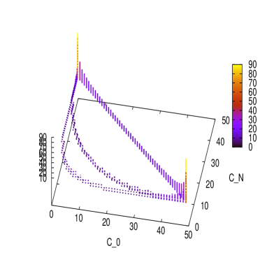
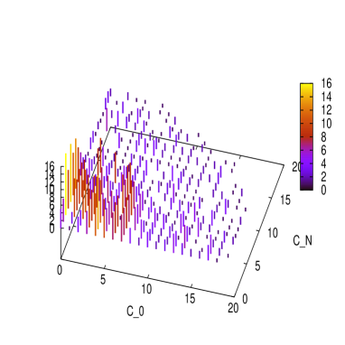
Figure 4: Probability $P(c_{0},c_{N})$ for creating a N00N state in coupled harmonic cavities with $N=2,4,6$ (from right to left in the left panel) and in coupled anharmonic cavities with $N=100$ (right panel). The parameters are the same as in the previous Figure.

V Discussion and Conclusions

We have considered a pair of optical cavities, where the photons in each cavity couple to a two-level atom. Then the cavities are described as JC models. For the initial state both cavities are prepared in an eigenstate of the JC Hamiltonian. Then we have connected the cavities by an optical fiber such that photons can tunnel between them. The resulting evolution of the quantum state of the combined system is determined by an effective Hamiltonian that resembles the Bose-Hubbard model with modified photon-photon interaction. The cavity frequency $\omega_{0}$ is assumed to be the same in both cavities. In this case $\omega_{0}$ provides only a global shift of the spectrum, whereas the level spacing is entirely determined by the tunneling rate $J$ of the optical fiber. For harmonic cavities (i.e. in the absence of the two-level atoms) the distribution of the levels with spectral weights $p_{j}=|\langle\Psi_{0}|E_{j}\rangle|^{2}$ is binomial with equidistant energy levels. The resulting evolution is periodic and corresponds to Rabi oscillations with a single frequency $J$. This behavior was observed experimentally for weakly interacting bosonic atoms ketterle04 ; oberthaler05 and should also be accessible for photons in harmonic cavities. The amplitudes for visiting the initial Fock state $|N,0\rangle$ or the complimentary Fock state $|0,N\rangle$ vary as $\cos^{N}(Jt)$ or $(-i)^{N}\sin^{N}(Jt)$, respectively. This implies for a large number $N$ of bosons that (i) these states are visited only for a very short period of time and (ii) the two Fock states are visited at different times. Thus the dynamical creation of a N00N state from a Fock state $|N,0\rangle$ is very unlikely for harmonic cavities, unless the number of photons is small. The reason is that the photons can travel without seeing each other through the entire Hilbert space. A simultaneous overlap of $|\Psi_{t}\rangle$ with both Fock states $|N,0\rangle$ and $|0,N\rangle$ is very unlikely then. This is a situation in which it is very difficult to control and follow the quantum evolution. On the other hand, applications of finite quantum systems, such as in quantum information processing garcia05 ; wineland11 , require a controllable evolution, in which only certain parts of the available Hilbert space can be visited with reasonable probability. In terms of our two-cavity system this means that the spectral weight $p_{j}=|\langle\Psi_{0}|E_{j}\rangle|^{2}$ with respect to the initial state $|\Psi_{0}\rangle$ is small for most eigenstates $|E_{j}\rangle$ and has only a few pronounced maxima that can be used for information storage. We have found that such a structured spectral density appears for anharmonic cavities, created by coupling two-level atoms to the cavity photons. Then the photons experience a mutual influence which restricts their individual random walks in Hilbert space significantly and, what is even more important here, they can have a simultaneous overlap with both states $|0,N\rangle$ and $|0,N\rangle$. This effect enables the system to create dynamically a N00N state. The latter allows us to conclude that the complex quantum dynamics of two coupled anharmonic optical cavities offers an approach for quantum information processing as it has also been proposed for ultracold atoms garcia05 and cold trapped ions wineland11 .

References

- (1) I. Bloch, Science 319, 202 (2008).
- (2) V.I. Yukalov, Laser Phys. 19, 1 (2009).
- (3) S. Trotzky, P. Cheinet, S. Folling, M. Feld, U. Schnorrberger, A. M. Rey, A. Polkovnikov, E. A. Demler, M. D. Lukin, and I. Bloch Science, 319, 295 (2008).
- (4) Y. Shin, M. Saba, A. Schirotzek, T.A. Pasquini, A.E. Leanhardt, D.E. Pritchard, and W. Ketterle, Phys. Rev. Lett. 92, 150401 (2004).
- (5) M. Albiez, R. Gati, J. Fölling, S. Hunsmann, M. Cristiani, and M.K. Oberthaler, Phys. Rev. Lett. 95, 010402 (2005).
- (6) C. Kollath, A.M Läuchli, and E. Altman, Phys. Rev. Lett. 98, 180601 (2007).
- (7) M. Rigol, V. Dunjko, V. Yurovsky, and M. Olshanii, Phys. Rev. Lett. 98, 050405 (2007).
- (8) S.R. Manmana, S. Wessel, R.M. Noack, and A. Muramatsu, Phys. Rev. Lett. 98, 210405 (2007).
- (9) M. Eckstein and M. Kollar, Phys. Rev. Lett. 100, 120404 (2008).
- (10) M. Kollar and M. Eckstein, Phys. Rev. A 78, 013626 (2008).
- (11) M. Möckel and S. Kehrein, Phys. Rev. Lett. 100, 175702 (2008).
- (12) V.I. Yukalov, Laser Phys. Lett. 8, No. 7, 485 (2011).
- (13) V.I. Yukalov, A. Rakhimov and S. Mardonov, Laser Phys. 21, 264 (2011).
- (14) G. Roux, Phys. Rev. A 79, 021608 (2009).
- (15) M. Rigol, Phys. Rev. A 82, 037601 (2010).
- (16) M. Brune, J. Bernu, C. Guerlin, S. Deléglise, C. Sayrin, S. Gleyzes, S. Kuhr, I. Dotsenko, J.M. Raimond, and S. Haroche, Phys. Rev. Lett. 101, 240402 (2008).
- (17) H. Wang, M. Hofheinz, M. Ansmann, R.C. Bialczak, E. Lucero, M. Neeley, A.D. O Connell, D. Sank, J. Wenner, A.N. Cleland, and John M. Martinis, Phys. Rev. Lett. 101, 240401 (2008).
- (18) H. Carmichael, Nature Phys. 4, 346 (2008).
- (19) I. Schuster, A. Kubanek, A. Fuhrmanek, T. Puppe, P.H.W. Pinske, K. Murr and G. Rempe, Nature Phys. 4, 382 (2008).
- (20) K. Ziegler, Laser Physics 22, 331 (2012).
- (21) A. Imamoglu, H. Schmidt, G. Woods, and M. Deutsch, Phys. Rev. Lett. 79, 1467 (1997).
- (22) P. Grangier, D.F. Walls and K.M. Gheri, Phys. Rev. Lett. 81, 2833 (1998).
- (23) M.J. Hartmann, F.G.S.L. Brandão and M.B. Plenio, Nature Phys. 2, 849 (2006).
- (24) M.J. Hartmann, F.G.S.L. Brandão and M.B. Plenio, Laser & Photon. Rev. 2, 527556 (2008).
- (25) A.-C. Ji, Q. Sun, X.C. Xie, and W.M. Liu, Phys. Rev. Lett. 102, 023602 (2009).
- (26) H. Lee, P. Kok and J.P. Dowling, Journal of Modern Optics 49, 2325 (2002).
- (27) P. Walther, J.-W. Pan, M. Aspelmeyer, R. Ursin, S. Gasparoni and A. Zeilinger, Nature 429, 158 (2004).
- (28) M.W. Mitchell, J.S. Lundeen and A. M. Steinberg, Nature 429, 161 (2004).
- (29) I. Afek, O. Ambar and Y. Silberberg, Science 328, 879 (2010).
- (30) A. Boto, P. Kok, Phys. Rev. Lett. 99 2733 (2000).
- (31) P. Kok, H. Lee and J.P. Dowling, Phys. Rev. 65, 052104 (2002).
- (32) H. Cable and J.P. Dowling, Phys. Rev. Lett. 99, 163604 (2007).
- (33) K. Ziegler, J. Phys. B: At. Mol. Opt. Phys. 44, 145302 (2011).
- (34) E.T. Jaynes and F.W. Cummings, Proc. Inst. Elect. Eng. 51, 89 (1963).
- (35) F.W. Cummings, Phys. Rev. 140, A1051 (1965).
- (36) K. Ziegler, Phys. Rev. A 81, 034701 (2010).
- (37) D. Kleppner, Phys. Rev. Lett. 47, 233 (1981).
- (38) R.R. Puri and G.S. Argawal, Phys. Rev. A 33 3610 (1985).
- (39) V. Buzek and I. Jex, J. Mod. Optics 36, 1427 (1989).
- (40) M. Cramer, C.M. Dawson, J. Eisert, and T.J. Osborne, Phys. Rev. Lett. 100, 030602 (2008).
- (41) J.J. Garc a-Ripoll, P. Zoller, and J.I. Cirac, J. Phys. B: At. Mol. Opt. Phys. 38, S567 (2005).
- (42) D.J. Wineland and D. Leibfried, Laser Phys. Lett. 8, Issue 3, 175 (2011).