Generalized Effective Potential Landau Theory for Bosonic Superlattices

Abstract

We study the properties of the Bose-Hubbard model for square and cubic superlattices. To this end we generalize a recently established effective potential Landau theory for a single component to the case of multi components and find not only the characteristic incompressible solid phases with fractional filling, but also obtain the underlying quantum phase diagram in the whole parameter region at zero temperature. Comparing our analytic results with corresponding ones from quantum Monte Carlo simulations demonstrates the high accuracy of the generalized effective potential Landau theory (GEPLT). Finally, we comment on the advantages and disadvantages of the GEPLT in view of a direct comparison with a corresponding decoupled mean-field theory.

I Introduction

Systems of ultracold bosonic gases in optical lattices have recently become a major field in physics research Lewenstein:AdP07 ; Bloch:RMP08 ; Sanpera . After their theoretical suggestion Fisher:PRB89 ; Jaksch:PRL98 and first experimental realization using counter-propagating laser beams Greiner:Nat02 it soon became clear that they establish a versatile bridge between the field of ultracold quantum matter and correlated condensed matter systems Bloch:NaP12 .

One of the most famous examples is the Bose-Hubbard model Fisher:PRB89 ; Jaksch:PRL98 which undergoes a quantum phase transition from a Mott insulator to a superfluid phase due to the competition between the atom-atom on-site interaction and the hopping amplitude. This transition can be demonstrated experimentally by time-of-flight absorption pictures Greiner:Nat02 , or measuring the collective excitation spectra via Bragg spectroscopy sengstock1 ; sengstock2 . Recent research efforts have targeted more complex systems, which include long-range interactions (e.g. from dipolar bosons Fleischhauer1 ; bloch:na12 ), mixtures of several components Hofstetter1 ; sengstock3 and more interesting lattice geometries, such as frustrated or superlattice structures experiment1 ; experiment2 ; experiment4 ; experiment3 ; experiment5 . Accordingly, the corresponding phase diagrams become richer and more complex, including the possibility of phases with periodic density modulations or supersolidity. A crystalline density wave phase, for instance, generally occurs at fractional filling and it has been proposed that the corresponding commensurate density modulation could be detected by measuring correlations with time-of-flight and noise-correlation techniques hou . Furthermore, recent experimental progress in achieving single-site addressability in optical lattice structures ss1 ; ss2 ; ss3 ; ss4 ; ss5 ; ss6 ; ss7 nourishes the prospect to directly observe density wave modulations in the near future.

Such density modulations may emerge from interactions via spontaneous symmetry-breaking, but a a simpler way to create them is with a superlattice generated from commensurate lasers, see for instance Refs. experiment1 ; experiment2 ; experiment4 ; experiment3 ; experiment5 for further experimental details. Thus, then the potential depth is slightly different on one sublattice, while the interaction strength and hopping amplitude will remain almost uniform. The corresponding Bose-Hubbard model Hamiltonian on a square or cubic lattice is given by vezzani

$$\hat{H}_{\rm SL}=-t\sum_{\langle j\in A,j^{\prime}\in B\rangle}\left(\hat{a}_{j}^{{\dagger}}\hat{a}_{j^{\prime}}^{\phantom{{\dagger}}}+\hat{a}_{j}^{\phantom{{\dagger}}}\hat{a}_{j^{\prime}}^{{\dagger}}\right)$$ (1)

$$+\frac{U}{2}\sum_{j\in A,B}\hat{n}_{j}\left(\hat{n}_{j}-1\right)-\left(\mu+\Delta\mu\right)\sum_{j\in A}\hat{n}_{j}-\mu\sum_{j\in B}\hat{n}_{j}\,,$$

where $\Delta\mu$ stands for a small additional chemical potential on sublattice $A$ compared to sublattice B, as illustrated in Fig. 1. As we will show this model exhibits an interesting competition between Mott and density wave phases.

From a theoretical point of view the study of interacting bosons and quantum phase transitions is far from trivial Sachdev . The possible phases in different kinds of optical superlattices have so far been analyzed by numerical approaches scalettar ; schollwoeck ; das2 , decoupled mean field theory vezzani ; hou ; shuchen ; das1 , multisite mean-field theory msmf1 ; msmf2 ; msmf3 ; msmf4 and cell strong-coupling expansion method csce1 ; csce2 . The latter method yields excellent results for $1$d systems when compared to the powerful numerical method of Ref. msmf3 . However, it is known that mean-field theory can have significant deviations from unbiased high-precision numerical results zhang and the strong-coupling expansion is not that accurate when applied to higher dimensional systems. The purpose of this paper is, therefore, to present a reliable quantitative method to determine non-trivial phases of high-dimensional multi-component boson systems. To this end we profit from recent advances to use a systematic Landau theory with an effective potential that can be estimated quantitatively from the microscopic model, e.g. by diagrammatic methods pelster1 ; pelster2 ; pelster3 ; pelster4 ; jiangying ; pelster5 . Whereas the first hopping order of the effective potential Landau theory leads to similar results as mean-field theory Fisher:PRB89 , higher hopping orders have recently been evaluated via the process-chain approach Eckardt ; Holthaus5 ; Holthaus6 ; Teichmann ; Holthaus7 , which determines the location of the quantum phase transition for the single component Hubbard model for cubic as well as triangular and hexagonal optical lattices to a similar precision as demanding quantum Monte Carlo simulations MC1 ; MC2 . Thus, it becomes even possible to calculate the critical exponents of the corresponding quantum phase transition exponents1 ; exponents2 . We now present a generalized effective potential Landau theory (GEPLT), which extends those concepts to multi-component systems and to phases with non-trivial crystalline order parameters. In particular, for the model in Eq. (1) the GEPLT approach gives excellent quantitative estimates for the location of the phase boundaries compared to unbiased quantum Monte Carlo simulations.

At first, we briefly review the effective potential Landau theory for the single component Bose-Hubbard model in Sec. II. Then, we extend this method step by step from one component to the general superlattice case in Section III. After that, we apply this GEPLT method to the simple superlattice model in Eq. (1) and determine the resulting quantum phase diagram at zero temperature in the whole parameter region in Section IV. Both the advantages and disadvantages of GEPLT are revealed by comparing it with a decoupled mean-field theory in Section V. Finally, Section VI provides the conclusions and sketches related problems in an outlook.

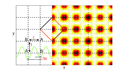
Figure 1: (Color online) Schematic illustration for a square superlattice in two dimensions. The solid line square represents one type of the unit cell. The solid curve (green) shows the optical potential in the $x$ direction. Lattice sites $A$ are deeper by $\Delta\mu$ than lattice sites $B$.

II Effective Potential Landau Theory

Let us first consider the Bose Hubbard model in Eq. (1) for the well-studied case of $\Delta\mu=0$ Fisher:PRB89 ; Jaksch:PRL98 . The second-order quantum phase transition between the Mott insulator, which occurs for $t/U\ll 1$, and the superfluid, which is realized for $t/U\gg 1$, is intimately connected with a spontaneous breaking of the underlying U(1)-symmetry of the Bose-Hubbard model (1). To describe this theoretically, we transfer the usual field-theoretic approach for thermal phase transitions Zinn-Justin ; Kleinert to quantum phase transitions and couple the creation and annihilation operators to external source fields with uniform strength $J$ and $J^{*}$ within a Landau theory pelster2 ; pelster3

$$\hat{H}_{\rm BH}(J,J^{*})=\hat{H}_{\rm BH}+\sum_{j}\left(J\hat{a}_{j}^{{\dagger}}+J^{*}\hat{a}_{j}\right)\,.$$ (2)

The transition from the Mott insulator to the superfluid phase is described by the emergence of a non-vanishing order parameter which is defined due to homogeneity according to $\psi=\langle\hat{a}_{i}\rangle$, $\psi^{*}=\langle\hat{a}_{i}^{{\dagger}}\rangle$. The free energy corresponding to (2)

$$F(J,J^{*})=-\frac{1}{\beta}\,\ln\left[\mbox{Tr}\,e^{-\beta\hat{H}_{\rm BH}(J,J^{*})}\right]$$ (3)

allows to determine this order parameter via

$$\psi=\frac{1}{N_{s}}\frac{\partial F(J,J^{*})}{\partial J^{*}}\,,\quad\psi^{*}=\frac{1}{N_{s}}\frac{\partial F(J,J^{*})}{\partial J}\,,$$ (4)

where $N_{s}$ denotes the number of lattice sites. Equation (4) motivates that it is possible to formally perform a Legendre transformation from the free energy $F(J,J^{*})$ in order to arrive at an effective potential $\Gamma(\psi,\psi^{*})$ that is useful in a quantitative Landau theory

$$\Gamma(\psi,\psi^{*})=F/N_{s}-\psi^{*}J-\psi J^{*}\,.$$ (5)

Due to Legendre identities the external sources can be reobtained from derivatives of the effective potential

$$\frac{\partial\Gamma}{\partial\psi^{*}}=-J,\quad\frac{\partial\Gamma}{\partial\psi}=-J^{*}\,.$$ (6)

The original Bose-Hubbard Hamiltonian (1) is restored from (2) for vanishing currents, i.e. by setting $J=J^{*}=0$. In this limit we conclude from (5) that the effective potential reduces to the free energy. Furthermore, Eq. (6) then implies that the order parameter $\psi,\psi^{*}$ of the system follows from extremizing the effective potential. A trivial extremum $\psi=0$ corresponds to the Mott-insulator phase, whereas a non-vanishing extremum $\psi\neq 0$ occurs in the superfluid phase.

The free energy (2) reduces at zero temperature to the ground-state energy, which can be calculated in a power series of both the hopping parameter $t$ and the source terms $J,J^{*}$ by using the Rayleigh-Schrödinger perturbation theory pelster1 ; pelster2 ; pelster3 ; pelster4 ; jiangying ; pelster5 ; Eckardt ; Holthaus5 ; Holthaus6 ; Teichmann ; Holthaus7 . Due to the underlying U(1)-symmetry of the Bose-Hubbard Hamiltonian (1) the expansion is only a power series in terms of $|J|^{2}$

$$F(J,J^{*},t)=N_{s}\left(F_{0}(t)+\sum_{p=1}^{\infty}c_{2p}(t)\left|J\right|^{2p}\right)\,,$$ (7)

where the respective expansion coefficients are accessible via a hopping expansion

$$c_{2p}(t)=\sum_{n=0}^{\infty}(-t)^{2n}\alpha_{2p}^{(n)}\,.$$ (8)

From Eqs. (4), (6), and (7) we then obtain the effective potential of the Bose-Hubbard Hamiltonian (1) in the following perturbative form

$$\Gamma(\psi,\psi^{*},t)=F_{0}(t)-\frac{1}{c_{2}(t)}|\psi|^{2}+\frac{c_{4}(t)}{c_{2}(t)^{4}}|\psi|^{4}+\cdots\,.$$ (9)

According to the Landau theory for second-order phase transitions, the critical line between the Mott insulator and the superfluid phase follows from finding the zero of the second-order coefficient in (9). In order to solve the resulting equation $1/c_{2}(t_{c})=0$, we expand it in a power series of the hopping parameter $t$

$$\frac{1}{c_{2}(t)} = \frac{1}{\alpha_{2}^{(0)}}\left(1+\frac{\alpha_{2}^{(1)}}{\alpha_{2}^{(0)}}t+\left[\left(\frac{\alpha_{2}^{(1)}}{\alpha_{2}^{(0)}}\right)^{2}-\frac{\alpha_{2}^{(2)}}{\alpha_{2}^{(0)}}\right]t^{2}\right.$$ (10)

$$+\cdots\Big{)}\,.$$

Thus this gives us an algebraic equation for $t_{c}$, whose degree depends on the respective hopping order which is taken into account. The number of the roots is the same as the order of $t$, but only the smallest real positive root is identified as an appropriate approximation for the location of the quantum phase transition.

As mentioned in the introduction, the effective potential Landau theory was quite successful in calculating the quantum phase boundary for the single component system pelster1 ; pelster2 ; pelster3 ; pelster4 ; jiangying ; pelster5 ; Eckardt ; Holthaus5 ; Holthaus6 ; Teichmann ; Holthaus7 . However, it cannot be used to treat a superlattice system, since more than one order parameter appears. Therefore, we will work out in the next section a corresponding extension to multi components which overcomes this problem.

III Generalized Effective Potential Landau Theory

In order to describe a superlattice or a multi-component system, we have to introduce several sites or degrees of freedom at each lattice point. In other words, we introduce a larger unit cell at each lattice point, labeled by $j$, together with a basis of size $m$, labeled by $l=1,..,m$. The generalized Bose-Hubbard Hamiltonian with $m$ bosonic species in each unit cell is therefore given by

$$\hat{H}_{\rm BH} = -\sum_{j,j^{\prime}}\sum_{l,l^{\prime}=1}^{m}\left[t_{j(l),j^{\prime}(l^{\prime})}\hat{a}_{j(l)}^{\dagger}\hat{a}_{j^{\prime}(l^{\prime})}^{\phantom{{\dagger}}}+\mbox{h.c.}\right]$$

$$+\sum_{j}\sum_{l=1}^{m}\left[\frac{U_{(l)}}{2}\hat{n}_{j(l)}\left(\hat{n}_{j(l)}-1\right)-\mu_{(l)}\hat{n}_{j{(l)}}\right]\,,$$

where $\hat{a}_{j(l)}$ denotes the boson annihilation operator at lattice point $j$ with basis index $(l)$. Hopping $t_{j(l),j^{\prime}(l^{\prime})}$ can occur between any basis and lattice position, while the repulsion $U_{(l)}$ acts for now only between bosons of the same lattice point and basis index. The chemical potential $\mu_{(l)}$ depends on the basis index which is analogous to sublattices $A$ and $B$ in Eq. (1).

We now model the symmetry-breaking by introducing the source vectors $\vec{\mathbb{J}}=(J_{1},\ldots,J_{m})^{\rm T},\vec{\mathbb{J}}^{{\dagger}}=(J_{1}^{*},\ldots,J_{m}^{*})$ according to

$$\hat{H}_{\rm BH}(\vec{\mathbb{J}},\vec{\mathbb{J}}^{{\dagger}})=\hat{H}_{\rm BH}+\sum_{j}\sum_{l=1}^{m}\left(J_{l}^{\phantom{*}}\hat{a}_{j{(l)}}^{\dagger}+J_{l}^{*}\hat{a}_{j{(l)}}^{\phantom{{\dagger}}}\right)\,.$$ (12)

By generalizing the procedure from a single component to multi components, we use perturbation theory in order to determine the free energy at zero temperature in a power series of both the hopping parameters $t_{j{(l)},j^{\prime}{(l^{\prime})}}$ and the source vectors $\vec{\mathbb{J}},\vec{\mathbb{J}}^{{\dagger}}$. In principle, we need an expansion in terms of all relevant hopping parameters $t_{j{(l)},j^{\prime}{(l^{\prime})}}$, but to illustrate the process we consider here the case that only one hopping element $t$ dominates (e.g. between nearest neighbors) and all others are neglected

$$F(\vec{\mathbb{J}},\vec{\mathbb{J}}^{{\dagger}},t)=N_{s}\Big{[}F_{0}(t)+\vec{\mathbb{J}}^{{\dagger}}C_{2}(t)\vec{\mathbb{J}}+\cdots\Big{]}\,.$$ (13)

The matrix elements $c_{2ll^{\prime}}^{\phantom{(n)}}(t)$ of $C_{2}(t)$ are then given by a hopping expansion of the form

$$c_{2ll^{\prime}}^{\phantom{(n)}}(t)=\sum_{n=0}^{\infty}\left(-t\right)^{n}\alpha_{2ll^{\prime}}^{(n)}\,.$$ (14)

The order parameter vectors give different values for each basis index, but are independent of lattice points $\vec{\Psi}=(\psi_{1},\ldots,\psi_{m})^{\rm T},\vec{\Psi}^{{\dagger}}=(\psi_{1}^{*},\ldots,\psi_{m}^{*})$ according to

$$\vec{\Psi} = \left(\langle\hat{a}_{1}\rangle,\ldots,\langle\hat{a}_{m}\rangle\right)^{\rm T}\,,$$

$$\vec{\Psi}^{{\dagger}} = \left(\langle\hat{a}_{1}^{{\dagger}}\rangle,\ldots,\langle\hat{a}_{m}^{{\dagger}}\rangle\right)\,,$$ (15)

and we observe

$$\psi_{i}=\frac{1}{N_{s}}\frac{\partial F}{\partial J^{*}_{i}}\,,\quad\psi_{i}^{*}=\frac{1}{N_{s}}\frac{\partial F}{\partial J_{i}}\,.$$ (16)

Again this motivates to perform the Legendre transformation of the free energy. The generalized effective potential then depends on the order parameter vectors $\vec{\Psi},\vec{\Psi}^{{\dagger}}$:

$$\Gamma(\vec{\Psi},\vec{\Psi}^{{\dagger}},t)=F/N_{s}-\vec{\mathbb{J}}^{{\dagger}}\vec{\Psi}-\vec{\Psi}^{{\dagger}}\vec{\mathbb{J}}\,.$$ (17)

Legendre identities allow to write the external sources as derivatives of the effective potential

$$\frac{\partial\Gamma}{\partial\psi_{i}}=-J_{i}^{*}\,,\quad\frac{\partial\Gamma}{\partial\psi_{i}^{*}}=-J_{i}\,,$$ (18)

so the order parameter vector is determined by extremizing $\Gamma$ in the physical limit that the external source vectors $\vec{\mathbb{J}},\vec{\mathbb{J}}^{{\dagger}}$ vanish.

Due to Eqs. (13), (16), and (17) the effective potential of the system is of the form

$$\Gamma(\vec{\Psi},\vec{\Psi}^{{\dagger}},t)=F_{0}(t)+\vec{\Psi}^{{\dagger}}A_{2}(t)\vec{\Psi}+\cdots\,.$$ (19)

The resulting relation between the matrices $A_{2}$ and $C_{2}$ can be deduced in following way. By inserting (19) into (18), we get

$$A_{2.ij}=\frac{\partial^{2}\Gamma}{\partial\psi_{i}^{*}\partial\psi_{j}}=-\frac{\partial J_{i}}{\partial\psi_{j}}\,.$$ (20)

Combining this with (13) and (16), we read off

$$-\delta_{ij}=A_{2,ik}\frac{\partial\psi_{k}}{\partial J_{j}}=\frac{1}{N_{s}}A_{2,ik}\frac{\partial^{2}F}{\partial J_{k}^{*}\partial J_{j}}=\left(A_{2}C_{2}\right)_{ij}\,.$$ (21)

Thus, the matrix $A_{2}$ turns out to be the inverse of $-C_{2}$. As all matrix elements of $C_{2}$ are given by a hopping expansion of the form (14), we get a corresponding hopping expansion for each element of $A_{2}$. In matrix form the first terms of this hopping expansion read

$$C_{2}^{-1}=\left(\alpha_{2}^{(0)}\right)^{-1}\left\{1+\alpha_{2}^{(1)}\left(\alpha_{2}^{(0)}\right)^{-1}t+\left[\alpha_{2}^{(1)}\left(\alpha_{2}^{(0)}\right)^{-1}\right.\right.$$

$$\left.\left.\alpha_{2}^{(1)}\left(\alpha_{2}^{(0)}\right)^{-1}+\alpha_{2}^{(2)}\left(\alpha_{2}^{(0)}\right)^{-1}\right]t^{2}+...\right\}\,,$$ (22)

which reduces for a single component to (10). The critical line, where the order parameter vector $\vec{\Psi}$ changes from zero to non-zero, follows then from extremizing the effective potential (19). In case that all components of the order parameter vector $\vec{\Psi}$ are non-zero, we obtain

$$\mbox{Det}\,A_{2}=0\,.$$ (23)

But it could also happen that only a subset of components of the order parameter vector $\vec{\Psi}$ is non-vanishing, which yields the condition that the determinant of the corresponding submatrix of $A_{2}$ vanishes. The physically realized quantum phase boundary corresponds then to the smallest value of the hopping parameter $t$, which follows from all these conditions. In the next section we will study along these lines the most simple case of a superlattice system which is provided by bosons on a square or cubic superlattice given in Eq. (1).

IV Square and Cubic Superlattice

Similar to the continuous translational symmetry breaking artificially introduced by the optical lattice to mimic a real crystal, the optical superlattice can break the discrete translational symmetry to study the multi-components system. Beside that, it also can be used as a platform for disorder disorder and topological order TI1 ; TI2 problems. Here, we apply the GEPLT to the simple square and cubic case.

IV.1 Application of Effective Potential Theory

Following the GEPLT from the previous section for the model in Eq. (1) we need to use for the two sublattices two independent source terms $\vec{\mathbb{J}}=(J_{A},J_{B})^{\rm T}$, yielding

$$\hat{H}_{\rm SL}(\vec{\mathbb{J}},\vec{\mathbb{J}}^{{\dagger}}) = \hat{H}_{\rm SL}+\sum_{j\in A}\left(J_{A}\hat{a}_{j}^{{\dagger}}+J_{A}^{*}\hat{a}_{j}^{\phantom{{\dagger}}}\right)$$ (24)

$$+\sum_{j\in B}\left(J_{B}\hat{a}_{j}^{{\dagger}}+J_{B}^{*}\hat{a}_{j}^{\phantom{{\dagger}}}\right)\,.$$

The free energy of the system can then be written as (13), where $C_{2}(t)$ represents a 2x2-matrix with the following hopping expansion

$$\left(\begin{array}[]{cc}c_{2AA}&c_{2AB}\\ c_{2BA}&c_{2BB}\\ \end{array}\right)=\sum_{n=0}^{\infty}\left(-t\right)^{n}\left(\begin{array}[]{cc}\alpha_{2AA}^{(n)}&\alpha_{2AB}^{(n)}\\[2.84526pt] \alpha_{2BA}^{(n)}&\alpha_{2BB}^{(n)}\\ \end{array}\right)\,,$$ (29)

where the symmetry $c_{2AB}=c_{2BA}$ holds. Then, after the Legendre transformation (17), we obtain the effective potential (19), where we have $\vec{\Psi}=(\langle\hat{a}_{A}\rangle,\langle\hat{a}_{B}\rangle)^{\rm T}$ and $A_{2}$ is the inverse of $-C_{2}$ according to Eq. (21). When the second-order quantum phase transition occurs, the vanishing order parameter vector $\vec{\Psi}=(0,0)^{\rm T}$ changes from stable to unstable. It turns out that the smallest critical hopping parameter results from the condition (23) that the determinant of $A_{2}$ vanishes. With this we obtain in second order of $t$ the following equation for the location of the quantum phase boundary

$$(\beta^{(0)})^{2}-\beta^{(0)}\beta^{(1)}t-\frac{\beta^{(2)}t^{2}}{2}=0\,,$$ (30)

where the abbreviations $\beta^{(0)}=\sqrt{\alpha_{2AA}^{(0)}\alpha_{2BB}^{(0)}}$, $\beta^{(1)}=\alpha_{2AB}^{(1)}$, and $\beta^{(2)}=\alpha_{2AA}^{(2)}\alpha_{2BB}^{(0)}+\alpha_{2AA}^{(0)}\alpha_{2BB}^{(2)}-2(\alpha_{2AB}^{(1)})^{2}$ have been introduced. Taking into account the smallest root then yields

$$t_{c}=\frac{\beta^{(0)}\left[-\beta^{(1)}+\sqrt{(\beta^{(1)})^{2}+2\beta^{(2)}\,}\right]}{\beta^{(2)}}\,.$$ (31)

Thus, the problem of finding the quantum phase boundary has been reduced to the calculation of the perturbative coefficients $\alpha_{2ll^{\prime}}^{(n)}$ in the respective hopping order. According to Appendix A this perturbative calculation can be systematically performed by using a suitable diagrammatic representation. We use the unperturbed energies

$$E^{(0)}\left(n_{A},n_{B}\right) = \frac{U}{2}n_{A}\left(n_{A}-1\right)+\frac{U}{2}n_{B}\left(n_{B}-1\right)$$ (32)

$$-\left(\mu+\Delta\mu\right)n_{A}-\mu n_{B}\,,$$

to define the energy differences between different particle number sectors

$$\lambda_{A}^{\pm(p)}= \left[E^{(0)}\left(n_{A},n_{B}\right)-E^{(0)}\left(n_{A}\pm p,n_{B}\right)\right]/N_{s},$$

$$\lambda_{B}^{\pm(p)}= \left[E^{(0)}\left(n_{A},n_{B}\right)-E^{(0)}\left(n_{A},n_{B}\pm p\right)\right]/N_{s}.$$ (33)

For $p=\pm 1$ the short notation $\lambda_{A}^{\pm}=\lambda_{A}^{\pm(1)}$, $\lambda_{B}^{\pm}=\lambda_{B}^{\pm(1)}$ is used. In zeroth and first hopping order we obtain the following results for the respective coefficients $\alpha^{(n)}_{2ll^{\prime}}$

$$\alpha_{2AA(BB)}^{(0)}=\frac{n_{A(B)}+1}{\lambda_{A(B)}^{+}}+\frac{n_{A(B)}}{\lambda_{A(B)}^{-}}$$ (34)

$$\alpha_{2AB}^{(1)}=\alpha_{2BA}^{(1)}=z\alpha_{2AA}^{(0)}\alpha_{2BB}^{(0)}\,,$$ (35)

whereas in second hopping order we get

$$\alpha_{2AA}^{(2)}=z(z-1)(\alpha_{2AA}^{(0)})^{2}\alpha_{2BB}^{(0)}+z\left[\frac{n_{A}^{2}n_{B}}{{\left(\lambda_{A}^{-}\right)^{2}\lambda_{B}^{-}}}\right.$$

$$+\frac{n_{A}n_{B}\left(1+n_{A}\right)}{\lambda_{A}^{-}\left(\lambda_{A}^{+}+\lambda_{B}^{-}\right)}\left(\frac{2}{\lambda_{B}^{-}}-\frac{1}{\lambda_{A}^{+}+\lambda_{B}^{-}}-\frac{1}{\lambda_{A}^{-}}\right)$$

$$+\frac{n_{A}\left(1+n_{A}\right)\left(1+n_{B}\right)}{\lambda_{A}^{+}\left(\lambda_{A}^{-}+\lambda_{B}^{+}\right)}\left(\frac{2}{\lambda_{B}^{+}}-\frac{1}{\lambda_{A}^{-}+\lambda_{B}^{+}}-\frac{1}{\lambda_{A}^{+}}\right)$$

$$+\frac{n_{B}(n_{A}+1)^{2}}{\lambda_{A}^{+}+\lambda_{B}^{-}}\left(\frac{\lambda_{A}^{+}-\lambda_{B}^{-}}{\lambda_{A}^{+}\lambda_{B}^{-}\left(\lambda_{A}^{+}+\lambda_{B}^{-}\right)}-\frac{1}{(\lambda_{A}^{+})^{2}}\right)$$

$$+\frac{n_{A}^{2}\left(1+n_{B}\right)}{\lambda_{A}^{-}+\lambda_{B}^{+}}\left(\frac{\lambda_{A}^{-}-\lambda_{B}^{+}}{\lambda_{A}^{-}\lambda_{B}^{+}\left(\lambda_{A}^{-}+\lambda_{B}^{+}\right)}-\frac{1}{\left(\lambda_{A}^{-}\right)^{2}}\right)$$

$$+\frac{\left(1+n_{A}\right)\left(2+n_{A}\right)n_{B}}{\lambda_{A}^{+(2)}+\lambda_{B}^{-}}\left(\frac{1}{\lambda_{A}^{+}}+\frac{1}{\lambda_{A}^{+}+\lambda_{B}^{-}}\right)^{2}$$

$$+\frac{\left(n_{A}-1\right)\left(1+n_{B}\right)n_{A}}{\lambda_{A}^{-(2)}+\lambda_{B}^{+}}\left(\frac{1}{\lambda_{A}^{-}}+\frac{1}{\lambda_{A}^{-}+\lambda_{B}^{+}}\right)^{2}$$

$$\left.+\frac{\left(1+n_{A}\right)^{2}\left(1+n_{B}\right)}{\left(\lambda_{A}^{+}\right)^{2}\lambda_{B}^{+}}\right]\,$$ (36)

and analogous for $\alpha_{2BB}^{(2)}$ with the indices $A$ and $B$ interchanged.

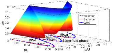
Figure 2: (Color online) The quantum phase diagram of a bosonic 2$d$ square superlattice in the whole parameter region from first hopping order GEPLT, and the phase diagram projected in the $t$-$\mu$ plane comparing the quantum Monte Carlo simulation (dotted line), the 1st order (dashed line) and the 2nd order (solid line) analytic results at $\Delta\mu/U=0.5$.

IV.2 Quantum Phase Diagram

In order to got the whole quantum phase diagram, we study at first the $t=0$ contribution of the effective potential in Eq. (19), i.e. $F_{0}(t=0)=N_{s}E^{(0)}\left(n_{A},n_{B}\right)$ with Eq. (32). We assume $\Delta\mu$ to be in the region of $[0,U)$. Similar to the normal Bose-Hubbard model, there exist Mott insulator phases (Mott-$n$), which are characterized by the uniform filling $n_{A}=n_{B}=n$. However, due to the local offset $\Delta\mu$, this happens only in the regions

$$\mbox{Mott-$n$:}\quad U\left(n-1\right)<\mu<Un-\Delta\mu\,.$$ (37)

On the other hand the density wave phases (DW-$n$) break the translational order as they have the property $n_{B}=n_{A}-1$, $n_{A}=n$, yielding the filling factor $n+1/2$, and minimize the free energy in the other regions

$$\mbox{DW-$n$:}\quad(n-1)U-\Delta\mu<\mu<(n-1)U\,.$$ (38)

Hence, depending on the chemical potential offset $\Delta\mu$, we find a natural competition between Mott phases and density wave phases.

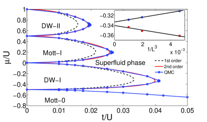
Figure 3: (Color online) The quantum phase boundaries of a bosonic 3$d$ cubic superlattice at $\Delta\mu/U=0.5$ which is obtained by 1st order (dashed line) and 2nd order (solid line) generalized effective Landau potential theory, and the quantum Monte Carlo simulation (dotted line) in the thermodynamic limit. Inset: Finite-size scaling of the critical points of DW-I at $t/U=0.04125$.

Turning on the hopping processes, the quantum fluctuations will melt the different insulating phases, and the critical lines are determined in second hopping order by Eq. (31) after substituting the respective strong-coupling coefficients $\alpha^{(n)}_{2ll^{\prime}}$ from Eqs. (34)–(36). The resulting quantum phase diagram for square and cubic superlattices are shown in Fig. 2 and Fig. 3, respectively.

From the GEPLT calculation we find for the special case $\Delta\mu=0$ that the Mott-1 lobe coincides with the single component method from Ref. [pelster2, ] as expected. In addition, when $\Delta\mu$ is larger than zero, the DW phase appears, and its region increases with increasing $\Delta\mu$, whereas the region of the Mott phase decreases correspondingly. This is a direct consequence of the translational symmetry breaking due to the superlattice structure. Furthermore, this observation is confirmed by a direct comparison of the lobe maxima according to Fig. 4, where the tips of the Mott lobes decrease with increasing $\Delta\mu$, whereas the tips of the DW lobes increase.

Comparing the quantum phase diagram in different dimensions, we notice that not only the lobes of the Mott insulators but also the DW phases are smaller in three than in two dimensions, which indicates that the dimensionality has a similar effect on both incompressible phases. In addition, in order to check the accuracy of GEPLT, we have developed a quantum Monte Carlo algorithm on the basis of a stochastic series expansion zhang ; sse1 ; sse2 ; wen1 ; wen2 ; wen3 ; xuefeng and performed high-precision simulations for different superlattice systems. After finite-size scaling up to 144 sites in 2d and 1000 sites in 3d shown in the inset of Fig. 3, we obtained the corresponding quantum phase diagrams in the thermodynamic limit. Their good match with GEPLT indicates the efficiency of our algorithm.

In principle, it would also be quite interesting to investigate in detail the question which critical exponents occur for the lobes of the Mott insulators and DW phases. To this end we refer first of all to the usual Bose-Hubbard model where, concerning the static critical exponents, it does not matter at which point the lobe is crossed, while the dynamic critical exponent depends on whether the crossing occurs at the tip of the lobe or whether it is crossed somewhere else Fisher:PRB89 . Furthermore, critical exponents are trivial in 3d as they coincide with mean-field values, whereas they are nontrivial in 2d as they deviate from mean-field theory Fisher:PRB89 . It would be quite challenging to transfer the techniques of Refs. exponents1 ; exponents2 for determining critical exponents from the normal lattice systems to superlattices, but we consider this topic to be more suitable for a future research work.

Note that the Bose-Hubbard model in the superlattice system can also be analyzed by using the decoupled mean-field theory vezzani ; hou ; shuchen ; das1 , where the quantum phase boundary turns out to agree with our first-order hopping result. Therefore, we compare in the next section the advantages and disadvantages of GEPLT with this decoupled mean-field theory.

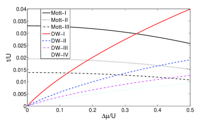
Figure 4: (Color online) Maxima of Mott-$n$ and DW-$n$ lobes as a function of $\Delta\mu$ for a 3$d$ cubic superlattice.

V Comparison with decoupled Mean-Field Theory

In order to treat a superlattice system with the decoupled mean-field theory, the operators $\hat{a}^{{\dagger}}_{i}$($\hat{a}_{i}$) are decomposed into the mean fields $\psi_{i}^{*}$ ($\psi_{i}$), which are identified with the order parameters, and the remaining operators $\delta\hat{a}^{{\dagger}}_{i}$($\delta\hat{a}_{i}$), which describe the quantum fluctuations around the mean fields. Then, after neglecting second order terms of the quantum fluctuations and assuming due to homogeneity that the order parameters are equal in the same subsystem, the Bose-Hubbard Hamiltonian (1) decouples into a mean-field Hamiltonian on two subsystems vezzani ; hou ; shuchen ; das1 :

$$\hat{H}_{\rm MF} = \hat{H}_{0}+tz\Big{(}\psi_{A}^{*}\psi_{B}+\psi_{B}^{*}\psi_{A}$$ (39)

$$-\hat{a}_{A}^{\dagger}\psi_{B}-\hat{a}^{\dagger}_{B}\psi_{A}-\hat{a}_{A}\psi_{B}^{*}-\hat{a}_{B}\psi_{A}^{*}\Big{)}\,,$$

with $\hat{H}_{0}$ from (52). Because the order parameters are tiny near the boundary of the second-order phase transition, the corresponding free energy can be Taylor expanded with respect to both order parameters

$$F_{\rm MF} = f_{0}+f_{2A}\left|\psi_{A}\right|^{2}+f_{2B}\left|\psi_{B}\right|^{2}+f_{2AB}\psi_{A}\psi_{B}^{*}$$ (40)

$$+f_{2BA}\psi_{B}\psi_{A}^{*}+...\,,$$

where the leading term $f_{0}$ is equal to the leading term $F_{0}(t)$ of GEPLT at $t=0$. Thus, from the previous analysis on $F_{0}(t=0)=N_{s}E^{(0)}\left(n_{A},n_{B}\right)$ with Eq. (32), we obtain the restrictions (37) and (38) for the chemical potential in the Mott insulator and density wave phases, respectively. As we only consider the system at zero temperature, the free energy is equivalent to the ground-state energy, which can be calculated perturbatively in the occupation number representation. With this we get the second-order coefficients

$$f_{2A} =t^{2}z^{2}\left[\frac{n_{B}}{U\left(n_{B}-1\right)-\mu}+\frac{n_{B}+1}{\mu-Un_{B}}\right]\,,$$

$$f_{2B} =t^{2}z^{2}\left[\frac{n_{A}}{U\left(n_{A}-1\right)-\mu-\Delta\mu}+\frac{n_{A}+1}{\mu+\Delta\mu-Un_{A}}\right]\,.$$

With the conditions (37) and (38) we find for both second-order derivatives the inequalities

$$\left.\frac{\partial^{2}F_{\rm MF}}{\partial\psi_{A}\partial\psi_{A}^{*}}\right|_{\psi_{A},\psi_{B}=0} = f_{2A}<0\,,$$

$$\left.\frac{\partial^{2}F_{\rm MF}}{\partial\psi_{B}\partial\psi_{B}^{*}}\right|_{\psi_{A},\psi_{B}=0} = f_{2B}<0\,.$$ (42)

This contradicts with the minimum condition which requires that both second-order derivatives are positive at $\psi_{A}=\psi_{B}=0$. We consider this to be a general problem of the multi-component decoupled mean-field theory, because it also happens in other systems such as Kagome and triangular systems. Note that it can be shown that a single-component mean-field theory does not have this minimum problem.

In order to proof that the GEPLT does not suffer from such a problem, we conclude at first from Eq. (29)

$$\left|\begin{array}[]{ccc}a_{2AA}&a_{2AB}\\ a_{2BA}&a_{2BB}\end{array}\right|=\frac{1}{\left|\begin{array}[]{ccc}-c_{2AA}&-c_{2AB}\\ -c_{2BA}&-c_{2BB}\end{array}\right|}$$ (43)

$$=\frac{1}{(\sqrt{c_{2AA}c_{2BB}}+c_{2AB})(\sqrt{c_{2AA}c_{2BB}}-c_{2AB})}\,.$$

Considering, for instance, the first-order result, we have in the Mott lobe $c_{2AB}^{(1)}=-tz\alpha_{2AA}^{(0)}\alpha_{2BB}^{(0)}<0$, $c_{2AA}^{(0)}=\alpha_{2AA}^{(0)}<0$, $c_{2BB}^{(0)}=\alpha_{2BB}^{(0)}<0$, so we get up to first order $\sqrt{c_{2AA}c_{2BB}}-c_{2AB}>0$. Considering $\sqrt{c_{2AA}c_{2BB}}+c_{2AB}=0$ is the phase boundary and $t$ is decreasing from the superfluid phase to the insulator phase, the denominator of Eq. (43) is positive in the insulator lobe which means

$$\left|\begin{array}[]{ccc}a_{2AA}&a_{2AB}\\ a_{2BA}&a_{2BB}\end{array}\right|>0$$ (46)

and

$$a_{2AA}=\frac{-c_{2BB}}{\left|\begin{array}[]{ccc}-c_{2AA}&-c_{2AB}\\ -c_{2BA}&-c_{2BB}\end{array}\right|}>0\,.$$ (49)

For the same reason, $a_{2BB}$ is also positive. Thus, the effective potential is really a local minimal at the zero point. Thus, in comparison with the decoupled mean-field approach GEPLT has the decisive advantage to be consistent for superlattice systems.

Another advantage of our method is its higher accuracy. In comparison with quantum Monte Carlo simulations, the error of the GEPLT is less than $3\%$ in second hopping order. And, according to our knowledge, such high accuracy is hard to reach by using other analytic methods. It can only be surpassed by higher hopping orders which could be evaluated via the process-chain approach of Refs. [Eckardt, ; Holthaus5, ; Holthaus6, ; Teichmann, ; Holthaus7, ].

However, the GEPLT also has its disadvantages. For the two-dimensional square superlattice system we can not get the full lobe of the phase boundary of the DW-I phase in the parameter range $\Delta\mu<0.35U$ in second hopping order, because the radicand of the square root in the phase boundary Eq. (31) becomes negative in second hopping order. We suspect that this is an artifact of truncating the hopping expansion at second order and expect that this could be corrected by obtaining higher hopping orders.

VI Conclusion and Outlook

In this paper, we extended the single-component effective potential Landau theory to the general case of a multi-component GEPLT method. In order to include several order parameters, we introduced the source vectors into the general multi-component Bose-Hubbard Hamiltonian. After performing the Legendre transformation of the free energy, we obtained a generalized effective potential, which can be determined in an expansion in hopping matrix elements. This method can be applied to the bosonic square and cubic superlattice systems yielding high accuracy results for the phase diagrams in second order hopping compared to QMC simulations. Apart from the Mott insulator phases, we also found competing DW phases with fractional filling factors which are induced by the translational symmetry breaking of the superlattice system. The dimensionality has a similar effect on the Mott insulator and the DW phases. Compared with the decoupled mean-field theory, the GEPLT has a higher accuracy and does not suffer from the local minimum problem. However, GEPLT also has a problem in calculating the whole quantum phase diagram for the DW-I phase which should be solved by considering higher order hopping corrections.

As the GEPLT turned out to be a general method for detecting second-order quantum phase transitions in a system with multi order parameters, we think it is also suitable for frustrated superlattice systems, such as the triangular and the Kagome lattice. Since the supersolid-solid phase transition for hard-core bosons is found to be of second order in the triangular lattice xuefeng , the GEPLT introduces a promising way to detect the quantum phase transition in both positive and negative hopping process regions. Furthermore, extending this work for finite temperatures and investigating the universal properties near the quantum phase boundary, are certainly worth for more detailed studies in the future.

Appendix A Strong-Coupling Peturbation Theory

The perturbative coefficients $\alpha_{2ll^{\prime}}^{(n)}$ follow at zero temperature from applying Rayleigh-Schrödinger perturbation theory using a suitable diagrammatic representation pelster2 . By denoting the creation (annihilation) operator with an arrow line pointing into (out of) the site, each perturbative contribution of $\alpha_{2ll^{\prime}}^{(n)}$ can be sketched as an arrow-line diagram which is composed of $n$ oriented internal lines connecting the vertices and two external arrow lines. The vertices in the diagram correspond to the respective lattice sites, oriented internal lines stand for the hopping process between sites, and the two external arrow lines are representing creation and annihilation operators, respectively. Table 1 presents all non-vanishing arrow-line diagrams as well as the associated multiplicities $\alpha_{2ll^{\prime}}^{(n)}$ up to the second hopping order.

Note that the arrow-line diagrams only depict the possible hopping processes. In order to determine each non-zero perturbative term $\alpha^{(n)}_{2ll^{\prime}}$, we also invoke a line-dot diagrammatic representation which has been worked out for a single component method in Ref. [pelster2, ]. To this end we consider the general situation that a Hamiltonian $\hat{H}$ decomposes into an unperturbed term $\hat{H}_{0}$ and two perturbation terms $\hat{V}$, $\hat{W}$, i.e.

$$\hat{H}=\hat{H}_{0}+\lambda\hat{V}+\delta\hat{W}\,,$$ (50)

where $\lambda$ and $\delta$ are small parameters. We then calculate the zero-temperature free energy by using perturbation theory. Each term is related to several line-dot diagrams which stem from the following rules:

• The dots labeled by $1$ and $2$ represent the perturbative terms $\hat{V}$ and $\hat{W}$, respectively.

• The internal lines connecting two adjacent dots are associated with the factor

  $$\sum_{m\neq n}\frac{1}{\left(E_{n}^{\left(0\right)}-E_{m}^{\left(0\right)}\right)^{p}}|\Psi_{m}^{\left(0\right)}\rangle\langle\Psi_{m}^{\left(0\right)}|\,,$$

  where the ground state of $\hat{H}_{0}$ is $|\Psi_{n}^{\left(0\right)}\rangle$ with the energy $E_{n}^{(0)}=\langle\Psi_{n}^{\left(0\right)}|\hat{H}_{0}|\Psi_{n}^{\left(0\right)}\rangle$ and $|\Psi_{m}^{\left(0\right)}\rangle$ represents an excited state with the energy $E_{m}^{(0)}$, whereas $p$ denotes the number of lines connecting two given consecutive dots.

• $\langle\Psi_{n}^{\left(0\right)}|$ and $|\Psi_{n}^{\left(0\right)}\rangle$ are denoted by left-external and right-external lines, respectively, so in the diagrammatic representation of $E_{n}^{\left(i\right)}$ there are some graphs which consist of $s$ disconnected parts. The weight of these graphs has to be multiplied by the sign $\left(-1\right)^{s-1}$.

$\alpha_{2AA}^{(0)}$		$\alpha_{2BB}^{(0)}$
$\alpha_{2AB}^{(1)}$	$z\includegraphics[width=62.59596pt]{2a.eps}$	$\alpha_{2BA}^{(1)}$	$z\includegraphics[width=62.59596pt]{2b.eps}$
$\alpha_{2AA}^{(2)}$	$z\includegraphics[width=71.13188pt,height=42.67912pt]{3a.eps}+z(z-1)\includegraphics[width=93.89418pt]{4a.eps}$
$\alpha_{2BB}^{(2)}$	$z\includegraphics[width=71.13188pt,height=42.67912pt]{3b.eps}+z(z-1)\includegraphics[width=93.89418pt]{4b.eps}$

Table 1: Diagrammatic arrow line expressions of the non-vanishing elements $\alpha_{2ll^{\prime}}^{(n)}$ including their multiplicities for a square and cubic superlattice up to second hopping order. The coordinate number $z$ is $2d$ for a $d$ dimensional hypercubic lattice.

With these rules, we obtain within the line-dot representation the perturbative expansion

$$E_{n}=E_{n}^{(0)}+\lambda\raisebox{-1.42271pt}{\hskip 1.42271pt\includegraphics[width=28.45274pt]{linedot1.eps}\hskip 1.42271pt}+\delta\raisebox{-1.42271pt}{ \hskip 1.42271pt\includegraphics[width=28.45274pt]{linedot2.eps}\hskip 1.42271pt}+\lambda\delta\left(\raisebox{-1.42271pt}{\hskip 1.42271pt\includegraphics[width=39.83368pt]{linedot3.eps}\hskip 1.42271pt}\right.$$

$$\left.+\raisebox{-1.42271pt}{\hskip 1.42271pt\includegraphics[width=39.83368pt]{linedot4.eps}\hskip 1.42271pt}\right)+\lambda^{2}\raisebox{-1.42271pt}{\hskip 1.42271pt\includegraphics[width=39.83368pt]{linedot5.eps}\hskip 1.42271pt}+\delta^{2}\raisebox{-1.42271pt}{\hskip 1.42271pt\includegraphics[width=39.83368pt]{linedot6.eps}\hskip 1.42271pt}$$ (51)

$$+\lambda^{2}\delta\left(\raisebox{-1.42271pt}{\includegraphics[width=51.21504pt]{linedot7.eps}}+\raisebox{-1.42271pt}{\includegraphics[width=51.21504pt]{linedot8.eps}}+\raisebox{-1.42271pt}{\includegraphics[width=51.21504pt]{linedot9.eps}}\right.$$

$$\left.+\raisebox{-14.22636pt}{\includegraphics[width=51.21504pt]{linedot10.eps}}+\raisebox{-14.22636pt}{\includegraphics[width=51.21504pt]{linedot11.eps}}+\raisebox{-14.22636pt}{\includegraphics[width=51.21504pt]{linedot12.eps}}\right)+\cdots\,.$$

In our concrete case of the square and cubic superlattice with the Hamiltonian in Eq. (1), the unperturbed Hamiltonian is given by

$$\hat{H}_{0} = \frac{U}{2}\hat{n}_{A}\left(\hat{n}_{A}-1\right)+\frac{U}{2}\hat{n}_{B}\left(\hat{n}_{B}-1\right)$$ (52)

$$-(\mu+\Delta\mu)\hat{n}_{A}-\mu\hat{n}_{B}\,,$$

yielding the unperturbed energies (32), whereas both the hopping and current terms are treated as a perturbation. Thus this leads to the arrow diagrams within the coefficient $\alpha_{2ll^{\prime}}^{(n)}$, which can now be represented in terms of respective line-dot diagrams. Note that each term $\alpha_{2ll^{\prime}}^{(n)}$ consists of exactly one creation operator (associated with $J_{i}$), one annihilation operator (associated with $J_{i}^{*}$), and $n$ hopping operators (associated with $t^{n}$). For each arrow-line diagram we have to draw all possible topologically different line-dot diagrams. The sum of all these line-dot diagrams then gives the corresponding result. For example, the equation

$$\raisebox{-2.84544pt}{\includegraphics[width=56.9055pt]{link.eps}}=\raisebox{-1.42271pt}{\includegraphics[width=42.67912pt]{linedot3.eps}}+\raisebox{-1.42271pt}{\includegraphics[width=42.67912pt]{linedot4.eps}}\,,$$ (53)

where $i$ inside the dot stands for a particular sublattice, expresses exemplary how to transfer an arrow-line diagram into its line-dot representation. Following these steps one obtains for the respective coefficients $\alpha_{2ll^{\prime}}^{(n)}$ the results (34)–(36), where the abbreviations (32), (33) are used.

References

- (1) M. Lewenstein, A. Sanpera, V. Ahufinger, B. Damski, A. S. De, and U. Sen, Adv. Phys. 56, 243 (2007).
- (2) I. Bloch, J. Dalibard, and W. Zwerger, Rev. Mod. Phys. 80, 885 (2008).
- (3) M. Lewenstein, A. Sanpera, and V. Ahufinger, Ultracold Atoms in Optical Lattices: Simulating Quantum Many-Body Systems (Oxford University Press, Oxford, 2012).
- (4) M. P. A. Fisher, P. B. Weichman, G. Grinstein, and D. S. Fisher, Phys. Rev. B 40, 546 (1989).
- (5) D. Jaksch, C. Bruder, J. I. Cirac, C. W. Gardiner, and P. Zoller, Phys. Rev. Lett. 81, 3108 (1998).
- (6) M. Greiner, O. Mandel, T. Esslinger, T. W. Hänsch, and I. Bloch, Nature 415, 39 (2002).
- (7) I. Bloch, J. Dalibard, and S. Nascimbène, Nature Phys. 8, 267 (2012).
- (8) P. T. Ernst, S. Gotze, J. S. Krauser, K. Pyka, D.-S. Luhmann, D. Pfannkuche, and K. Sengstock, Nature Phys. 6, 56 (2010).
- (9) U. Bissbort, S. Gotze, Y. Li, J. Heinze, J. S. Krauser, M. Weinberg, C. Becker, K. Sengstock, and W. Hofstetter, Phys. Rev. Lett. 106, 205303 (2011).
- (10) A. Lauer, D. Muth, and M. Fleischhauer, New J. Phys. 14, 095009 (2012).
- (11) P. Schauß, M. Cheneau, M. Endres, T. Fukuhara, S. Hild, A. Omran, T. Pohl, C. Gross, S. Kuhr, and I. Bloch, Nature 491, 87 (2012).
- (12) E. Altman, W. Hofstetter, E. Demler, and M. D Lukin, New J. Phys. 5, 113 (2003).
- (13) P. Soltan-Panahi, Dirk-Sören Lühmann, J. Struck, P. Windpassinger, and K. Sengstock, Nature Phys. 8, 71 (2012).
- (14) S. Piel, J. V. Porto, B. Laburthe Tolra, J. M. Obrecht, B. E. King, M. Subbotin, S. L. Rolston, and W. D. Phillips, Phys. Rev. A 67, 051603(R) (2003).
- (15) J. Sebby-Strabley, M. Anderlini, P. S. Jessen, and J. V. Porto, Phys. Rev. A 73, 033605 (2006).
- (16) S. Fölling, S. Trotzky, P. Cheinet, M. Feld, R. Saers, A. Widera, T.Muüller and I. Bloch, Nature 448, 1029 (2007).
- (17) P. Cheinet, S. Trotzky, M. Feld, U. Schnorrberger, M. Moreno-Cardoner, S. Fölling, and I. Bloch, Phys. Rev. Lett. 101, 090404 (2008).
- (18) G.-B. Jo, J. Guzman, C. K. Thomas, P. Hosur, A. Vishwanath, and D. M. Stamper-Kurn, Phys. Rev. Lett. 108, 045305 (2012).
- (19) J. M. Hou, Mod. Phys. Lett. B 23, 25 (2009).
- (20) K. D. Nelson, X. Li, and D. S. Weiss, Nature Phys. 3, 556 (2007).
- (21) T. Gericke, P. Würtz, D. Reitz, T. Langen, and H. Ott, Nature Phys. 4, 949 (2008).
- (22) P. Würtz, T. Langen, T. Gericke. A. Koglbauer, and H. Ott, Phys. Rev. Lett. 103, 080404 (2009).
- (23) N. Gemelke, X. Zhang, C.-L. Hung, and C. Chin, Nature 460, 995 (2009).
- (24) M. Karski, L. Förster, J. M. Choi, W. Alt, A. Widera, and D. Meschede, Phys. Rev. Lett. 102, 053001 (2009).
- (25) W. S. Bakr, J. I. Gillen, A. Pengh, S. Fölling, and M. Greiner, Nature 462, 74 (2009).
- (26) C. Weitenberg, M. Endres, J. F. Sherson, M. Cheneau, P. Schauß, T. Fukuhara, I. Bloch, and S. Kuhr, Nature 471, 319 (2011).
- (27) P. Buonsante and A. Vezzani, Phys. Rev. A 70, 033608 (2004).
- (28) S. Sachdev, Quantum phase transitions, Second Edition (Cambridge University Press, Cambridge, 2011).
- (29) V. G. Rousseau, D. P. Arovas, M. Rigol, F. Hebert, G. G. Batrouni, and R. T. Scalettar, Phys. Rev. B 73, 174516 (2006).
- (30) G. Roux, T. Barthel, I. P. McCulloch, C. Kollath, U. Schollwöck, and T. Giamarchi, Phys. Rev. A 78, 023628 (2008).
- (31) A. Dhar, T. Mishra, R. V. Pai, and B. P. Das, Phys. Rev. A 83, 053621 (2011).
- (32) B.-L. Chen, S.-P. Kou, Y. Zhang, and S. Chen, Phys. Rev. A 81, 053608 (2010).
- (33) A. Dhar, M. Singh, R. V. Pai, and B. P. Das, Phys. Rev. A 84, 033631 (2011).
- (34) T. McIntosh, P. Pisarski, R. J. Gooding, and E. Zaremba, Phys. Rev. A 86, 013623 (2012).
- (35) P. Pisarski, R. M. Jones and R. J. Gooding, Phys. Rev. A 83, 053608(2011).
- (36) D. Muth, A. Mering, and M. Fleischhauer, Phys. Rev. A 77, 043618(2008)
- (37) P. Buonsante, V. Penna and A. Vezzani, Laser Phys. 15, 361 (2005)
- (38) P. Buonsante and A. Vezzani, Phys. Rev. A 72, 013614(2005).
- (39) P. Buonsante, V. Penna, and A. Vezzani, Phys. Rev. A 72, 031602(R)(2005).
- (40) For a recent example see X.-F. Zhang, Q. Sun, Y.-C. Wen, W.-M. Liu, S. Eggert, and A.-C. Ji, Phys. Rev. Lett. 110, 090402 (2013).
- (41) A. Hoffmann and A. Pelster, Phys. Rev. A 79, 053623 (2009).
- (42) F. E. A. dos Santos and A. Pelster, Phys. Rev. A 79, 013614 (2009).
- (43) B. Bradlyn, F. E. A. dos Santos, and A. Pelster, Phys. Rev. A 79, 013615 (2009).
- (44) T. D. Graß, F. E. A. dos Santos, and A. Pelster, Phys. Rev. A 84, 013613 (2011).
- (45) L. zin, J. Zhang, and Y. Jiang, Phys. Rev. A 85, 023619 (2012).
- (46) M. Ohliger and A. Pelster, World J. Cond. Matt. Phys. 3, 125 (2013).
- (47) A. Eckardt, Phys. Rev. B 79, 195131 (2009).
- (48) N. Teichmann, D. Hinrichs, M. Holthaus, and A. Eckardt, Phys. Rev. B 79, 100503 (2009).
- (49) N. Teichmann, D. Hinrichs, M. Holthaus, and A. Eckardt, Phys. Rev. B 79, 224515 (2009).
- (50) N. Teichmann and D. Hinrichs, Europ. Phys. J. B 71, 129 (2009).
- (51) N. Teichmann, D. Hinrichs, and M. Holthaus, Europ. Phys. Lett. 91, 10004 (2010).
- (52) B. Capogrosso-Sansone, N. V. Prokof’ev, and B. V. Svistunov, Phys. Rev. B 75, 134302 (2007).
- (53) B. Capogrosso-Sansone, S. G. Söyler, N. V. Prokof’ev, and B. V. Svistunov, Phys. Rev. A 77, 015602 (2008).
- (54) D. Hinrichs, A. Pelster, and M. Holthaus, Appl. Phys. B. (in press), DOI 10.1007/s00340-013-5419-0
- (55) D. Hinrichs, M. Holthaus, and A. Pelster, in preparation
- (56) J. Zinn-Justin, Quantum Field Theory and Critical Phenomena, Fourth Edition (Oxford University Press, Oxford, 2002).
- (57) H. Kleinert and V. Schulte-Frohlinde, Critical properties of Theories (World Scientific, Singapore, 2001).
- (58) L. Fallani, J. E. Lye, V. Guarrera, C. Fort, and M. Inguscio, Phys. Rev. Lett. 98, 130404 (2007).
- (59) S.-L. Zhu, Z.-D. Wang, Y.-H. Chan, and L.-M. Duan, Phys. Rev. Lett. 110, 075303 (2013).
- (60) F. Grusdt, M. Hoening, and M. Fleischhauer, eprint: arXiv:1301.7242.
- (61) A. W. Sandvik, Phys. Rev. B 59, R14157 (1999).
- (62) O. F. Syljuåsen and A. W. Sandvik, Phys. Rev. E 66, 046701 (2002).
- (63) H. M. Guo, Y. C. Wen and S. P. Feng, Phys. Rev. A 79, 035401 (2009).
- (64) Our numerical phase diagram in 2d coincides with the unpublished numerical work of Xiaojuan Li and Yu-Chuan Wen.
- (65) X.-F. Zhang, Y.-C. Wen, and S. Eggert, Phys. Rev. B 82, 220501(R) (2010).
- (66) X.-F. Zhang, R. Dillenschneider, Y. Yu, and S. Eggert, Phys. Rev. B 84, 174515 (2011).