MITP/13-10
PSI-PR-13-18
April 8, 2013
Approximate NNLO Predictions for the Stop-Pair Production Cross Section at the LHC
Alessandro Broggioa,b, Andrea Ferrogliac, Matthias Neuberta,
Leonardo Vernazzaa,d and Li Lin Yange,f,g
aPRISMA Cluster of Excellence & Mainz Institut for Theoretical Physics
Johannes Gutenberg University, D-55099 Mainz, Germany
bPaul Scherrer Institute
CH-5232 Villigen, Switzerland
cNew York City College of Technology
300 Jay Street,
Brooklyn, NY 11201, USA
dDipartimento di Fisica, Università di Torino & INFN, Sezione di Torino
Via P. Giuria 1, I-10125 Torino, Italy
eInstitute for Theoretical Physics
University of Zurich,
CH-8057 Zurich, Switzerland
fSchool of Physics and State Key Laboratory of Nuclear Physics and Technology
Peking University, 100871 Beijing, China
gCenter for High Energy Physics, Peking University, Beijing 100871, China
If the minimal supersymmetric standard model at scales of around TeV is realized in nature, the total top-squark pair production cross section should be measurable at the CERN Large Hadron Collider. In this work we present precise predictions for this observable, which are based upon approximate NNLO formulas obtained using soft-collinear effective theory methods.
1 Introduction
One of the main goals of the physics program at the Large Hadron Collider (LHC) is to investigate the existence of supersymmetric partners of the fundamental particles with masses in the TeV range. Within the context of the minimal supersymmetric standard model (MSSM) with R-parity conservation, supersymmetric particles are produced in pairs. At hadron colliders, the supersymmetric particles which are expected to be most abundantly produced are the ones which carry color charge: squarks and gluinos. Since supersymmetry is broken, the mass spectrum of squarks and gluinos plays a crucial part in determining which among the colored supersymmetric partners is experimentally accessible. Within the context of unified supersymmetric theories, the scalar and gaugino masses are evolved from a common high scale down to the energy scale of electroweak symmetry breaking. As a consequence of large Yukawa and soft couplings entering the evolution of the mass parameters, the third generation of squarks can have very different masses compared to the first two generations of squarks. In particular, under the assumption of “natural supersymmetry” [1], top-squarks are expected to be relatively light in order to reproduce the correct energy scale of electroweak symmetry breaking. Therefore, the lightest of the two supersymmetric partners of the top quark is usually expected to be the lightest squark in the mass spectrum. Precise theoretical predictions of the stop pair production cross section are instrumental in setting a lower bound on the lightest stop mass. Moreover, if top squarks will be discovered, accurate predictions of the cross section for stop pair production can be employed to determine the masses and other properties of these particles. For these reasons, the study of the radiative corrections to the production of stop pairs has already a quite long history. The calculation of the next-to-leading order (NLO) corrections to the cross section for stop pair production within the context of supersymmetric quantum chromodynamics (SUSY-QCD) was completed 15 years ago [2]. As expected, it was found that the NLO corrections significantly decrease the renormalization- and factorization-scale dependences of the prediction when compared to the leading order (LO) calculation. Furthermore, NLO SUSY-QCD corrections increase the value of the cross section if the renormalization and factorization scales are chosen close to the value of the stop mass. The NLO SUSY-QCD corrections are implemented in the computer programs Prospino and Prospino2 [3]. The electroweak corrections to stop pair production were studied in [4, 5]. While these corrections have a quite sizable effect on the tails of the invariant-mass and transverse-momentum distributions, they only have a moderate impact on the total cross section. The emission of soft gluons accounts for a significant portion of the NLO SUSY-QCD corrections [6], which are large. For this reason, the resummation of the next-to-leading logarithmic (NLL) corrections was carried out in [7]. It was found that these corrections increase the cross section at the LHC by up to of its NLO value, while they further decrease the scale dependence of the prediction. In [8, 9, 10] next-to-next-to-leading order (NNLO) threshold corrections and Coulomb corrections were derived by means of resummation techniques. In these studies, the resummation is carried out in Mellin moment space.
In the last few years, a formalism based on soft-collinear effective theory (SCET), which allows one to resum soft-gluon corrections directly in momentum space, was developed [11, 12] and applied to QCD corrections for several processes of interest in collider phenomenology, such as Drell-Yan scattering [13], Higgs production [14, 15], direct photon production [16], and recently slepton pair production [17]. A similar approach was developed independently in [18], where methods of SCET and non-relativistic QCD were used to resum simultaneously the effects of soft and Coulomb gluons. This method was applied to squark and gluino pair production [18, 19], where soft and Coulomb-gluon contributions were resummed at NLL order, and to top-quark pair production [20], where resummation up to next-to-next-to-leading logarithmic (NNLL) order was implemented. The soft-gluon corrections to the top-quark pair production cross section at the Tevatron and the LHC were also studied in [21, 22], within the framework developed in [11, 12]. By employing this formalism, it was possible to resum soft-gluon emission corrections up to NNLL accuracy, as well as to derive approximate NNLO formulas for the total production cross section, the pair invariant-mass distribution, the top-quark transverse-momentum spectrum, and the top-quark rapidity distribution.
In fixed-order perturbation theory, differential partonic cross sections involve both singular distributions and regular terms. The singular distributions are functions of a “soft parameter”, whose precise definition depends on the kinematics. In [21, 13], where pair-invariant mass (PIM) kinematics was employed, the relevant soft parameter is , where is the partonic center of mass energy, , and is the pair invariant mass of the energetic particles produced. In this case, the soft (or partonic-threshold) region corresponds to the limit . In [22], where one-particle inclusive (1PI) kinematics was employed, the relevant soft parameter is , which is obtained by subtracting the heavy-particle mass squared from the invariant mass of the objects recoiling against the observed heavy particle. In this case, the soft gluon emission region is identified by taking the limit . Detailed studies of Drell-Yan and top pair production processes showed that, after the convolution of the hard-scattering kernels with the parton luminosities, the terms which are singular in the partonic-threshold limit provide the numerically dominant contributions to the hadronic cross sections. In these processes, the singular terms typically account for more than 90% of the total NLO corrections. Furthermore, the dominance of the partonic-threshold regions in the calculation of the cross sections arises dynamically, since it is due to the strong fall-off of the parton luminosities outside the threshold region. This phenomenon is called “dynamical threshold enhancement” [13].
In the partonic-threshold region, the partonic cross sections factorize into the product of hard functions, which contain the virtual corrections to the cross section, and soft functions, which account for the effects of soft gluon emissions. The singular (plus) distributions in the partonic cross section can be obtained by solving the renormalization group equations (RGEs) satisfied by the hard and soft functions. The corresponding anomalous dimensions are known up to NNLO [23, 24]. The information extracted from the RGE and the knowledge of the hard and soft functions at NLO allows us to obtain approximate formulas including all of the singular terms up to NNLO. These approximate NNLO formulas can then be matched with exact NLO calculations in order to obtain precise theoretical predictions for the observables of interest.
Within this context, the production of top-squark pairs in the soft-gluon emission limit can be studied in analogy to the production of top-quark pairs. The hard and soft functions are matrices in color space. The soft functions in the stop-quark and top-quark production processes are identical; they were evaluated in [21, 22] up to NLO. In contrast, the hard functions for the stop-pair production process are so far unknown and must be computed with NLO accuracy. It is important to observe that the only SUSY parameter which appears in the soft functions is the mass of the produced stop quark, while all of the other SUSY parameters appear exclusively in the hard functions. In this work, we carry out the calculation of the hard functions for top-squark pair production up to NLO. By combining the NLO hard functions with the NLO soft functions and with the anomalous dimensions entering the RGEs satisfied by the various terms in the factorized cross section, it is possible to resum soft-gluon emission corrections up to NNLL order. Here we limit ourselves to re-expand the resummed formulas in order to obtain approximate NNLO formulas for the pair invariant-mass spectrum and the stop transverse-momentum and rapidity distributions. Although our formulas enable us to obtain predictions for these differential distributions, we focus our attention on the total top-squark production cross section, which is the observable of most immediate interest in the top squark searches. In fact, by integrating the approximate NNLO formulas for the differential distributions over the complete phase-space, we obtain predictions for the total top-squark pair production cross section at the LHC, and we comment on the phenomenological impact of the NNLO corrections arising from soft emissions. In a future work, we will evaluate the resummed stop pair production cross section and discuss the phenomenological impact of soft gluon resummation at NNLL accuracy. It must be remarked that the resummation at NNLL accuracy, in Mellin space, is already available for the production of other SUSY particles; the production of squark pairs was carried out in [25], while the production of gluino pairs was studied at this level of accuracy in [26]. Furthermore the NLO hard matching coefficients for squark and gluino hadroproduction, an important ingredient for NNLL studies, were evaluated very recently [27].
The paper is organized as follows: In Section 2 we introduce our notation and conventions, which are very similar to the ones employed in [21, 22]. Furthermore, we describe the factorization of the stop pair production cross section in the soft limit, both in PIM kinematics and in 1PI kinematics. In Section 3, we discuss the calculation of the soft and hard functions up to NLO. In Section 4, we discuss the structure of the hard scattering kernels and we present approximate NNLO formulas for the stop pair production process. Predictions for the total top-squark pair production cross section at the LHC can be found in Section 5, together with an analysis of the phenomenological impact of the approximate NNLO corrections on this observable. We conclude Section 5 by comparing our results with the NLO+NLL results of and [7] and [19], which are obtained by means of techniques and kinematic schemes different from the ones that we employ in this work. Finally, we collect our conclusions in Section 6.
2 Notation
In this paper we study the process
| (1) |
where and indicate the incoming protons in the case of a proton-proton collider as the LHC, while is an inclusive hadronic final state. In the rest of the paper, we treat the top squarks as on-shell particles and neglect their decay. The terms neglected in this approximation are of order . At the lowest order in perturbation theory, two partonic channels contribute to the process in Eq. (1):
| (2) |
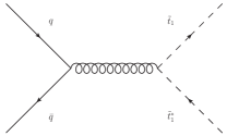
where the momenta of the incoming partons are related to the momenta of the incoming hadrons by (). The diagrams contributing to the two production channels at lowest order in QCD are shown in Figure 1.
 |
 |
The relevant invariants for the hadronic scattering are
| (3) |
In order to describe the partonic scattering, we employ the invariants
| (4) |
In Born approximation , and consequently and .
It is well known that the kinematics of the process allows one to define different threshold regions. Here we consider two different cases: PIM kinematics, in which the threshold region is defined by the limit , and 1PI kinematics, in which the threshold region is approached by taking the limit . Both regions were employed in the study of the top-quark pair production cross section and differential distributions [28, 29, 21, 22]. In particular, by working in PIM kinematics one can calculate the pair invariant-mass distribution, while by working in 1PI kinematics one can evaluate the stop transverse-momentum and rapidity distributions. It should be emphasized that in the PIM and 1PI threshold regions the top squarks are not forced to be nearly at rest, as in case of the threshold region defined by the limit , which is often employed in the calculation of soft-gluon corrections to the total cross section [7, 18, 19]. In the rest of the paper, we refer to the limit as the production threshold region.
Our goal is to employ both PIM and 1PI kinematics to obtain approximate NNLO formulas for the total top-squark pair production cross section. Both approaches include the numerically large contributions arising from the emission of soft gluons. Differences between them, and with the production threshold calculations, arise from the way in which different sets of power-suppressed corrections are treated.
2.1 PIM kinematics
We focus first on the case of PIM kinematics. It is convenient to introduce the quantities
| (5) |
Consequently, the PIM threshold limit corresponds to the limit . According to the QCD factorization theorem [30], the differential cross section in and (the scattering angle of the top squark with respect to the beam axis in the partonic rest frame) is given by
| (6) |
where is the factorization scale, and the sum runs over the incoming partons. In the following we drop the subscript PIM (and the corresponding subscript 1PI) whenever there is no ambiguity about the kinematic scheme employed, or when a formula applies to both schemes. The parton luminosities are defined as the convolutions of the non-perturbative parton distribution functions (PDF) for the incoming partons and :
| (7) |
The functions in Eq. (6) are the hard-scattering kernels, which are related to the partonic cross sections and can be calculated in perturbation theory. In order not to clutter the notation, we do not indicate explicitly the fact that the hard-scattering kernels depend on the top-squark masses and , the mass of the first two generations of squarks and of the sbottoms (which we assume to be all degenerate), the top-quark mass , the gluino mass , and the - mixing angle . The expansion of the functions in powers of has the generic form
| (8) |
Only the quark annihilation and gluon fusion channels contribute to at lowest order in perturbation theory; in particular
| (9) |
where , and the Mandelstam invariants and can be written in terms of and as
| (10) |
In order to calculate higher-order corrections to and one needs to consider virtual and real-emission corrections to the Born approximation. Starting at order , new production channels, such as , open up. When working in the threshold limit , the calculations are simplified by the fact that there is no phase-space available for the emission of additional (hard) partons in the final state. Consequently, both the hard-gluon emission and the additional production channels are suppressed by powers of and can be safely neglected while deriving results within the partonic-threshold limit. By neglecting power-suppressed terms in the integrand, Eq. (6) can be rewritten as
| (11) |
In Eq. (11) the quark channel luminosities and are understood to be summed over all light quark flavors. The two terms in the second line of Eq. (11) differ in the fact that in the first term the quark (antiquark) comes from the hadron () in Eq. (1), while in the second term the quark (antiquark) comes from the hadron (), respectively. The total cross section can be obtained by integrating over in the range and over in the range .
In the soft-gluon emission limit , the hard-scattering kernels factor into a product of hard and soft functions:
| (12) |
Here and in what follows we employ boldface fonts to indicate matrices in color space, such as the hard functions and the soft functions . For simplicity we drop the the top mass and the SUSY parameters from the list of arguments of the hard functions , as well as the stop mass from the arguments of the soft functions . Throughout this paper, we work in the -channel singlet-octet basis
| (13) |
where represent the color index of the particle with momentum . We view these structures as basis vectors in the space of color-singlet amplitudes. Inner products in this space are defined through a summation over color indices as
| (14) |
This inner product is proportional but not equal to , so the basis vectors are orthogonal but not orthonormal.
A factorization formula analogous to Eq. (12) for the top-quark pair production was derived employing SCET and heavy-quark effective theory in [21]. A completely analogous procedure can be followed in order to derive Eq. (12), which is valid in the case of top-squark pair production.
The hard functions are obtained from the virtual corrections and are ordinary functions of their arguments. The soft functions arise from the real emission of soft gluons and contain distributions which are singular in the limit. Contributions of order to the soft functions include terms proportional to the plus distributions
| (15) |
as well as terms proportional to . In particular, the NLO and NNLO hard-scattering kernels in Eq. (8) have the structure
| (16) |
The functions , , and depend also on , , and on the heavy-particles masses. The coefficients , , and can in principle be obtained from results present in the literature. One of the main results of this paper is the calculation of the coefficients (with ) both in the quark annihilation and gluon fusion channels. We can also evaluate all of the scale-dependent terms in in both channels, but due to the ambiguity on the choice of the normalization scale in the argument of these logarithms we drop part of these terms in the numerical implementation of our formulas. We will return to this issue below.
2.2 1PI kinematics
The 1PI kinematics approach allows one to describe observables in which a single particle, rather than a pair, is considered. One can then write the top-squark rapidity () and transverse-momentum () distribution as
| (17) |
once again we will drop the subscript 1PI in most of our equations below. The expansion of the 1PI hard-scattering kernels in powers of has the same structure shown in Eq. (8) for the PIM case. Obviously, also in this case only the and channels give non-vanishing contributions at lowest order in . The hadronic Mandelstam variables and are related to the stop rapidity and transverse momentum through the relations
| (18) |
where . Therefore, the variables , , which are arguments of the 1PI hard functions can be expressed in terms of , . The lower integration limits in Eq. (17) are
| (19) |
In order to obtain the total cross section, it is necessary to integrate the double-differential distribution with respect to the top-squark rapidity and transverse momentum over the range
| (20) |
In the case of 1PI kinematics, the hard-scattering kernels in the soft-emission limit factor into a product of hard and soft functions, in analogy with Eq. (12):
| (21) |
As emphasized in [22], the Mandelstam invariants , can differ from , by power corrections proportional to . For example, explicit results for the hard and soft functions can be rewritten by employing either the relation or . The difference between the two choices is due to terms suppressed by positive powers of . A detailed description of the way in which we deal with this ambiguity can be found in Section 4 of [22].
As in the case of PIM kinematics, the hard and soft function are matrices in color space originating from virtual and soft-emission corrections, respectively. The 1PI hard functions are identical to the ones encountered in the case of PIM kinematics, provided that the variables , and are written in terms of and . The soft functions are different in the PIM and 1PI schemes, but in both cases they are identical to the ones employed in the calculation of the top-quark pair production cross sections in [21, 22].
The 1PI soft functions at order depend on the associated plus distributions
| (22) |
It follows that
| (23) |
where is a smooth test function. At NLO and NNLO, the hard-scattering kernel in 1PI kinematics have the structure
| (24) |
As in the PIM case, the NLO coefficients , , and can be in principle obtained from the literature. In this work we are able to derive exact expressions for the NNLO coefficients (with ) and the scale-dependent terms in the coefficients .
3 The hard and soft functions at NLO
In this section we describe the calculation of the soft and hard matrices up to NLO in perturbation theory.
3.1 Hard functions
As it was shown in detail in [21], the hard functions are defined in terms of the products of Wilson coefficients with their complex conjugates. In order to obtain the Wilson coefficients, one matches renormalized Green’s functions in SUSY-QCD with those in SCET. The matching procedure can be carried out by choosing arbitrary external states and infrared (IR) regulators. The simplest and most common procedure consists in employing on-shell states for the partonic processes and in using dimensional regularization to regulate both IR and ultraviolet (UV) divergences. With this choice, the SCET loop diagrams vanish because they are scaleless. Consequently, the effective theory matrix elements are equal to their tree-level expressions multiplied by a UV renormalization matrix . The SUSY-QCD matrix elements are instead the virtual corrections to the scattering amplitudes of the partonic processes .
Rather than implementing the matching condition for the Wilson coefficients, we directly move to the calculation of the the matrix elements of the hard functions projected onto a certain basis of color structures. These matrix elements, and not the Wilson coefficients, are needed in order to obtain the approximate NNLO formulas which represent the main result of the present work. Throughout this paper, we use the -channel singlet-octet basis defined in Eq. (13). In order to calculate the hard-function matrix elements, we use the fact that the renormalized hard functions can be directly obtained from the corresponding (squared) on-shell QCD scattering amplitudes. The infrared poles can be removed from the QCD amplitudes by employing the prescription of [31, 32]
| (25) |
where the indices are not summed over. Here are the dimensionally regularized (and UV renormalized) scattering amplitudes, whose IR poles are removed by the factors . The resulting finite amplitudes are expressed in terms of with active flavors. The explicit form of the matrices can be obtained by employing the results derived in [33, 23, 24].
The perturbative expansion of the renormalized hard functions is defined as
| (26) |
where in the quark annihilation channel and in the gluon fusion channel. The desired matrix elements can then be written in terms of the renormalized QCD amplitudes and the color basis vectors as
| (27) |
The leading-order result for the channel follows from a simple calculation. In matrix notation, it reads
| (28) |
while that for the channel is
| (29) |
In order to calculate the NLO hard matrices , one needs to evaluate the one-loop corrections to the partonic scattering amplitudes, by keeping the various color components separate. Although results for the corresponding one-loop diagrams interfered with the Born-level amplitudes are well known [2], their decomposition into the color basis is not available in the literature, and we therefore had to calculate it from scratch. For this purpose, we have used in-house routines written in the computer algebra system FORM [34] in combination with Reduze [35, 36]. The results of the calculation are expressed in terms of Passarino-Veltman functions [37]. After UV renormalization, we have derived analytic expressions for the IR poles, and we have evaluated the finite parts of the amplitudes numerically by employing the programs described in [38, 39, 40]. We have checked our results in several ways. First, by applying the IR renormalization factors of Eq. (25), we find that the IR poles cancel exactly. Second, we have checked that by multiplying the one-loop hard functions with the corresponding tree-level soft functions and by subsequently taking the trace of the resulting color-space matrices, we reproduce the numerical results for the NLO virtual corrections which can be extracted from the code Prospino [3].
The output of our FORM codes are too long to be presented here in explicit form. The explicit expressions for the NLO hard functions are coded in a Mathematica and a Fortran program which are included in the arXiv version of this work. In particular, these programs allow one to evaluate numerically the LO and NLO hard functions for an arbitrary choice of the input parameters.
3.2 Soft functions
The soft functions are vacuum expectation values of soft Wilson-loop operators. These functions are not sensitive to the spin of the particles involved, but they depend on the color structure of the underlying partonic subprocesses. Consequently, the soft functions needed for the calculation of the top-squark pair-production cross section are precisely the same functions employed in the calculation of the cross section for top-quark pair production. The calculation of the PIM soft functions at NLO was described in detail in [21], while the analogous calculation of the 1PI soft functions was carried out in [22]. For the convenience of the reader, the explicit results for the soft functions obtained in those two papers are collected in Appendix A.
4 Structure of the hard scattering kernels
4.1 Preliminaries
Since the soft functions in (12) and (21) depend on plus distributions, it is more convenient to work with the Laplace-transformed functions
| (30) |
in PIM and similarly in the case of 1PI kinematics. It was shown in [12, 11, 13, 29] that the leading singular terms in the hard-scattering kernels can be generated by replacing the Laplace variable with a derivative with respect to an auxiliary variable , which is later set to 0. To this end, one defines Laplace-transformed hard-scattering kernels in PIM kinematics as
| (31) |
For 1PI kinematics one replaces the arguments and with , , and . The hard-scattering kernel in momentum space can then be recovered through the relations [29, 21, 22]
| (32) |
In order to evaluate the above formulas, one needs to employ analytic continuation to regulate the divergences in or , to take the derivatives with respect to , and finally to take the limit . It is possible to show that the result of this procedure can equivalently be obtained by implementing a series of replacement rules on the functions considered as polynomials in a new variable . In PIM kinematics, one must substitute
| (33) |
where , and the plus distributions have been defined in Eq. (15). In 1PI kinematics, one must substitute instead
| (34) |
where , , , and the associated plus distributions have been defined in Eq. (22).
Since the hard and soft functions are known up to NLO, is easy to determine the NLO coefficient in the expansion of in powers of :
| (35) |
It is important to observe that the trace of the product of the LO hard function and NLO soft function contains the dependence of on , and therefore it gives rise to the plus distributions. In order to obtain the complete coefficient one needs to know the hard and soft functions up to NNLO:
| (36) |
The NLO hard and soft functions in this equation are know exactly. As explained in detail in [21, 22], the scale-dependent part of the NNLO hard function and the dependent part of the NNLO soft function can be reconstructed by exploiting the information coming from the RGE satisfied by these functions. To this end, one only needs the one-loop hard and soft matrices calculated in Section 3 and in [21, 22], respectively, as well as the relevant two- and three-loop anomalous dimensions computed in [23, 24, 41, 42]. After this information on the NNLO hard and soft function has been extracted, one can evaluate the coefficients with in Eq. (36), as well as the scale-dependent part of .
4.2 Approximate NNLO formulas
| GeV | |||
|---|---|---|---|
| GeV | |||
| GeV | GeV | ||
| GeV | |||
| GeV |
By employing the results described in the previous sections, we are able to obtain approximate NNLO formulas for the hard-scattering kernels in Eqs. (12) and (21). These formulas include the exact expressions of the coefficients multiplying the plus distributions up to NNLO, both in PIM and in 1PI kinematics. The complete results for these coefficients, written in terms of Passarino-Veltman functions, are too lengthy to be reported here. The values of the coefficients multiplying the various plus distributions and delta functions for arbitrary values of the input parameters can be extracted from the Mathematica code mentioned above, which we include in the arXiv submission of this work.111The Mathematica file requires the use of LoopTools [38]. As a reference for the reader, we present here the hard scattering kernels evaluated by setting the input parameters at the values listed in Table 1. The SUSY spectrum which we chose corresponds to the benchmark point 40.2.5 in [43]; we employ this benchmark point for the remainder of this paper. By defining (), in the quark annihilation channel with PIM kinematics one finds
| (37) |
where the ellipses indicate terms which are subleading (and finite) in the limit. In the gluon fusion channel, we find instead
| (38) |
In order to completely determine the coefficients multiplying the delta functions in the NNLO hard-scattering kernels, one would need to know the complete NNLO hard and soft matrices. Since those matrices are at present not fully known at NNLO, we are only able to determine the scale-dependent terms in the delta-function coefficients, because those terms are governed by RGEs. However, since the scale-independent parts are unknown, the coefficients of the delta function at NNLO depend on an arbitrary second scale chosen to normalize the scale-dependent logarithms. In fact, for any renormalization scale and reference scale , one can always rewrite
| (39) |
where the second term in the r.h.s. can be reabsorbed in the unknown -independent piece. In Eq. (37) and Eq. (38), we chose the reference scale equal to the pair invariant mass . Furthermore, in Eq. (37) and Eq. (38), we decided to separate out the contributions to the delta-function coefficients coming from the NNLO hard functions. In particular, in the round brackets multiplying the delta functions, the second number represents the contributions of the scale-dependent terms in . In our numerical analysis in Section 5, we decided to drop the contributions to the NNLO delta-function coefficients arising from the two-loop hard functions. As was observed in [22], this choice is motivated by the fact that by including these -dependent terms one might induce an artificial reduction of the scale dependence, which can lead to an underestimated scale uncertainty.
Similarly, in 1PI kinematics we find for the quark annihilation channel
| (40) |
while for the gluon fusion channel we obtain
| (41) |
In this context, the ellipses indicate subleading terms in the limit. Also, in Eqs. (40) and (41), as in the PIM case, the scale-dependent terms are normalized to the scale , which is equal to when . As in the PIM case, also in Eqs. (40) and (41) the second number in the round brackets multiplying the delta functions in the NNLO kernels represents the contribution of the scale-dependent terms arising from the NNLO hard functions.
5 Total cross section
In this section we present a brief numerical study of the top-squark total pair production cross section at approximate NNLO accuracy. We stress that our approximate NNLO predictions include the full NLO corrections, as well as the part of the NNLO corrections arising from soft gluon emission, obtained by means of the procedure outlined in the previous sections.
Following what was done in the study of the top-quark pair production total cross section, we employ and kinematic schemes described in [44]. These schemes also include, on top of contributions which are singular in the soft limit, NNLO terms which are regular in the () or () limits, and which naturally arise from the SCET formalism. These terms, which are part of the functions in Eqs. (2.1) and (2.2), do not represent the complete contribution to the NNLO cross section which is regular in the soft limit, since this quantity can only be obtained with a full calculation of this observable at NNLO accuracy. However, as shown in [21, 22], the regular terms appearing in the and kinematic approaches arise from the exact definition of the soft-gluon emission energy, and they improve the agreement between exact and approximate formulas at NLO.
Unless otherwise stated, we present results which are obtained by averaging the ones obtained in the two kinematic schemes that we consider. In analogy with what was done in [44] for the top-quark pair production cross section, we adopt a conservative approach and consider the difference between the predictions in the two kinematic schemes as an estimate of the uncertainty associated with the use of approximate NNLO formulas. This is justified by the fact that the two schemes neglect different power-suppressed terms, which are formally subleading but which can nevertheless have a noticeable numerical impact on the total cross section. To account for this uncertainty, the scale variation of the total cross section is obtained by setting the renormalization and factorization scales equal to each other, , and by varying this single scale between . We then look at the difference between the largest and smallest values obtained. In summary, the central value and perturbative uncertainties for the combined results at approximate NNLO accuracy are determined by employing the definitions
| (42) |
where the subscripts 1PI and PIM indicate that the corresponding quantities are evaluated in and kinematics, respectively, including the full set of NLO corrections and the contribution of the NNLO terms present in the approximate formulas for that scheme.
As will be shown later, the total cross section is strongly dependent on the mass of the produced particle, . However, similarly to the slepton-pair production case [17], the dependence of the total cross section on other SUSY parameters is relatively small. In order to show that this is indeed the case, we fix the value of the stop mass equal to GeV, corresponding to the SUSY benchmark point 40.2.5 of [43] (which is defined in Table 1), and we provide predictions for the total cross section for three different sets of the remaining SUSY parameters. The first set of SUSY parameters coincides with the benchmark point 40.2.5 itself. The second set is defined by choosing GeV, GeV, GeV, . The values above are the double of the corresponding values of the benchmark point 40.2.5, and for this reason we label this second set of SUSY parameters as “double”. (The value of is kept fixed at GeV.) Similarly, the third set of SUSY parameters (which we refer to as “half”) is GeV, GeV, GeV, . The values of the total cross sections, with the relative perturbative uncertainty, for the three different SUSY parameters sets discussed above, can be found in Table 2. The table refers to a collider energy of TeV and the PDFs employed are from the MSTW2008 global fit [45, 46, 47]. We observe that the numerical values for the cross section are very close to each other, in spite of the fact that the input SUSY parameters are considerably different in the three sets. This is true both at NLO and at approximate NNLO accuracy.
| LHC TeV | MSTW2008 | |
|---|---|---|
| SUSY point | [GeV] | 1087.17 |
| 40.2.5 | [pb] | |
| “double” | [pb] | |
| “half” | [pb] | |
| 40.2.5 | [pb] | |
| “double” | [pb] | |
| “half” | [pb] | |
In all of the plots and tables discussed below, the SUSY parameters are set to the values corresponding to the benchmark point 40.2.5 in Table 1. This applies also to the lightest stop mass, with the exception of the figures in which we plot the cross section as a function of the stop mass or when a different choice of the stop mass is explicitly indicated.
All of the numbers and plots are obtained by means of an in-house Fortran code, in which the approximate NNLO formulas are implemented. The NLO calculations, which are one of the elements needed to obtain predictions at approximate NNLO accuracy, have been carried out by modifying the public version of Prospino [3].
 |
 |
 |
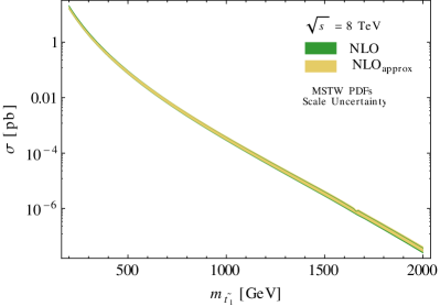 |
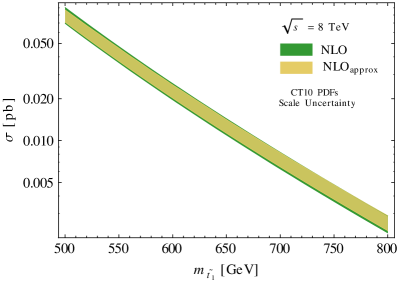
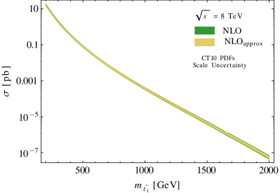
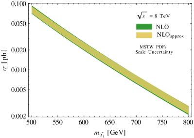
As a first step, we compare the full NLO cross section with the approximate NLO cross section given by the leading singular terms. To be specific, in the approximate NLO formulas we include the coefficients , , and in Eqs. (2.1) and (2.2), as well as those terms in which naturally arise in the SCET approach. The purpose of this comparison is to establish to what extent the leading terms in the threshold approximation reproduce the full cross section, or, in other words, if the dynamical threshold enhancement of the soft emission region takes place. This comparison is shown in Figure 2, for the case of a hadronic center of mass energy of TeV. The two rows in the figure refer to two different choices of the PDF set. NLO PDFs are employed in all of the four panels. One observes that the average of the approximate PIM and 1PI NLO formulas reproduces very well the band obtained by varying the factorization scale (which is set equal to the renormalization scale) in the full NLO result. Furthermore, the comparison in Figure 2 supports the fact that the integrals of the differential distributions in PIM and 1PI kinematics over the whole available phase space reproduce to a good accuracy the total cross section, at least for the range of stop masses of interest in this work. It is thus reasonable to expect that also the approximate NNLO formulas reproduce to a good extent the unknown full NNLO corrections.
 |
 |
 |
 |
 |
 |
 |
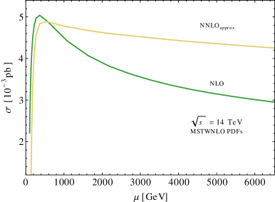 |
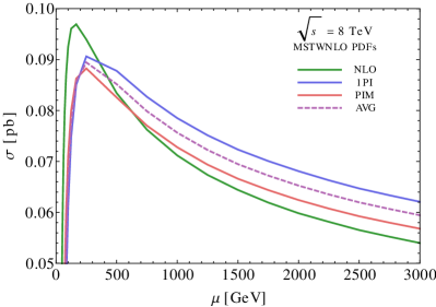
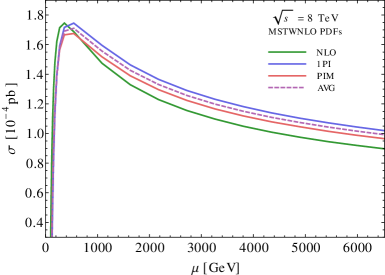
Another comparison between the scale dependence of the approximate NLO cross section and the full NLO cross section is shown in Figure 3, in which we plot separate curves for the cross section obtained in and kinematics, and for the average of the two. Both for GeV and for GeV, the scale dependence of the approximate cross sections in the range reproduces to a good extent the scale variation of the full NLO cross section in the same range.
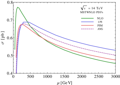
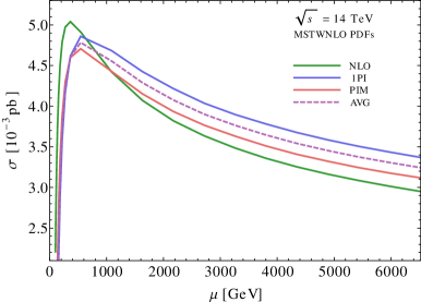
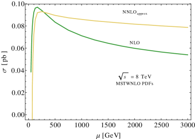
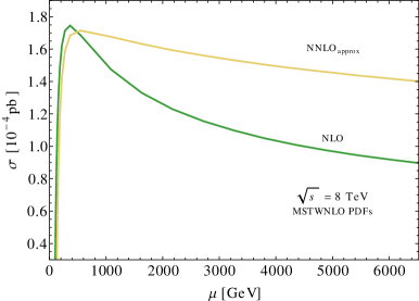
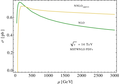
We now turn to the discussion of the approximate NNLO results, recalling first that in the approximate NNLO formulas we do not include the terms proportional to the Dirac delta functions () or () arising from the NNLO hard functions, since the scale-independent parts of the NNLO hard functions are still unknown. As expected, the approximate NNLO predictions for the pair-production cross section show a smaller scale dependence than the NLO results for the same quantity. This is illustrated in Figure 4, where two different LHC center of mass energies ( TeV and TeV) and two different stop-quark masses ( GeV and GeV) are considered. The approximate NNLO line is obtained by plotting the scale dependence of the average between the PIM and 1PI cross sections. In order to show the effect of the approximate NNLO corrections on the scale dependence, both the NLO and approximate NNLO curves are plotted using MSTW2008 NLO PDF sets. While in Figure 4 we plot exclusively the cross section scale dependence, we remind the reader that the perturbative uncertainty employed in all tables as well as in all other figures is obtained by evaluating the second and third line of Eqs. (5). Consequently, it reflects both the scale uncertainty and a kinematic scheme uncertainty, which is associated to the different sets of non-singular terms neglected in and kinematics.
| LHC TeV | MSTW2008 | |
|---|---|---|
| [GeV] | 500 | 1087.17 |
| [pb] | ||
| [pb] | ||
| [pb] | ||
| LHC TeV | CT10 | |
|---|---|---|
| [GeV] | 500 | 1087.17 |
| [pb] | ||
| [pb] | ||
| [pb] | ||
| LHC TeV | MSTW2008 | |
|---|---|---|
| [GeV] | 500 | 1087.17 |
| [pb] | ||
| [pb] | ||
| [pb] | ||
| LHC TeV | CT10 | |
|---|---|---|
| [GeV] | 500 | 1087.17 |
| [pb] | ||
| [pb] | ||
| [pb] | ||
| LHC TeV | MSTW2008 | |
|---|---|---|
| [GeV] | 500 | 1087.17 |
| [pb] | ||
| [pb] | ||
| [pb] | ||
| LHC TeV | CT10 | |
|---|---|---|
| [GeV] | 500 | 1087.17 |
| [pb] | ||
| [pb] | ||
| [pb] | ||
A more precise assessment of the impact of the approximate NNLO corrections on the central value of the cross section and on the associated perturbative uncertainty can be obtained by comparing predictions for fixed values of the stop mass. This analysis is presented in Tables 3 and 4, 5 and 6, and 7 and 8, which refer to the LHC with center of mass energies TeV, 8 TeV, and 14 TeV, respectively. In all tables we consider two different values of the lightest top-squark mass: i) the value associated to the benchmark point 40.2.5, GeV, and ii) a stop mass GeV, close to the current lower bound for this particle as determined by searches at the LHC. In all tables, the first uncertainty is perturbative, determined as explained in Eq. (5), while the second uncertainty is obtained by scanning over the 90% CL sets of the corresponding PDFs and by taking into account the error on . In particular, the PDF uncertainty is determined by seeing how the average of the PIM and 1PI predictions changes when evaluated with different members of the PDF set. The numbers for the cross sections have been obtained by employing PDFs fitted at the corresponding order: LO predictions are obtained by employing LO PDFs, NLO predictions employ NLO PDFs, and approximate NNLO predictions employ NNLO PDFs.
In all cases listed in the tables, the inclusion of the approximate NNLO corrections reduces the perturbative uncertainty, when expressed as a percentage of the central value, by more than a factor of 2 with respect to the corresponding NLO prediction. We can summarize the content of the tables as follows: the scale variation in the range can increase the NLO central value up to or lower it up to . At approximate NNLO, the scale variation can increase the central value of the cross section up to or decrease it up to . These considerations are valid both when one employs CT10 PDFs [48] or MSTW2008 PDFs.
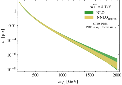
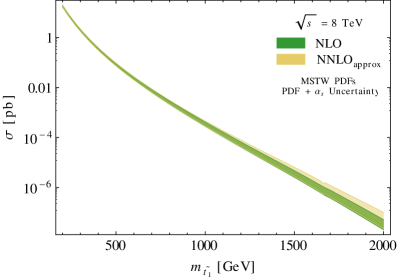
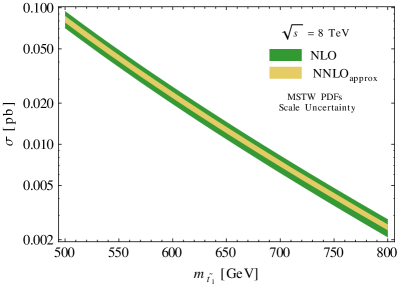
In almost all cases illustrated in the tables, the PDF and uncertainty grows marginally in the approximate NNLO predictions with respect to the NLO predictions. Another way to look at the PDF and uncertainty is shown in Figure 5, where this uncertainty band is plotted as function of the top squark mass in the range GeV at the LHC with center of mass energy of TeV. The left panel refers to the case in which CT10 PDFs are employed, while the right panel refers to the case in which the PDFs employed are MSTW2008. One sees that both bands become larger for large stop masses. The approximate NNLO band in the left panel is almost everywhere inside the NLO band, while in the right panel the approximate NNLO band is larger than the NLO band. However, the bands obtained by using CT10 PDFs remain larger than the ones obtained when using MSTW2008 PDFs.
Tables 3 to 8 also include the values for the factors at NLO and approximate NNLO, which are both normalized to the LO cross section, i.e.
| (43) |
The NLO factors tend to be slightly larger when CT10 PDFs rather than MSTW2008 PDFs are employed (roughly 1.5 vs. 1.3), but they are not very sensitive to the collider center of mass energy or to the mass of the top squark. The ratio ranges from to , therefore the approximate NNLO corrections have only a moderate impact on the central value of the NLO cross section.222In this numerical analysis we use NNLO PDFs together with our approximate NNLO results for the hard-scattering kernels. One could also make a different choice and use NLO PDFs with the approximate NNLO formulas, in that case the impact on the central values of our predictions would be bigger. For top-squark masses smaller than TeV, the central value for the approximate NNLO cross section falls well within the NLO scale uncertainty band.
 |
 |
 |
 |
 |
 |
 |
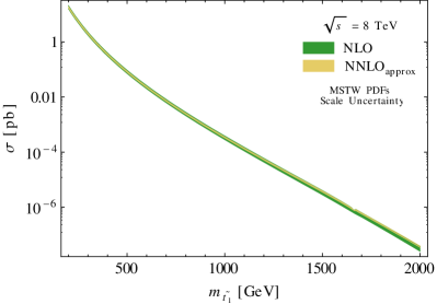 |
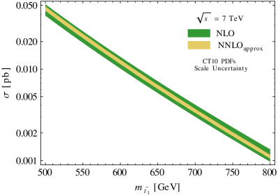
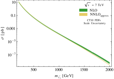
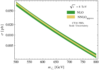
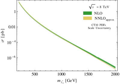
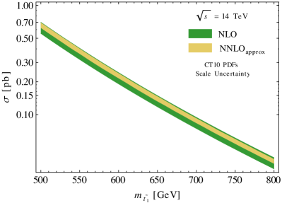
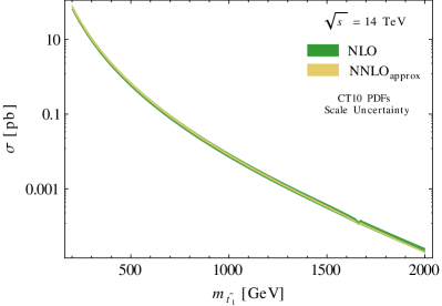
Finally, Figure 6 shows the cross section as a function of the top-squark mass up to TeV for the LHC at , and TeV center of mass energy. In all cases, the bands represent the residual perturbative uncertainties, obtained as explained above. In Figure 6 we employ CT10 PDFs. One sees that, for large values of the stop mass, the approximate NNLO band is below the NLO band at and TeV center of mass energy, while, for the LHC at TeV, the approximate NNLO band overlaps with the lower part of the NLO band. For comparison, in Figure 7 we repeat the same analysis by employing MSTW2008 PDFs for the LHC at TeV. In this case, for large stop masses the approximate NNLO scale uncertainty bands tend to be slightly above the NLO bands.
| CTEQ6.6 PDFs | GeV | GeV |
|---|---|---|
| [pb] from [7] | ||
| [pb], this work |
| CTEQ6.6 PDFs | GeV | GeV |
|---|---|---|
| [pb] from [7] | ||
| [pb], this work |
We conclude this Section by comparing our results with the ones presented in [7] and [19], which have NLO+NLL accuracy. In Tables 9 and 10 we show the results obtained for the input parameters employed in [7], which coincide with the SPS1a’ benchmark scenario of [50], as well as for two different values of the stop mass. Table 9 refers to the LHC with TeV center of mass energy while Table 10 refers to the LHC with a center of mass energy of TeV. We checked that, as expected, the NLO results in [7] coincide with the ones obtained with our modified version of Prospino. The central values of our approximate NNLO predictions for the total cross section are in very good agreement with the ones obtained by means of NLO+NLL formulas in [7]. However, the perturbative uncertainties at approximate NNLO accuracy appear to be smaller that the NLO+NLL scale uncertainties.
| [GeV] | NLO [pb] | NLL [19] [pb] | [pb] | [19] | |
|---|---|---|---|---|---|
In [19], the authors perform a simultaneous resummation of the production threshold logarithms and Coulomb singularities at NLL accuracy, including bound-state effects. Table 7 in [19] reports result for the production of top squark pairs at the CMSSM benchmark point 40.2.4 [43]. Results for higher values of the stop quark mass can be found in the files provided with the arXiv submission of [19]. Coulomb resummation and bound state effects increase the cross section, but the largest effect in the NLL results of [19] is due to soft resummation. The authors of [19] employ a private version of the MSTW2008 NLO PDFs in their calculations. In Table 11 we compare our findings with the ones of [19]. One can immediately see that our cross section prediction (inclusive of perturbative uncertainty) has a sizable overlap with the predictions quoted in [19] (inclusive of perturbative uncertainty). In all cases, the central value of our predictions falls within the perturbative uncertainty of the NLL calculations. The central values of the approximate NNLO calculations are lower than the ones of [19], as it can be seen from the fact that the quantities are lower than the corresponding quantities in [19]. In analyzing this fact it is necessary to take into account that our result does not include the additional enhancements due to Coulomb corrections, bound state effects and resummation of scale-dependent logarithms in the hard function333In our set-up, the latter would correspond to keep the contributions of the scale-dependent terms in , see Eq. (36). In this sense, it would be more natural to compare our results with the predictions labeled and in [19]; these two approaches give factors which are roughly - smaller than the ones corresponding to the NLL predictions (see Fig. 15 in [19]), and fully compatible with our results. Additionally, experience with top quark production indicates that NNLL resummation gives cross sections which are larger than the ones obtained from the corresponding approximate NNLO formulas [21, 22].
However, at this point in our discussion, the stage is set to comment on the reciprocal advantages and disadvantages of the various methods employed to implement soft gluon resummation and/or approximate NNLO formulas. This point can be better illustrated in the case of top quark pair production, where full NNLO results recently became available [51, 52]. The various calculational schemes adopted by different groups can be classified with respect to two aspects: i) The kind of kinematics employed, and ii) the space in which the resummation is carried out. Many predictions for the total top quark pair cross section are obtained by employing the traditional production threshold kinematics identified by the limit [53, 20], while PIM kinematics and 1PI kinematics, which additionally allow one to calculate differential distributions of phenomenological interest in top quark physics, are employed in [21] and [54, 22], respectively. One can then decide to work in Mellin moment space [53, 54], or in directly in momentum space [20, 21, 22]. All of these schemes allow one to obtain NNLL or approximate NNLO accuracy and they differ in the kind of formally subleading terms which are neglected. Without guidance from complete NNLO calculations there are no definitive arguments to prefer a priori one scheme to another. What one can do is to see how a given approximation does at NLO, where exact results are known, along the lines we followed at the beginning of this section. For the top quark production, all of the predictions obtained in the various schemes are compatible with each other when perturbative uncertainties are taken into account [55]. It is only a posteriori, when the results of a full NNLO calculation are available, that one can see which of the various approximate NNLO/NNLL results is closest to the exact NNLO result. In the case of the top quark total cross section, our method, based on PIM and 1PI kinematics and momentum space, provides results which are slightly lower than, but compatible with, the results of the other groups. It is important to stress that there is not a clear pattern indicating, even a posteriori, a definite methodological bias: the approximate NNLO prediction which best approximates the full NNLO total cross section is based upon 1PI kinematics and Mellin space [54], while Mellin space and momentum space calculations in the production threshold limit provide very similar results [53, 20]. A detailed analysis of the various approaches was carried out in Section 5.2 of [22]; in particular, it was shown that the approach based on SCET and employed here significantly improves the agreement between the results obtained in 1PI and PIM kinematics. Furthermore, it is possible to argue that the good numerical agreement between the exact NLO result at the LHC and the corresponding approximation based on production threshold expansion is somewhat fortuitous: In fact, in spite of the fact that the expansion fails to reproduce the correct shape of the (unphysical) distribution in the gluon fusion channel, the integral of the approximate distribution is very close to the full NLO result (see for example the discussion in [56]). On the other hand it is fair to say that the difference between the full NNLO calculation of the top production cross section and the results of [21, 22, 44] is an a posteriori indication that the neglected formally subleading terms in those works turned out to be numerically larger than the neglected subleading terms in the other approaches.
In conclusion, we believe that, in absence of a full NNLO calculation, approaches leading to different kinds of approximate NNLO /NNLL predictions are well worth exploring. Furthermore, numerical differences among predictions based on different approaches should be conservatively taken as a measure of the uncertainty associated to the neglected subleading corrections. Precisely for this reason, following the procedure of [44], we decided to base our predictions for the stop production cross section on an average of the PIM and 1PI kinematics calculations and we estimated the perturbative error not only by means of the scale variation, but also by considering the maximal difference between the predictions obtained in the two kinematic schemes, as explained in this section.
6 Conclusions
Supersymmetry is certainly one of the best motivated scenarios for physics beyond the standard model. If supersymmetry is broken just above the electroweak scale, the supersymmetric partners of the known particles are expected to have masses of the order of 1 TeV, and they could soon be observed at the LHC. For these reasons it is important to have precise theoretical predictions for the production cross sections of supersymmetric particles at hadron colliders. Top squarks are expected to be among the lightest colored supersymmetric particles, and consequently they might be the supersymmetric partners which are most easily accessible at the LHC. In this paper we have employed effective field theory techniques in order to improve existing NLO calculations for stop-pair production by evaluating higher-order perturbative corrections arising from soft-gluon emissions.
In particular, we have adopted a framework which allows one to resum large logarithmic corrections at NNLL accuracy in the stop pair production process. The resummation can be carried out in two different kinematic schemes, referred to as PIM and 1PI. In principle, this fact enables one to obtain predictions for both the pair invariant mass distribution and the top-squark and rapidity distributions, as well as for the total cross section, which is at the moment the observable of primary interest in phenomenological studies. Furthermore, by re-expanding the NNLL resummation formulas, it is possible to obtain predictions for the cross section which have approximate NNLO accuracy in fixed-order perturbation theory. The evaluation of these approximate NNLO formulas represents the main goal of this work, where we obtained analytic expressions for all of the coefficients multiplying the plus distributions in the variables and in the NNLO hard-scattering kernels for the double differential distributions in the two kinematic schemes considered. This was made possible by a complete computation of the hard-function matrices in both production channels at NLO accuracy, the calculation of which represents the main technical result of the present work.
The impact of the approximate NNLO corrections on the stop pair production cross section has been examined. In order to obtain the best possible predictions and a better control on the neglected subleading terms, we have averaged the approximate NNLO results obtained in PIM and 1PI kinematics and matched them with exact fixed-order NLO calculations. As in the case of slepton-pair production studied in [17], we found that the total cross section depends strongly on the mass of the produced particles, while the dependence on the remaining SUSY parameters, such as the masses of other supersymmetric particles, is rather weak. We have found that including the approximate NNLO predictions for the pair production cross section reduces the perturbative uncertainty by more than a factor of two with respect to the NLO results. We stress that we explicitly accounted for the kinematic scheme uncertainty arising from the use of approximate NNLO formulas and we combined it with the scale uncertainty, as explained in Section 5. It was found that the approximate NNLO corrections have only a moderate impact on the central value of the NLO total cross section. We compared our result with analogous calculations at NLO+NLL accuracy [7, 19] which were carried out by means of methods which are different from the ones employed in this work and within different kinematic schemes. We found very good agreement with the results of [7] and a substantial agreement within the quoted perturbative uncertainties with [19], although the cross section values we found tend to be slightly smaller than the ones quoted in [19]. We conclude by observing that, after the NNLO corrections are included, the main theoretical uncertainty on the total cross section comes from the PDFs. This is particular evident when large values of the stop mass are considered. Therefore, the results presented in this paper allow one to improve the precision of the stop-pair total cross section predictions by reducing their scale dependence to the extent that it becomes considerably smaller than PDF uncertainty.
Acknowledgments
We would like to thank A. von Manteuffel and S. Berge for useful discussions and T. Plehn for assistance with Prospino. The work of A.F. was supported in part by the PSC-CUNY Award No. 65214-00-43 and by the National Science Foundation Grant No. PHY-1068317. The research of M.N. is supported by the ERC Advanced Grant EFT4LHC of the European Research Council, the Cluster of Excellence Precision Physics, Fundamental Interactions and Structure of Matter (PRISMA – EXC 1098) and grant NE 398/3-1 of the German Research Foundation (DFG), grants 05H09UME and 05H12UME of the German Federal Ministry for Education and Research (BMBF), and the Rhineland-Palatinate Research Center Elementary Forces and Mathematical Foundations. L.V. acknowledges the Alexander von Humboldt Foundation for support.
Appendix A NLO soft functions
In this appendix we collect the results of the calculation of the NLO soft function in PIM kinematics [21] and in 1PI kinematics [22].
It was proven in [13] that the Laplace-transformed soft function defined in Eq. (30) is related to the position-space Wilson loop [57]. In particular, the soft function in position space is defined as (see Eq. (39) in [21])
| (44) |
where () indicates time ordering (anti-time ordering), while is the operator
| (45) |
The four soft Wilson lines are oriented along the directions of the incoming partons ( and ), and along the four-velocities of the outgoing top squarks ( and ). The precise definition of the soft Wilson lines can be found in Eqs. (22) in [21]. The Laplace transformed soft functions can be obtained from the soft functions in position space through the relation
| (46) |
Here and below, we have omitted the dependence of the soft functions on the PIM or 1PI kinematic variables and on the heavy particle masses, as well as the subscripts or indicating the channel. The expansion of in powers of the strong coupling constant is
| (47) |
At leading order the soft functions are the same both in PIM and 1PI kinematics:
| (48) |
The bare soft function at NLO in position space can be written as
| (49) |
The matrices are related to the products of color generators and are the same for both kinematics. In the quark annihilation channel they are
| (50) |
while for the gluon fusion channel one finds
| (51) |
The functions are integrals over the soft-gluon phase-space. In PIM kinematics one finds and
| (52) |
where coincides with in the limit. Furthermore , , , and
| (53) |
In 1PI kinematics one finds again that , while
| (54) | ||||
In the case of 1PI kinematics, the definition of should be changed to .
References
- [1] M. Papucci, J. T. Ruderman and A. Weiler, Natural SUSY Endures, JHEP 1209 (2012) 035 [1110.6926].
- [2] W. Beenakker, M. Kramer, T. Plehn, M. Spira and P. Zerwas, Stop production at hadron colliders, Nucl.Phys. B515 (1998) 3–14 [hep-ph/9710451].
- [3] W. Beenakker, R. Hopker and M. Spira, PROSPINO: A Program for the production of supersymmetric particles in next-to-leading order QCD, hep-ph/9611232.
- [4] W. Hollik, M. Kollar and M. K. Trenkel, Hadronic production of top-squark pairs with electroweak NLO contributions, JHEP 0802 (2008) 018 [0712.0287].
- [5] M. Beccaria, G. Macorini, L. Panizzi, F. Renard and C. Verzegnassi, Stop-antistop and sbottom-antisbottom production at LHC: A One-loop search for model parameters dependence, Int.J.Mod.Phys. A23 (2008) 4779–4810 [0804.1252].
- [6] W. Beenakker, R. Hopker, M. Spira and P. Zerwas, Squark and gluino production at hadron colliders, Nucl.Phys. B492 (1997) 51–103 [hep-ph/9610490].
- [7] W. Beenakker, S. Brensing, M. Kramer, A. Kulesza, E. Laenen et. al., Supersymmetric top and bottom squark production at hadron colliders, JHEP 1008 (2010) 098 [1006.4771].
- [8] U. Langenfeld and S.-O. Moch, Higher-order soft corrections to squark hadro-production, Phys.Lett. B675 (2009) 210–221 [0901.0802].
- [9] U. Langenfeld, Threshold Improved QCD Corrections for Stop-Antistop production at Hadron colliders, JHEP 1107 (2011) 052 [1011.3341].
- [10] U. Langenfeld, S.-O. Moch and T. Pfoh, QCD threshold corrections for gluino pair production at hadron colliders, JHEP 1211 (2012) 070 [1208.4281].
- [11] T. Becher, M. Neubert and B. D. Pecjak, Factorization and momentum-space resummation in deep-inelastic scattering, JHEP 0701 (2007) 076 [hep-ph/0607228].
- [12] T. Becher and M. Neubert, Threshold resummation in momentum space from effective field theory, Phys.Rev.Lett. 97 (2006) 082001 [hep-ph/0605050].
- [13] T. Becher, M. Neubert and G. Xu, Dynamical threshold enhancement and resummation in Drell-Yan production, JHEP 0807 (2008) 030 [0710.0680].
- [14] V. Ahrens, T. Becher, M. Neubert and L. L. Yang, Renormalization-group improved prediction for Higgs production at hadron colliders, Eur.Phys.J. C62 (2009) 333–353 [0809.4283].
- [15] V. Ahrens, T. Becher, M. Neubert and L. L. Yang, Origin of the large perturbative corrections to Higgs production at hadron colliders, Phys.Rev. D79 (2009) 033013 [0808.3008].
- [16] T. Becher and M. D. Schwartz, Direct photon production with effective field theory, JHEP 1002 (2010) 040 [0911.0681].
- [17] A. Broggio, M. Neubert and L. Vernazza, Soft-gluon resummation for slepton-pair production at hadron colliders, JHEP 1205 (2012) 151 [1111.6624].
- [18] M. Beneke, P. Falgari and C. Schwinn, Threshold resummation for pair production of coloured heavy (s)particles at hadron colliders, Nucl.Phys. B842 (2011) 414–474 [1007.5414].
- [19] P. Falgari, C. Schwinn and C. Wever, NLL soft and Coulomb resummation for squark and gluino production at the LHC, JHEP 1206 (2012) 052 [1202.2260].
- [20] M. Beneke, P. Falgari, S. Klein and C. Schwinn, Hadronic top-quark pair production with NNLL threshold resumption, Nucl.Phys. B855 (2012) 695–741 [1109.1536].
- [21] V. Ahrens, A. Ferroglia, M. Neubert, B. D. Pecjak and L. L. Yang, Renormalization-Group Improved Predictions for Top-Quark Pair Production at Hadron Colliders, JHEP 1009 (2010) 097 [1003.5827].
- [22] V. Ahrens, A. Ferroglia, M. Neubert, B. D. Pecjak and L.-L. Yang, RG-improved single-particle inclusive cross sections and forward-backward asymmetry in production at hadron colliders, JHEP 1109 (2011) 070 [1103.0550].
- [23] A. Ferroglia, M. Neubert, B. D. Pecjak and L. L. Yang, Two-loop divergences of scattering amplitudes with massive partons, Phys.Rev.Lett. 103 (2009) 201601 [0907.4791].
- [24] A. Ferroglia, M. Neubert, B. D. Pecjak and L. L. Yang, Two-loop divergences of massive scattering amplitudes in non-abelian gauge theories, JHEP 0911 (2009) 062 [0908.3676].
- [25] W. Beenakker, S. Brensing, M. Kramer, A. Kulesza, E. Laenen et. al., NNLL resummation for squark-antisquark pair production at the LHC, JHEP 1201 (2012) 076 [1110.2446].
- [26] T. Pfoh, Phenomenology of QCD threshold resummation for gluino pair production at NNLL, JHEP 1305 (2013) 044 [1302.7202].
- [27] W. Beenakker, T. Janssen, S. Lepoeter, M. Kramer, A. Kulesza et. al., Towards NNLL resummation: hard matching coefficients for squark and gluino hadroproduction, JHEP 1310 (2013) 120 [1304.6354].
- [28] N. Kidonakis, E. Laenen, S. Moch and R. Vogt, Sudakov resummation and finite order expansions of heavy quark hadroproduction cross-sections, Phys.Rev. D64 (2001) 114001 [hep-ph/0105041].
- [29] V. Ahrens, A. Ferroglia, M. Neubert, B. D. Pecjak and L. L. Yang, Threshold expansion at order for the invariant mass distribution at hadron colliders, Phys.Lett. B687 (2010) 331–337 [0912.3375].
- [30] J. C. Collins, D. E. Soper and G. F. Sterman, Factorization of Hard Processes in QCD, Adv.Ser.Direct.High Energy Phys. 5 (1988) 1–91 [hep-ph/0409313].
- [31] T. Becher and M. Neubert, Infrared singularities of scattering amplitudes in perturbative QCD, Phys.Rev.Lett. 102 (2009) 162001 [0901.0722].
- [32] T. Becher and M. Neubert, On the structure of infrared singularities of gauge-theory amplitudes, JHEP 0906 (2009) 081 [0903.1126].
- [33] T. Becher and M. Neubert, Infrared singularities of QCD amplitudes with massive partons, Phys.Rev. D79 (2009) 125004 [0904.1021].
- [34] J. Vermaseren, New features of FORM, math-ph/0010025.
- [35] C. Studerus, Reduze-Feynman Integral Reduction in C++, Comput.Phys.Commun. 181 (2010) 1293–1300 [0912.2546].
- [36] A. von Manteuffel and C. Studerus, Reduze 2 - Distributed Feynman Integral Reduction, 1201.4330.
- [37] G. Passarino and M. Veltman, One Loop Corrections for e+ e- Annihilation Into mu+ mu- in the Weinberg Model, Nucl.Phys. B160 (1979) 151.
- [38] T. Hahn and M. Perez-Victoria, Automatized one loop calculations in four-dimensions and D-dimensions, Comput.Phys.Commun. 118 (1999) 153–165 [hep-ph/9807565].
- [39] R. K. Ellis and G. Zanderighi, Scalar one-loop integrals for QCD, JHEP 0802 (2008) 002 [0712.1851].
- [40] A. van Hameren, OneLOop: For the evaluation of one-loop scalar functions, Comput.Phys.Commun. 182 (2011) 2427–2438 [1007.4716].
- [41] I. Korchemskaya and G. Korchemsky, On lightlike Wilson loops, Phys.Lett. B287 (1992) 169–175.
- [42] S. Moch, J. Vermaseren and A. Vogt, The Three loop splitting functions in QCD: The Nonsinglet case, Nucl.Phys. B688 (2004) 101–134 [hep-ph/0403192].
- [43] S. AbdusSalam, B. Allanach, H. Dreiner, J. Ellis, U. Ellwanger et. al., Benchmark Models, Planes, Lines and Points for Future SUSY Searches at the LHC, Eur.Phys.J. C71 (2011) 1835 [1109.3859].
- [44] V. Ahrens, A. Ferroglia, M. Neubert, B. D. Pecjak and L. L. Yang, Precision predictions for the t+t(bar) production cross section at hadron colliders, Phys.Lett. B703 (2011) 135–141 [1105.5824].
- [45] A. Martin, W. Stirling, R. Thorne and G. Watt, Parton distributions for the LHC, Eur.Phys.J. C63 (2009) 189–285 [0901.0002].
- [46] A. Martin, W. Stirling, R. Thorne and G. Watt, Uncertainties on in global PDF analyses and implications for predicted hadronic cross sections, Eur.Phys.J. C64 (2009) 653–680 [0905.3531].
- [47] A. Martin, W. Stirling, R. Thorne and G. Watt, Heavy-quark mass dependence in global PDF analyses and 3- and 4-flavour parton distributions, Eur.Phys.J. C70 (2010) 51–72 [1007.2624].
- [48] H.-L. Lai, M. Guzzi, J. Huston, Z. Li, P. M. Nadolsky et. al., New parton distributions for collider physics, Phys.Rev. D82 (2010) 074024 [1007.2241].
- [49] P. M. Nadolsky, H.-L. Lai, Q.-H. Cao, J. Huston, J. Pumplin et. al., Implications of CTEQ global analysis for collider observables, Phys.Rev. D78 (2008) 013004 [0802.0007].
- [50] J. A. Aguilar-Saavedra, A. Ali, B. C. Allanach, R. L. Arnowitt, H. A. Baer et. al., Supersymmetry parameter analysis: SPA convention and project, Eur.Phys.J. C46 (2006) 43–60 [hep-ph/0511344].
- [51] P. Baernreuther, M. Czakon and A. Mitov, Percent Level Precision Physics at the Tevatron: First Genuine NNLO QCD Corrections to , Phys.Rev.Lett. 109 (2012) 132001 [1204.5201].
- [52] M. Czakon, P. Fiedler and A. Mitov, The total top quark pair production cross-section at hadron colliders through , 1303.6254.
- [53] M. Aliev, H. Lacker, U. Langenfeld, S. Moch, P. Uwer et. al., HATHOR: HAdronic Top and Heavy quarks crOss section calculatoR, Comput.Phys.Commun. 182 (2011) 1034–1046 [1007.1327].
- [54] N. Kidonakis, Next-to-next-to-leading soft-gluon corrections for the top quark cross section and transverse momentum distribution, Phys.Rev. D82 (2010) 114030 [1009.4935].
- [55] N. Kidonakis, Theoretical results for top quark production, 1304.7775.
- [56] V. Ahrens, A. Ferroglia, M. Neubert, B. Pecjak and L. Yang, Top-Quark Pair Production Beyond Next-to-Leading Order, Nucl.Phys.Proc.Suppl. 205-206 (2010) 48–53 [1006.4682].
- [57] G. Korchemsky and G. Marchesini, Resummation of large infrared corrections using Wilson loops, Phys.Lett. B313 (1993) 433–440.