Higher laminations, webs and $\mathcal{N}=2$ line operators

Abstract:

A detailed study of half-BPS line operators of higher rank 4d $\mathcal{N}=2$ theory engineered from six dimensional $A_{N-1}$ $(2,0)$ theory on a bordered Riemann surface with full marked points is performed. Geometrically, each 4d UV line operator is represented by an irreducible bipartite web formed by three junctions on Riemann surface, and such web structure is called higher lamination. Algebraically, the space of UV line operators is identified with the integral tropical $a$ coordinates of the corresponding $\mbox{PGL}(\text{N,C})$ local system, and the space of IR line operator is identified with the cluster $X$ coordinates of $\text{SL}(\text{N,C})$ local system. The expectation value of UV line operator at Coulomb branch parameterized by $X$ coordinates is calculated, and the result is a positive Laurent polynomial in $X$. Using the expectation values, we calculate the operator product expansion (OPE) between the line operators, which is then represented geometrically by higher rank Skein relations. We also calculate the Poisson brackets of these line operators, and Frenchel-Nielson type coordinates are constructed for Higher Teichmuller space, etc.

1 Introduction

The line or loop operators of quantum field theory play a very important role in probing the dynamics of the theory: the expectation value of the Wilson or ’t Hooft loop of 4d gauge theory can be used to determine the phases of theory; The loop equations provide an important clue to the discovery of dual string theory [1], and Wilson loops are very important observables in the study of AdS/CFT correspondence [2, 3]; The expectation value of certain special Wilson loop is related to the scattering amplitude in 4d $\mathcal{N}=4$ super Yang-Mills theory [4, 5], etc.

We are going to study half-BPS line operators of a large class of 4d $\mathcal{N}=2$ quantum field theories engineered using 6d $A_{N-1}$ $(2,0)$ theory on a Riemann surface $\Sigma$ with various defects [6, 7, 8]. A lot of studies have been done for $A_{1}$ theory [9, 10], and they have a lot of interesting applications:

• They are important observables of 4d theory.

• A basis of them gives a nice maximal set of commuting Hamiltonian of the Seiberg-Witten (Hitchin) integrable system, which is very useful for the quantization [11, 12].

• They form a very interesting (quantum) algebra, and the Nekrasov instanton partition function is related to the quantization of this algebra [13, 14, 15, 16].

• The framed BPS states can be defined and calculated [10].

The 4d line operators of $A_{1}$ theory are derived from wrapping half-BPS surface operators of 6d theory on one cycle of Riemann surface, and the classification should be related to the classification of cycles on $\Sigma$. This picture is confirmed for Lagrangian $A_{1}$ theory in [9], which shows that 4d line operator is classified by non-intersecting closed curves on $\Sigma$. Interestingly, such set of closed curves have been studied in great detail in mathematical literature and called laminations [20]. Using lamination language, one can extend the classification to non-Lagrangian $A_{1}$ theories [10].

This paper serves as an attempt to do a systematic study about line operators of higher rank theory defined using Riemann surface $\Sigma$ with full defects (regular and irregular). Naively, the generalization is straightforward: one wrap various 6d half-BPS surface operators on closed curves to get 4d line operators. This picture seems perfectly right if we only consider the usual Wilson lines built from weakly coupled gauge group, since there is indeed 6d surface operator labeled by arbitrary irreducible representation of $\text{SU}(N)$ gauge group [21, 22, 23]. So the classification using 6d picture agrees with the result using field theory analysis [24].

However, this can not be the whole story for the following two reasons: firstly, unlike $A_{1}$ theory, there is strongly coupled matter system which carries non-trivial Coulomb branch operators, and there should be other non-trivial line operators charged on them as the usual Wilson loop is not suitable; Secondly, it is shown in [25] that webs on $\Sigma$ can also appear as the 4d line operators using 2d-4d correspondence [26].

We will confirm in this paper that the webs are necessary for the classification of 4d line operators. The important tool is the operator product expansion (OPE) between ordinary Wilson and ’t Hooft line operator, since new line operators must appear in the OPE if they exist. Remarkably, those new line operators can be represented by webs formed by simple three junctions, and a complete classification of these three junctions will be given. Using these webs and the cluster algebra tools, we are going to make following main conjectures:

• The space of 4d UV line operators is identified with the integral tropical $a$ coordinates of the moduli space of decorated $\mbox{PGL}(N,C)$ local system on $\Sigma$; The cluster $X$ coordinates of the framed $\mbox{SL}(N,C)$ local system are identified with the IR line operators, which also parameterize the Coulomb branch. This is a local description as there are a lot of cluster coordinates systems related by quiver mutations.

• The expectation value $\text{I}({\cal L})$ of a UV line operator ${\cal L}$ on Coulomb branch is calculated and expressed as a positive Laurent polynomial in cluster $X$ coordinate. The leading order term for a UV line operator with coordinates $(a_{1},\ldots,a_{n})$ is

  $$\text{I}_{A}({\cal L})=\prod X_{i}^{a_{i}}+\ldots.$$ (1)

  Using the canonical map, one can define OPE between line operators:

  $$\text{I}({\cal L}_{1})*\text{I}({\cal L}_{2})=\sum_{{\cal L}}\text{C}_{{\cal L}_{1}{\cal L}_{2}}^{\cal L}\mbox{I}({\cal L}),$$ (2)

  where the sum is finite and $\text{C}_{{\cal L}_{1}{\cal L}_{2}}^{\cal L}$ is a positive integer, and $\text{C}_{{\cal L}_{1}{\cal L}_{2}}^{{\cal L}_{1}+{\cal L}_{2}}=1$.

• We find higher rank Skein relations which give the OPEs in a geometric way.

• Using the Skein relations, any 4d half-BPS line operator can be represented by an irreducible bipartite web on $\Sigma$, and those web structures are called higher laminations. This is a global description, and the space of higher laminations is in one-to-one correspondence with the integral tropical $a$ coordinates described in first statement.

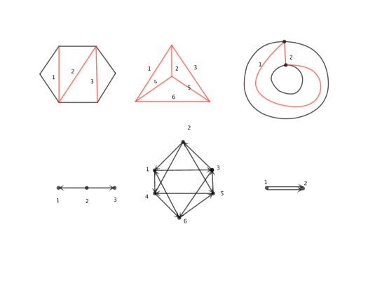
Let me explain in some detail what each statement means. As we discussed earlier, the space of UV line operators in the $A_{1}$ theory is identified with the lamination space. On the other hand, it is shown in [20] that the lamination space is in one to one correspondence with the tropical $a$ coordinates of $\mbox{PGL}(2,C)$ local system defined on $\Sigma$. The cluster $X$ coordinate is related to the one cycle on Seiberg-Witten curve, which is then naturally identified with the IR line operator [10]. Remarkably, the cluster coordinates (a quiver) for the higher rank theory defined using full defects are found in a seminal paper by Fock and Goncharov [27], i.e. the quiver for $A_{2}$ theory on once punctured torus is shown in figure. 1. Based on the analogy with $A_{1}$ theory, it is straightforward to identify the space of UV line operator as the tropical $a$ coordinate of the corresponding quiver. Here we make the definition much more precise: they actually take values $k/N$ with $k$ integer and also satisfy some special constraints (see (54) and (55) for the detailed constraints of $A_{2}$ theory.).

Figure 1: Top left: the BPS quiver for $A_{2}$ theory on once punctured torus, here the quiver nodes on the edges labeled by same red lines are identified. There is a cluster $X$ variable on each quiver node. Top right: the tropical $a$ coordinate of a line operator $L$. Bottom: the OPE between Wilson and ’t Hooft line, and a bipartite web must appear in the OPE.

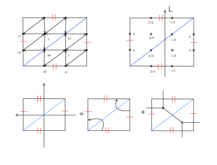
The second statement is established by studying line operator represented by closed curve on $\Sigma$: one can calculate its monodromy of $\mbox{SL}(N,C)$ local system using very simple combinatorial method [27], and the answer is always a positive Laurent polynomial in cluster $X$ coordinates, which is the expectation value of UV line operator as a direct generalization of what is proposed for $A_{1}$ case [10] (we also call it canonical map following [27].). For the closed curve L shown in figure. 1, the answer is

$$\mbox{I}(\mbox{L})={1\over{x^{2/3}y^{1/3}a_{0}^{1/3}a_{1}^{2/3}b_{0}^{1/3}b_{1}^{2/3}}}+{{b_{1}^{1/3}}\over{x^{2/3}y^{1/3}a_{0}^{1/3}a_{1}^{2/3}b_{0}^{1/3}}}+\frac{x^{1/3}b_{1}^{1/3}}{y^{1/3}a_{0}^{1/3}a_{1}^{2/3}b_{0}^{1/3}}+\frac{x^{1/3}a_{1}^{1/3}b_{1}^{1/3}}{y^{1/3}a_{0}^{1/3}b_{0}^{1/3}}+$$

$$\frac{x^{1/3}b_{0}^{2/3}b_{1}^{1/3}}{y^{1/3}a_{0}^{1/3}a_{1}^{2/3}}+\frac{x^{1/3}a_{1}^{1/3}b_{0}^{2/3}b_{1}^{1/3}}{y^{1/3}a_{0}^{1/3}}+\frac{x^{1/3}y^{2/3}a_{1}^{1/3}b_{0}^{2/3}b_{1}^{1/3}}{a_{0}^{1/3}}+x^{1/3}y^{2/3}a_{0}^{2/3}a_{1}^{1/3}b_{0}^{2/3}b_{1}^{1/3}.$$ (3)

These canonical maps have two remarkable applications: firstly the tropical $a$ coordinates of this line operator can be read from the exponent of leading order term, see figure. 1; Secondly it can be used to define the OPE between line operators: we simply multiply canonical maps of two line operators and the answer should be expanded into the sum of canonical map of other line operators. Using the OPE, we find that the usual Wilson loops are classified by the irreducible representation of the $\text{SU}(N)$ group, and the OPE between them has the same support as the corresponding tensor product of irreducible representations. This strongly suggests that our results are correct.

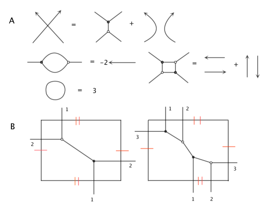
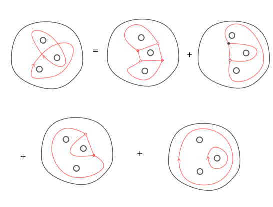
Most interestingly, by doing OPE between the usual Wilson and ’t Hooft line operators, we find extra line operator which is naturally described as a web formed by two three junctions, see figure. 1. We classify all the three junctions of any higher rank theory, and any 4d half-BPS line operator can be represented by the webs formed by three junctions. These web structures are called higher laminations in direct analogy with the $A_{1}$ case; Some webs on torus are shown in figure. 2. This description is independent of the cluster coordinates system and is the geometric picture for 4d line operators of higher rank theory. In general, the OPE between any line operators can be found geometrically using local Skein relations, see figure. 2 for $A_{2}$ theory. Such Skein relations are also important for the classification of webs: we only consider irreducible webs which can not be reduced by Skein relations.

Figure 2: A: Skein relations for $A_{2}$ theory. B. Bipartite webs on once punctured torus of $A_{2}$ theory, and edges of three junctions with same label are connected.

There are some compelling evidences supporting our results: Poisson brackets for the line operators of $A_{2}$ theory on once punctured torus are calculated, and the answer is in perfect agreement with the underlying integrable system: there are three commuting Hamiltonians, etc. There are theories which can be engineered either using $A_{1}$ or $A_{2}$ theory, and the canonical map of same line operator agrees with each other perfectly!

This paper is organized as follows: in section II, we review some basic facts of line operators of $A_{1}$ theory, and we emphasize a coherent picture of geometric and algebraic descriptions. In section III, we carry out a detailed study of line operators for theories defined on once punctured torus, and find the basic three junctions, Skein relations, etc. Section IV gives a brief description for line operators of theories defined on general Riemann surface. Finally, a conclusion is given in section V. Technical details about how to calculate monodromy is given in appendix A, and we collect some useful canonical maps in appendix B.

2 $A_{1}$ theory: line operator and lamination space

This section is a review about the line operators for $A_{1}$ theory. The geometric picture for the classification is the so-called lamination, and the algebraic picture is the tropical cluster algebra [20]. Physically, the geometric picture for the Lagrangian $A_{1}$ theory is discovered in [9] using field theory , and then extended to the non-Lagrangian theory using lamination in [10]. We are also going to discuss the canonical map, OPE, etc, and all of which will be generalized to the higher rank case in the following sections.

Let’s first say a couple of words about the four dimensional $\mathcal{N}=2$ theory we have: we start with a six dimensional $A_{1}$ $(2,0)$ theory and compactify it on a Riemann surface $M_{g,b_{i},p_{j}}$, here $b_{i}$ denotes $i$th irregular singularity and $p_{j}$ denotes the $j$th regular singularity . The IR limit is a four dimensional UV complete theory (conformal or asymptotical free theory). The UV deformations are encoded in the geometric description: the dimensionless gauge coupling is identified with the complex structure moduli of the Riemann surface; the mass parameters are the coefficients of the first order pole of regular and irregular singularity; the dimensional couplings are the coefficients of the higher order pole of the irregular singularity. The IR description can also be easily found from this geometric description: a Hitchin equation with specific boundary conditions at the singularity is defined on $M_{g,b_{i},p_{j}}$, and the spectral curve of the Hitchin moduli space is identified with the Seiberg-Witten curve of 4d theory.

The weakly coupled gauge group description is described by degeneration limit of the Riemann surface: the long tube in the degeneration limit is associated with the gauge group and other components are the matter system . The basic building blocks (matter contents) are:

• Tri-fundamental represented by a sphere with three regular singularities.

• $\mbox{D}_{N}$ type Argyres-Douglas theory represented by an sphere with one irregular singularity and one regular singularity .

The first piece is free while the second one is a strongly coupled isolated SCFT, see figure. 3A. Each regular singularity carries a $\text{SU}(2)$ flavor symmetry, and the weakly coupled gauge group description of the four dimensional theory is derived by gauging these $\text{SU}(2)$ flavor symmetries, see figure. 3B. Different duality frames correspond to different decompositions of the full Riemann surface into the above two pieces, which is a remarkably simple description of S duality [6].

Figure 3: A: The two basic matter systems for four dimensional theory built from six dimensional $A_{1}$ theory: the tri-fundamental represented by a sphere with three regular singularity and the D type Argyres-Douglas theory represented by a sphere with one irregular and one regular singularity. B: In one weakly coupled gauge group duality frame, the theory is formed by gluing above two pieces together: physically this is achieved by gauging the diagonal flavor symmetries. C: We replace each irregular singularity with a boundary with marked points.

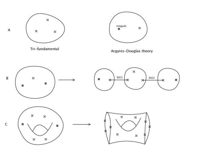
For various applications below, we need to replace an irregular singularity with a boundary plus marked points whose number depends on the type of singularity, which can be seen by studying the Stokes phenomenon around the irregular singularity, see [28]. Therefore, we are going to consider a bordered Riemann surface $\mbox{M}_{g,b_{i},n}$, here $g$ is the genus of the Riemann surface, $b_{i}$ is the number of marked points on the $i$th boundary, $n$ is the number of bulk marked points, see figure. 3C. The Coulomb branch dimension of the 4d theory is

$$n_{r}=n+\sum_{i}[{b_{i}-3\over 2}]+3g-3,$$ (4)

where $[{b_{i}-3\over 2}]$ means taking the integer part of the number inside the bracket.

Each regular puncture contributes a mass parameter (as it carries a $SU(2)$ flavor symmetry.), and each boundary with even number of marked points also contributes a mass parameter (since it carries a $U(1)$ flavor symmetry.), and the rank of the charge lattice is

$$R=2n_{r}+n_{f}=3n+\sum_{i}b_{i}+6g-6.$$ (5)

We also pick an anti-clockwise orientation for each boundary (the bulk puncture can be thought of as a boundary without any marked point.). A bordered Riemann surface with anti-clockwise orientation for each boundary is the geometric avatar for our study of line operators.

2.1 UV and IR line operator: geometric picture

The 4d theory always has a Lagrangian description for bordered Riemann surface $M_{g,0,n}$, so one can use field theory tools to study its half-BPS line operator. For a four dimensional $\mathcal{N}=2$ gauge theory with gauge group G, the Wilson operators are labeled by irreducible representations R of G and take the form

$$\mbox{W}_{\mbox{R}}=\mbox{Tr}_{\mbox{R}}\mbox{P}\int\exp(iA+\mbox{Re}\phi ds),$$ (6)

where $\phi$ is a complex scalar in the vector multiplet and ds is the line element determined by the metric. If the integral is taken along a straight line or a circle in flat $R_{4}$, this Wilson line preserves a half of $\mathcal{N}=2$ supersymmetry. Equivalently, the Wilson line operator is classified by the highest weight in the weight lattice $\Lambda_{G}$ of the gauge group $G$. The ’t Hooft operator is a disorder operator and defined by specifying the singular behavior of various fields around the loop or line in the space time:

$$F=-{B\over 2}\sin\theta d\theta\wedge d\phi,~{}~{}~{}\phi\sim i{B\over 2r},$$ (7)

and the line operator is classified by the highest weight in the coweight lattice in $\Lambda_{\hat{G}}$, or the weight lattice of Langlands dual group $\hat{G}$. For general Wilson-’t Hooft line operators, Kapustin found that the line operators are classified by the following data [24]:

$$(\mu,\nu)\in\Lambda_{cw}\times\Lambda_{w},~{}~{}~{}(\mu,\nu)\sim(\omega.\mu,~{}\omega.\nu),~{}~{}\omega\in W,$$ (8)

where $W$ is the Weyl group. The allowed magnetic weight has to satisfy the Dirac quantization condition in the presence of matter fields. Moreover, when the flavor symmetry is available, one can introduce the background gauge field for these flavor symmetries and consider the line operator carrying magnetic charge on it.

Let’s apply the above general classification to the theory defined by Riemann surface $M_{g,0,n}$, namely a Riemann surface with $n$ regular punctures. There are $3g-3+n$ gauge groups and $n$ mass parameters, and a duality frame is described by a pants decomposition of the Riemann surface (since there is only tri-fundamental matter.). The line operator is labeled by $(6g-6+3n)$ integers

$$(p_{1},p_{2},\ldots,p_{3g-3+2n};q_{1},q_{2},\ldots,q_{3g-3+n}).$$ (9)

The Weyl transformation acts as $(p_{j},q_{j})\rightarrow(-p_{j},-q_{j})$ for $j=1,2,\ldots,3g-3+n$, and $p_{j}\rightarrow-p_{j}$ for $j=3g-2+n,\ldots,3g-3+2n$. Using Weyl transformation, we may take $p$ to be positive, and they are the magnetic charges, so they have to satisfy the condition $p_{i}+p_{j}+p_{k}\in 2Z$ for three gauge groups coupled to a single pants, since the matter from the pants has to satisfy the Dirac quantization condition.

Figure 4: The Dehn-Thurston coordinates of a set of closed curves are defined using a pants decomposition: the $p_{i}$ coordinates are defined by simply counting the weighted intersecting number, while the $q_{i}$ coordinates are defined by counting the oriented winding number.

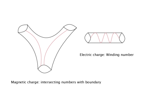
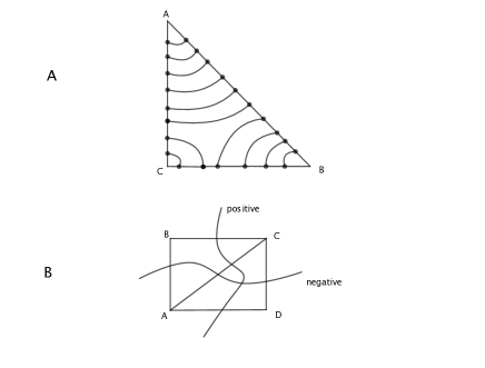
Using above field theory results, it is shown in [9] that the space of line operators are identified with the space of self- and mutually nonintersecting unoriented closed curves on $M_{g,0,n}$. Therefore, instead of studying the line operator from 4d field theory point of view, we can just study these closed curves on the Riemann surface. Now let’s start with a collection of closed curves (non-intersecting) with positive integer weights , and one can construct a set of Dehn-Thurston coordinates based on the pants decomposition: the coordinates $p_{i}$ (always positive) on a boundary circle of the pants is defined by counting the weighted intersection number, and the $q_{i}$ coordinates (it can be positive and negative depending on the winding direction) on a tube are defined by counting the winding number of the curves, see figure. 4. On the other hand, given a set of coordinates based on pants decomposition, one can easily find a set of closed curves by doing the inverse construction: one put $p_{i}$ marked point on the $i$ th boundary of the pants, and connect them pairwise without intersection on each pant (which is possible if they satisfy the condition $p_{i}+p_{j}+p_{k}\in 2Z$ on each pant, and the construction is unique), and also the number of winding on the tube is determined by the coordinates $q_{i}$, and we construct a set of non-intersecting closed curves with weight. Finally we combine the closed curves in same homotopy class, which will give back a geometric objects.

The above Dehn-Thurston coordinates are directly related to the field theory description [9], however, it has several disadvantages: firstly, the transformation of the coordinates is quite complicated under the change of pants decomposition corresponding to the S duality; Secondly, there is no pants decomposition for the Riemann surface with boundaries and the above definition of the line operator is not applicable. In next subsection, we are going to introduce another set of coordinates based on the triangulation of the Riemann surface, and the coordinates has simple transformation rule under the change of the triangulation, moreover, the definition can be extended to all bordered Riemann surface.

2.1.1 UV line operators: lamination and its coordinates

The set of the non-intersecting closed curves are called laminations in the mathematics literature [20], so space of line operator of 4d theory is naturally identified with the lamination space. Let’s now introduce the precise definition of Lamination on bordered Riemann surface. Before that, let’s give the definition of special curves: a curve is called special if it can be contracted to a bulk marked point or a boundary marked point, and a curve is contractible if it can shrink to single point which is not a marked point. Now let’s spell the definition of the Lamination:

Definition: A integral A-lamination on a bordered Riemann surface is a homotopy class of a collection of finite number of self- and mutually nonintersecting unoriented curves either closed or connecting two points of the boundary disjoint from marked points with integral weights and subject to the following conditions and equivalence relations.

(1) Weights of all curves are positive, unless a curve is special.

(2) A lamination containing a curve of weight zero is considered to be equivalent to the lamination with this curve removed.

(3) A lamination containing a contractible curve is considered to be equivalent to the lamination with this curve removed.

(4) A lamination containing two homotopy equivalent curves with weights $u$ and $v$ is equivalent to the lamination with one of these curves removed and with the weight $u+v$ on the other.

Figure 5: A: Laminations on an annulus with one marked points on each boundary, which represent the pure $SU(2)$ theory. B: Constructing coordinates for the lamination using the triangulation.

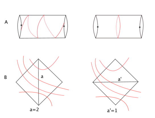
Notice that the weights for the curves around the marked points can be either positive or negative, while the other curves always have positive weights. An example of lamination on an annulus with one point on each boundary is shown in figure. 5. Instead of constructing coordinates using the pants decomposition, we use the ideal triangulation whose vertices are the marked points. An ideal triangulation is formed by simple curves whose ending points are the marked points, equivalently one can use a quiver to encode the triangulations of the internal edges, and this quiver is actually the BPS quiver [29]. An important fact is that the number of internal edges in the triangulation is $6g-6+b+3p$ which is exactly the same number of the charge lattice We give some example of triangulations and quivers for various bordered Riemann surface in figure. 6, more details about the ideal triangulation can be found in [30]. Given a lamination and a triangulation, we can construct the coordinates (labeling) for the lamination using the following simple formula:

$$a_{E}={1\over 2}\sum_{i}\omega_{i},$$ (10)

where the sum is over all the curves intersecting with the curves, see figure. 5B. The coordinates are called tropical $a$ coordinates and taking half-integer values.

Figure 6: Top: The ideal triangulations of bordered Riemann surface: disc with six marked points, sphere with four punctures, and annulus with one marked points on each boundary. Bottom: the corresponding quiver.

On the other hand, given a set of constrained half-integers (the constraints will be spelled later) on each edge of the triangulation, we can construct a lamination. First of all, we can assume all the coordinates are positive, since if some of the coordinates of $a_{i}$ is negative, we can first shift all the coordinates by a positive integers $\omega$ such that $a_{i}^{{}^{\prime}}=a_{i}+\omega$ are all positive. If we can construct lamination $L^{{}^{\prime}}$ for $a_{i}^{{}^{\prime}}$, we can add closed curves with weight $-\omega$ around each marked point to $L^{{}^{\prime}}$ (these curves will not intersect with $L^{{}^{\prime}}$) to get the lamination $L$ for the coordinates $a_{i}$. So let’s start with positive half-integer coordinates $\tilde{a}_{E}$ which satisfy the following two conditions for the coordinates on a triangle:

$$|\tilde{a}_{\alpha}-\tilde{a}_{\beta}|<\tilde{a}_{\gamma}<\tilde{a}_{\alpha}+\tilde{a}_{\beta}$$

$$\tilde{a}_{\alpha}+\tilde{a}_{\beta}+\tilde{a}_{\gamma}\in z.$$ (11)

Now for each edge in the triangle $<ABC>$, we put $2\tilde{a}_{\alpha}$ number of points on it, and for a triangle, we connect these points pairwise such that there is no intersections. The construction is unique, since we can divide the marked points on each edge into the two parts as (and the coordinates on each edge are $(AB,BC,CA)=(\tilde{a}_{\gamma},\tilde{a}_{\beta},\tilde{a}_{\alpha})$):

$$a+b=2\tilde{a}_{\gamma}~{}~{}\rightarrow~{}~{}~{}~{}~{}~{}~{}a=\tilde{a}_{\alpha}+\tilde{a}_{\gamma}-\tilde{a}_{\beta}$$

$$a+c=2\tilde{a}_{\alpha}~{}~{}~{}~{}~{}~{}~{}~{}~{}~{}~{}~{}~{}~{}b=\tilde{a}_{\beta}+\tilde{a}_{\gamma}-\tilde{a}_{\alpha}$$

$$b+c=2\tilde{a}_{\beta}~{}~{}~{}~{}~{}~{}~{}~{}~{}~{}~{}~{}~{}~{}c=\tilde{a}_{\alpha}+\tilde{a}_{\beta}-\tilde{a}_{\gamma},$$ (12)

and the solutions are positive integers due to the constraint (11), and they determine how to connect the points on the boundary of the triangles: i.e. there are $a$ curves around vertex $A$.

Figure 7: A: Given a set of tropical $a$ coordinates on a triangle, one can construct a set of non-intersecting curves, here the coordinates are $(AB,BC,CA)=(5,3,4)$. B: The rule for determining the tropical $x$ coordinate.

The ideal triangulations are not unique, and different triangulations are related by the local moves called flip (see figure. 5). The $a$ coordinates change in a very simple way under the flip:

$$a_{e}^{{}^{\prime}}=-a_{e}+max(a_{a}+a_{c},a_{b}+a_{d}).$$ (13)

If there is a boundary, one need to put further constraints on the $a$ coordinates: the coordinates on the boundary edge of the triangulation should be zero. The reason for this further constraint is that the external edge is not included in our description of $\mathcal{N}=2$ theory, as the number of internal edges are exactly equal to the rank of the charge lattice.

One might be curious about the strange constraint (11), and the reason is that these coordinates are actually the tropical $a$ coordinate of the $\text{PGL}(2,C)$ local system, which is the Langlands dual group of $\text{SL}(2,C)$. We assume that there is a $\text{SL}(2,C)$ Hitchin system on the Riemann surface for the 4d field theory description , and the line operator is taking value on the tropical $a$ coordinates of $\text{PGL}(2,C)$ local system. For more discussion on the global issue about the gauge group, see the appendix of [7].

One can construct another set of coordinates for the lamination . The definition is the following: pick a vertex of the diagonal edge of the quadrilateral and name it as $A$, then label the other vertices as $B,C,D$ in clockwise direction; if a curve goes through $AB$ and $CD$, its coordinate is positive, and the coordinates is negative if it goes through $AD$ and $BC$, see figure. 7. One can check that the $x$ and $a$ coordinates are related by the following simple formula

$$x_{i}=-\epsilon_{ij}a_{j}.$$ (14)

where $\epsilon_{ij}$ is the antisymmetric tensor read from the quiver. These $x$ coordinate is always integer, and can be both positive and negative even for the non-trivial closed curves.

2.1.2 IR line operator: one cycle on Seiberg-Witten curve

The UV theory is described by compactifying 6d theory on a punctured Riemann surface, and the lamination on Riemann surface $\Sigma$ will give us the UV line operator. From M theory picture, we have a 4d theory on two M5 branes, and M2 brane ending on M5 branes (wrap on lamination on $\Sigma$) gives 4d line operators. What about the IR line operator? In the IR limit, these multiple M5 branes become a single M5 brane compatified on another Riemann surface $\Sigma^{c}$ which is identified with the Seiberg-Witten curve [31]. It is natural to expect that M2 brane wrapped on various one cycle of $\Sigma^{c}$ will give us IR line operators.

There is actually a distinguished basis on these one cycles based on the ideal triangulation of the Riemann surface $\Sigma$. The construction goes as follows: first of all, we can replace the triangulation by a bipartite network as suggested in [32]. Usually one associate a face variable $X_{i}$ to each face in the original bipartite network, and one can read a quiver from the network. Given a bipartite network on a Riemann surface, one can construct a conjugate Riemann surface $\Sigma^{c}$ using the so-called untwisting procedure, which is quite familiar in the dimer study, see [33]. The details are not important for us, and we want to point out the crucial point: since the boundary of the face of network on $\Sigma$ becomes the one cycle on $\Sigma^{c}$, which will give a IR line operator. It is then natural to interpret the face variable $X$ as the expectation value of the IR line operators . On the other hand, these one cycles on the SW curve is also used to parameterize the Coulomb branch through the famous Seiberg-Witten construction, so the cluster $X$ coordinates not only represent the IR line operator but parameterize the Coulomb branch of 4d theory!

2.2 UV and IR line operator: algebraic picture

Geometrically, the 4d line operator is related to the weighted closed curves on the Riemann surface. Its tropical $a$ and $x$ coordinates can be constructed using the triangulation and their transformation property under the change of triangulation is simple . In fact, the above picture can be put into a general algebraic picture called (tropical) cluster algebra [34, 20].

The (tropical) cluster algebra consists a family of seeds $(\epsilon_{ij},x_{i},a_{i})$, here $\epsilon_{ij}$ is an antisymmetric matrix which can be represented by a quiver, and $x_{i}$ and $a_{i}$ are rational, real or integral numbers associated with each quiver node. Different seeds are related by the so-called mutations. The mutation acting on the quiver is

$$\epsilon^{{}^{\prime}}_{ij}=\left\{\begin{array}[]{c l}-\epsilon_{ij}&\text{if}~{}i=k~{}or~{}j=k\\ \epsilon_{ij}+\text{sgn}(\epsilon_{ik})[\epsilon_{ik}\epsilon_{kj}]_{+}&\text{otherwise}\end{array}\right.$$ (15)

The quiver mutations can be represented beautifully using the quiver diagram: A quiver is a directed graph where multiple arrows between two vertices are allowed, which is derived using $\epsilon_{ij}$ as follows: attach a quiver node for $i=1,\ldots n$, and there are $\epsilon_{ij}$ arrows between node $i$ and node $j$ . The quiver mutation for a quiver without one and two cycles (such quiver is called 2-acyclic) is defined as the following: Let Q be a quiver and k a vertex of Q. The mutation $\mu_{k}(Q)$ is the quiver obtained from Q as follows, see figure. 8:

1) for each sub quiver $i\rightarrow k\rightarrow j$, create a new arrow between $ij$ starting from $i$;

2) we reverse all arrows with source or target k;

3) we remove the arrows in a maximal set of pairwise disjoint 2-cycles.

Figure 8: The quiver mutation.

In changing the triangulation, the quiver is changed as quiver mutation (Seiberg duality), and the coordinates are changed in following way

$$a^{{}^{\prime}}_{k}=max(a_{k}{[\epsilon_{ik}]_{+}},a_{i}{[-\epsilon_{ik}]_{+}})-a_{k}$$ (16)

$${x}_{j}^{{}^{\prime}}=\left\{\begin{array}[]{c l }-{x}_{k}&if~{}j=k\\ x_{j}+\epsilon_{kj}max(x_{k},0)&if~{}\epsilon_{kj}\geq 0\\ x_{j}+\epsilon_{kj}max(-x_{k},0)&if~{}\epsilon_{kj}\leq 0\\ \end{array}\right.$$ (17)

The ordinary cluster algebra consists of also triples $(\epsilon_{ij},X_{i},A_{i})$ which are related by quiver mutations, where $\epsilon_{ij}$ is the same as the one used above and it has the same form as quiver mutations. The transformation of the $X$ coordinates under mutation is

$${X}_{j}^{{}^{\prime}}=\left\{\begin{array}[]{c l}{X}_{k}^{-1}&if~{}j=k\\ {X}_{j}(1+{X}_{k}^{-sgn(\epsilon_{jk})})^{-\epsilon_{jk}}&if~{}j\neq k,\end{array}\right.$$ (18)

and the $A$ coordinates transform in following way

$$A^{{}^{\prime}}_{k}={\prod A_{i}^{[\epsilon_{ik}]_{+}}+\prod A_{i}^{[-\epsilon_{ik}]_{+}}\over A_{k}}.$$ (19)

A two form can be defined on $A$ space

$$\omega=\epsilon_{ij}d\log A_{i}\wedge d\log A_{j};$$ (20)

and a degenerate Poisson structure can be defined on the $X$ space:

$$[X_{i},X_{j}]=\epsilon_{ij}X_{i}X_{j}.$$ (21)

These structures are compatible with the cluster transformation, i.e. if you express $(X_{i},\epsilon_{ij})$ in terms of $(X_{i}^{{}^{\prime}},\epsilon_{ij}^{{}^{\prime}})$ using the cluster transformation rule, and you will get the same form expressed in terms of $(X_{i}^{{}^{\prime}},\epsilon_{ij}^{{}^{\prime}})$.

The above two types of coordinates are related by the so-called tropification procedure. Here let’s describe a little bit about the idea of tropification, i.e. the triple $(\epsilon_{ij},x_{i},a_{i})$ can be thought of as the tropical limit of $(\epsilon_{ij},X_{i},A_{i})$. Let’s explain a little bit of tropification: the tropification about a polynomial $3a^{3}+a^{2}b+1$ is $\text{max}(3a,2a+b,0)$; more generally, for a rational function without subtraction, the tropification is

$$\text{Trop}(f(a_{1},a_{2},\ldots,a_{n}))=lim_{\epsilon\rightarrow\infty}\epsilon log(f(e^{\epsilon a_{1}},e^{\epsilon a_{2}},\ldots,e^{\epsilon a_{n}})).$$ (22)

It is then easy to see that $(\epsilon_{ij},x_{i},a_{i})$ is a tropification of $(\epsilon_{ij},X_{i},A_{i})$ by comparing their transformation property under the mutation.

2.3 Canonical map: relating UV and IR line operators

Classically it is natural to identify the expectation value of a UV line operator as the length of the closed curves on the Riemann surface, and the length should depend on the Coulomb branch, which is parameterized by the cluster $X$ coordinates. There is a remarkably simple method to calculate the length: it is related to the monodromy around the curve in the $\text{SL}(2,C)$ local system, and the monodromy can be calculated using very simple combinatorial methods [20]. Basically, one first construct a dual graph from the ideal triangulation: put a trivalent vertex inside each triangle and glue them together using the triangulation. Then put a square around each edge and a hexagon around each vertex, and this structure is called as monodromy graph. The orientation of edges in monodromy graph is chosen as following: the edges on the cycles around the marked points are taken to be in anti-clockwise direction, and the edges in hexagon is required to be in clockwise direction which can be used to fix the orientation of remaining edges.

There are three types of edges in the monodromy graph: S edge which intersects with the dual graph, E edge which is parallel with the dual graph, and finally the F edge which is inside the triangle, see figure. 9. We associate the following matrices with the three types of edges:

$$S=\begin{pmatrix}0&-1\\ 1&0\end{pmatrix},E=\begin{pmatrix}X&0\\ 0&1\end{pmatrix},F=\begin{pmatrix}1&0\\ 1&1\end{pmatrix}.$$

Figure 9: Top: the dual graph and the monodromy graph are built from the triangulations. Middle: One triangulation has three edges labeled by $a,b,c$, and the opposite edges are identified. We also draw various closed curves, and the quiver. Bottom: the Skein relations.

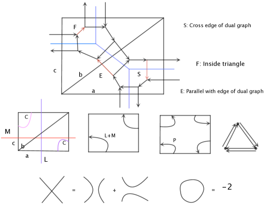
If a path is going opposite direction to the prescribed orientation for an edge, we simply use the inverse matrix. It can be checked that the monodromy around the square and the hexagon is an identity matrix up to a scalar, therefore it defines a $\text{PGL}(2)$ local system. Now the monodromy of a closed curve C is found as following: find a closed path on the monodromy graph which is in the same homotopy class as C, and then multiplying the matrices of segments in this path which will give the monodromy. For our purpose, a $\text{SL}(2)$ local system is required and the monodromy $M$ is defined as

$$M=|\text{det}(M_{0})^{-1/2}M_{0}|,$$ (23)

here $M_{0}$ is the monodromy using the above prescription and we take the absolute value to make all the expressions positive. Using the monodromy, the expectation value of the UV line operator or canonical map for curves in lamination are

• For a non-special closed curve $l$ with weight $k$, the canonical map is $\text{I}(l)=\text{Tr}(\text{M}^{k})$.

• For a special curve $l$ with positive (negative) weight $k$, the canonical map is to take the highest (lowest) eigenvalue of $\text{M}^{|k|}$. For example, the eigenvalues of the monodromy matrix have the following form (winding once):

  $$(\prod X_{i}^{1/2},\prod X_{i}^{-{1/2}}),$$ (24)

  and we define the canonical map of curve with weight one as $\text{I}(l^{+})=\prod X_{i}^{1\over 2}$ and the curve with weight minus one as $\text{I}(l^{-})=\prod X_{i}^{-{1\over 2}}$.

• For a curve connecting two points on the boundary, the canonical map is defined as:

  $$\text{I}(l)=\begin{pmatrix}1&0\\ \end{pmatrix}*\text{M}*\begin{pmatrix}1\\ 0\end{pmatrix},$$ (25)

  here the definition of $M$ is subtle as there are two choices for the starting and ending edges of the path $l$ in the monodromy graph. Our prescription is that the starting and ending edge of $l$ has the same orientation as the curve.

• For the line operator with $0$ coordinate, the canonical map is $\text{I}(0)=2$.

• For a lamination $l$ consists of many curves $l_{i}$, and the canonical map is defined as

  $$\text{I}(l)=\prod_{i}\text{I}(l_{i}).$$ (26)

Example: Let’s apply the above discussion to the theory defined by an once punctured torus, which represents the so-called $\text{SU}(2)$ $\mathcal{N}=2^{*}$ theory. The triangulation and the quiver is shown in figure. 9, and there are three quiver nodes. There are three non-trivial homology cycles which we call $L,M,C$, and the line operator associated with this three cycles has tropical $a$ coordinates $(\frac{1}{2},\frac{1}{2},0),(0,\frac{1}{2},\frac{1}{2}),(\frac{1}{2},0,\frac{1}{2})$, and the canonical map is found to be

$$I(L)={1\over\sqrt{ab}}+\sqrt{{b\over a}}+\sqrt{ab},~{}I(M)={1\over\sqrt{bc}}+\sqrt{{c\over b}}+\sqrt{bc}$$

$$I(C)={1\over\sqrt{ca}}+\sqrt{{a\over c}}+\sqrt{ac},~{}I(L+M)=\frac{2\sqrt{ac}}{a}+\frac{\sqrt{ac}}{ab}+b\sqrt{ac}+\frac{b\sqrt{ac}}{a}+\frac{\sqrt{ac}}{abc}$$

$$I(P^{+})=abc,~{}~{}I(P^{-})=a^{-1}b^{-1}c^{-1},$$ (27)

here $L+M$ is the cycle shown in figure. 9. One can calculate the OPE using the canonical map: let’s multiple the canonical map of two line operators, and expand the answer in terms of the canonical map of other line operators. A simple example is

$$I(L)*I(M)=I(L+M)+I(C),$$ (28)

Geometrically, the OPE can be found using the Skein relation, see figure. 9, and the above OPE can be easily found using Skein relations. Here are some properties for the canonical map $I(l)$ (for more details, see [27]):

• The canonical map is a Laurent polynomial in $X_{i}$ with positive integer coefficient, and the leading order term for a line operator with coordinates $a_{i}$ is $\prod X_{i}^{a_{i}}$.

• There is an OPE between line operators $\text{I}(l_{1})\text{I}(l_{2})=\sum_{l}C_{l_{1}l_{2}}^{l}\text{I}(l)$, here $C_{l_{1}l_{2}}^{l}$ is a positive integer, with $C_{l_{1}l_{2}}^{l_{1}+l_{2}}=1$.

• The Poisson structure between line operators can be easily calculated using the canonical map and the Poisson structure of cluster $X$ coordinates.

2.4 Summary

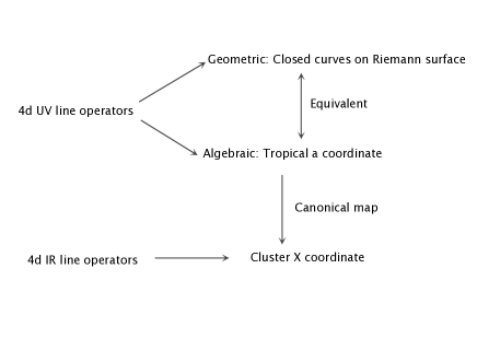
Let’s summarize the important facts about $A_{1}$ line operators (see figure. 10):

Figure 10: The basic picture of $A_{1}$ line operators.

• Each 4d UV line operator is represented by a lamination, which is a global description.

• One can parameterize the UV line operator using the cluster algebra and tropical $a$ coordinates: given a lamination, one can construct its coordinates; and given a set of coordinates, one can construct a lamination. This description is local as there are a lot of ideal triangulations.

• The space of IR line operator is identified with the cluster $X$ coordinate.

• There is a canonical map $\mbox{I}(l)$ between the lamination space and the cluster $X$ coordinates, and there is an OPE between them, which has very interesting property.

3 $A_{N-1}$ theory: torus with one full puncture

We are going to generalize the story of $A_{1}$ line operators to $A_{N-1}$ theory defined using full regular and irregular singularities. Similarly one can replace the irregular singularity with a boundary with full marked points, and the geometric object is still a bordered Riemann surface (see [28] for the exact correspondence between the bordered Riemann surface and the physical 4d $\mathcal{N}=2$ theory). In the $A_{1}$ case without the boundary, the field theory tools are available since the theory has Lagrangian description, which provides a lot of informations. Now although the weakly coupled gauge group description is still valid and can give us some clues, there are always strongly coupled matter and it is clear new phenomenon must appear.

On the other hand, the geometric picture we learned from $A_{1}$ case is still valid, and closed curves on Riemann surface should still give 4d line operators. However, it should be clear that this is not enough as each closed curve give a weakly coupled gauge group, and these line operators can not be used to probe the strongly coupled matter part.

We do have the cluster algebra tools on hand, so it is straightforward to argue that the UV line operators are parameterized by the integral tropical $a$ coordinates of the cluster algebra, and the IR line operator is given by the cluster $X$ coordinate. However, the specific tropical $a$ coordinates (what kind of constraints one need to impose on the coordinates) are not known, and given a set of tropical coordinates, we do not have a geometric picture.

Given all these difficulties, it is probably useful to look at the simplest theory: torus with one full puncture. It turns out that we are going to discover the generic features about the line operators of $A_{N-1}$ theory, and remarkably we will establish the same story as the $A_{1}$ theory. The key is the canonical map of the line operator associated with closed curve and the OPE!

3.1 $A_{2}$ theory

3.1.1 Closed curves: ordinary Wilson line

Let’s consider 4d $\mathcal{N}=2$ theory defined by compactifying six dimensions $A_{2}$ theory on a torus with a full puncture. The field theory in one duality frame is derived by gauging the diagonal of two $\mbox{SU}(3)$ flavor symmetries of $\mbox{T}_{3}$ ($\mbox{E}_{6}$) theory. This theory has three Coulomb branch operators: two are carried by SU(3) gauge group, and one is carried by the $\mbox{T}_{3}$ theory, see figure.11; there are two mass parameters carried by the full puncture, so the charge lattice has dimension $8$.

Figure 11: Top: The 4d theory defined by putting 6d $A_{2}$ theory on a torus with one full puncture, and it is derived by gauging the flavor symmetry of $T_{3}$ theory. Bottom Left: The cluster coordinates for $A_{2}$ theory on once punctured torus; Bottom Right: the closed curve $L$ is represented by the red path in the monodromy graph.

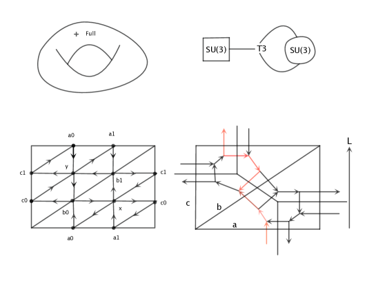
The cluster coordinates (or the quiver) for this theory is constructed as following: one start with a triangulation of once punctured torus, which is the same as the $A_{1}$ case, and the new features are: there are $2$ nodes on each edge, and one extra nodes inside each triangle. The quiver is shown in figure. 11.

It is natural to identify the integral tropical $a$ coordinates as the space of half-BPS line operators. Although this statement is quite powerful, we actually want to know the geometric counterpart which is more useful in many contexts. Namely, we would like to find the geometric representation for each line operator labeled by a tropical $a$ coordinate.

We do have a natural geometric object on the Riemann surface: the closed curve. Since each closed curve represent a weakly coupled gauge group, it is natural to expect that one should get a Wilson loop by wrapping six dimensional surface operator on it, and we would like to know its tropical $a$ coordinates. According to $A_{1}$ theory, the tropical $a$ coordinates can be read from the top component of the canonical map calculated from monodromy; We expect this fact is also true in the higher rank theory, and luckily the way of calculating the monodromy is given in [27]. We are going to use the monodromy calculation to find the tropical $a$ coordinates for each closed curve.

There are three simple nontrivial cycles which we denote as $\mbox{L},\mbox{M},\mbox{ C}$ which can be identified as three duality frames of the corresponding gauge theory, see figure. 9. Let’s consider one duality frame in which the L cycle represents the $\mbox{SU}(3)$ gauge group. A closed curve wrapping around the L cycle should give us a Wilson loop. The monodromy of the closed curves can be similarly found using the following three by three matrices in the same monodromy graph as used for $A_{1}$ theory:

$$\mbox{S}[3]=\begin{pmatrix}0&0&-1\\ 0&1&0\\ -1&0&0\end{pmatrix},~{}~{}\mbox{E}[a,3]=\begin{pmatrix}a_{0}a_{1}&0&0\\ 0&a_{1}&0\\ 0&0&1\end{pmatrix},~{}~{}\mbox{Face}[x,3]=\begin{pmatrix}x&0&0\\ x&x&0\\ x&1+x&1\\ \end{pmatrix}.$$

The above prescription actually gives a PGL(3) matrix and $\mbox{SL}(3)$ canonical map is given by the following formula

$$\mbox{I}(l)=(\mbox{Det}(M))^{-{1\over 3}}\mbox{Tr}(M).$$ (29)

The canonical map of $L$ (we call it as $\mbox{L}_{1}$.) is found using the path in monodromy graph shown in figure. 11; and the monodromy matrix is

$$\mbox{M}=\mbox{E}[a,3]*\mbox{Face}[x,3]*\mbox{E}[b,3]*\mbox{S}[3]^{-1}*\mbox{Face}[y,3]^{-1}*\mbox{S}[3]^{-1};$$ (30)

Using (29), the canonical map for $L_{1}$ is

$$\mbox{I}(\mbox{L}_{1})={1\over{x^{2/3}y^{1/3}a_{0}^{1/3}a_{1}^{2/3}b_{0}^{1/3}b_{1}^{2/3}}}+{{b_{1}^{1/3}}\over{x^{2/3}y^{1/3}a_{0}^{1/3}a_{1}^{2/3}b_{0}^{1/3}}}+\frac{x^{1/3}b_{1}^{1/3}}{y^{1/3}a_{0}^{1/3}a_{1}^{2/3}b_{0}^{1/3}}+\frac{x^{1/3}a_{1}^{1/3}b_{1}^{1/3}}{y^{1/3}a_{0}^{1/3}b_{0}^{1/3}}+$$

$$\frac{x^{1/3}b_{0}^{2/3}b_{1}^{1/3}}{y^{1/3}a_{0}^{1/3}a_{1}^{2/3}}+\frac{x^{1/3}a_{1}^{1/3}b_{0}^{2/3}b_{1}^{1/3}}{y^{1/3}a_{0}^{1/3}}+\frac{x^{1/3}y^{2/3}a_{1}^{1/3}b_{0}^{2/3}b_{1}^{1/3}}{a_{0}^{1/3}}+x^{1/3}y^{2/3}a_{0}^{2/3}a_{1}^{1/3}b_{0}^{2/3}b_{1}^{1/3}.$$ (31)

This is a positive Laurent polynomial with positive integer coefficient, and the exponents of the leading order term should be identified with the tropical $a$ coordinates of $L_{1}$: $(a_{0},a_{1},b_{0},b_{1},c_{0},c_{1},x,y)=({2\over 3},{1\over 3},{2\over 3},{1\over 3},0,0,{1\over 3},{2\over 3})$. We now argue that $L_{1}$ should be identified with the Wilson line in fundamental representation of $\text{SU}(3)$ gauge group by looking at its dual tropical $x$ coordinate:

$$x_{i}=-a_{j}\epsilon_{ij},$$ (32)

and the answer for $L_{1}$ is $(-1,0,1,0,0,0,0,0)$. Now take one of the edge (say $b$ edge) of the triangulation, and there are $2$ dots on it which can be thought of as the Dynkin nodes for the $A_{2}$ group, and our line operator has coordinates $(1,0)$ which is exactly the Dynkin label for fundamental representation of $\mbox{SU}(3)$ group, so it is natural to identify it as the Wilson line in fundamental representation, see figure. 12.

Figure 12: Left: the tropical $a$ coordinates for line operators in cycle $L$ with two different orientations. Right: the tropical $x$ coordinate for $L_{1}$ and $L_{2}$.

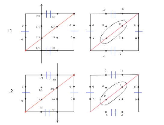
The Wilson loop in anti-fundamental representation is naturally identified with the closed curve with opposite orientation (this is different from $A_{1}$ case in which the orientation does not matter, since the fundamental and anti-fundamental representation of $\mbox{SU}(2)$ group is the same.) The canonical map is calculated using the matrix $M^{-1}$, and the answer is

$$\mbox{I}(\mbox{L}_{2})=\frac{1}{x^{1/3}y^{2/3}a_{0}^{2/3}a_{1}^{1/3}b_{0}^{2/3}b_{1}^{1/3}}+\frac{b_{0}^{1/3}}{x^{1/3}y^{2/3}a_{0}^{2/3}a_{1}^{1/3}b_{1}^{1/3}}+\frac{y^{1/3}b_{0}^{1/3}}{x^{1/3}a_{0}^{2/3}a_{1}^{1/3}b_{1}^{1/3}}+\frac{y^{1/3}a_{0}^{1/3}b_{0}^{1/3}}{x^{1/3}a_{1}^{1/3}b_{1}^{1/3}}+$$

$$\frac{y^{1/3}b_{0}^{1/3}b_{1}^{2/3}}{x^{1/3}a_{0}^{2/3}a_{1}^{1/3}}+\frac{y^{1/3}a_{0}^{1/3}b_{0}^{1/3}b_{1}^{2/3}}{x^{1/3}a_{1}^{1/3}}+\frac{x^{2/3}y^{1/3}a_{0}^{1/3}b_{0}^{1/3}b_{1}^{2/3}}{a_{1}^{1/3}}+x^{2/3}y^{1/3}a_{0}^{1/3}a_{1}^{2/3}b_{0}^{1/3}b_{1}^{2/3}.$$ (33)

Now $a$ coordinates for this line operator is $(a_{0},a_{1},b_{0},b_{1},c_{0},c_{1},x,y)=({1\over 3},{2\over 3},{1\over 3},{2\over 3},0,0,{2\over 3},{1\over 3})$, and the dual $x$ coordinates is $(0,-1,0,1,0,0,0,0)$. The $x$ coordinates on edge $b$ is $(0,1)$ which is exactly the Dynkin label for anti-fundamental representation.

The other irreducible representations for $A_{2}$ group are labeled by two positive integers $(m,n)$. In group representation theory, these other representations can be found by doing the tensor product of $m$ fundamental and $n$ anti-fundamental representation, and expand them in terms of irreducible representation in which $(m,n)$ is the leading order component. Here we use exactly same strategy to find the line operator for the other representations: a line operator with Dynkin label $(m,n)$ can be found as leading component in the OPE of product $\mbox{L}_{1}^{m}\mbox{L}_{2}^{n}$, since the leading order component in the OPE has the tropical $x$ coordinates $(m,n)$ on edge $b$.

The tropical $a$ coordinates of the line operators in representation $(m,n)$ is $ma(\mbox{L}_{1})+na(\mbox{L}_{2})$, and the canonical map can be found by carefully doing the OPE. A very useful fact is that the canonical map for the line operator in $(n,0)$ or $(0,n)$ representations can be found using the monodromy matrix $M^{n}$ and $M^{-n}$ respectively. To find the canonical map of the general representation $(m,n)$, one need to do the OPE expansion of the product $\mbox{L}_{1}^{m}\mbox{L}_{2}^{n}$. Not quite surprisingly, the OPE is closely related to the tensor product of the corresponding representations. More precisely, the support of the the OPE is exactly the same as the corresponding tensor product expansion of the group representation theory, but the coefficient of our OPE is not equal to the multiplicities of the tensor product. Here are some of the examples we found:

$$\mbox{I}(\omega_{1})*\mbox{I}(\omega_{2})=\mbox{I}(\omega_{1}+\omega_{2})+\mbox{I}(0),~{}~{}~{}~{}~{}~{}~{}~{}~{}~{}~{}~{}~{}~{}~{}~{}~{}(3\otimes\bar{3}=8+1)$$

$$\mbox{I}(\omega_{1})*\mbox{I}(\omega_{1})=\mbox{I}(2\omega_{1})+2\mbox{I}(\omega_{2}),~{}~{}~{}~{}~{}~{}~{}~{}~{}~{}~{}~{}~{}~{}~{}~{}~{}~{}~{}(3\otimes 3=6+\bar{3})$$

$$\mbox{I}(\omega_{1}+\omega_{2})*\mbox{I}(\omega_{1})=\mbox{I}(2\omega_{1}+\omega_{2})+2\mbox{I}(2\omega_{2})+2\mbox{I}(\omega_{1}),~{}(8\otimes 3=15+6+3).$$ (34)

Here we use $\omega_{1}$ to denote the line operator in fundamental representation ($\mbox{L}_{1}$) and $\omega_{2}$ to denote the anti-fundamental representation line operator ($\mbox{L}_{2}$), and the trivial line operator (with zero $a$ coordinates) give a number $3$ . Let’s now prove the second OPE in above formula. The canonical map for $(2,0)$ line operator can be found using the monodromy matrix $M^{2}$, and the result is given in the appendix B. Using the canonical map of $\mbox{I}(\omega_{1})$ for $L_{1}$ and $\mbox{I}(\omega_{2})$ for $L_{2}$, one can verify the second OPE in above formula. These wonderful OPE suggests that we got the right answer for the Wilson loops: the Wilson loop is classified by the irreducible representation of the gauge group, and the OPE is related to the tensor product of the corresponding representations. These facts play an important role in the physical approach to Geometric Langlands program in [35].

Let’s now calculate the monodromy around the puncture, and the closed curve is shown in figure. 9. By taking a closed path representing the above closed curve in the monodromy graph, we have the following representation for the monodromy:

$$M_{p}=\mbox{Edge}[e,3].\mbox{Face}[y,3].\mbox{Edge}[a,3].\mbox{Face}[x,3].\mbox{Edge}[b,3].\mbox{Face}[y,3].$$

$$\mbox{Edge}[c,3].\mbox{Face}[x,3].\mbox{Edge}[f,3].\mbox{Face}[y,3].\mbox{Edge}[d,3].\mbox{Face}[x,3]$$ (35)

Notice that we use the different labels for the same edges ($(e=c,a=f,b=d)$), and at the end we should identify the coordinates of the same edge in the following way, say

$$e_{0}=c_{1},e_{1}=c_{0}.$$ (36)

we find a upper triangular matrices whose three diagonal terms (after making the matrix to have determinant one) are

$$\gamma_{11}=a_{0}a_{1}b_{0}b_{1}c_{0}c_{1}xy,~{}~{}\gamma_{22}=xy,~{}~{}~{}\gamma_{33}={1\over a_{0}a_{1}b_{0}b_{1}c_{0}c_{1}x^{2}y^{2}}.$$ (37)

Each diagonal term is the central element in the Poisson structure, and it is natural to regard the first two terms as the independent mass terms:

$$m_{1}=a_{0}a_{1}b_{0}b_{1}c_{0}c_{1}xy,~{}~{}m_{2}=xy.$$ (38)

We take the leading order term as the canonical map for this line operator with positive weights (as motivated by the rule in the $A_{1}$ case):

$$\text{I}(\omega_{1}^{+})=a_{0}a_{1}b_{0}b_{1}c_{0}c_{1}xy.$$ (39)

Here $\omega_{1}^{+}=(1,0)$, and we use this rule following the study of the Wilson line. We can also take the least leading order term as the canonical map for the opposite label:

$$\text{I}(\omega_{1}^{-})={1\over a_{0}a_{1}b_{0}b_{1}c_{0}c_{1}x^{2}y^{2}},$$ (40)

here $\omega_{1}^{-1}=(-1,0)$. Similarly, by calculating the monodromy using the opposite orientation and take the leading order term, we have the canonical map

$$\text{I}(\omega_{2}^{+})=a_{0}a_{1}b_{0}b_{1}c_{0}c_{1}x^{2}y^{2},~{}~{}\text{I}(\omega_{2}^{-})={1\over a_{0}a_{1}b_{0}b_{1}c_{0}c_{1}xy},$$ (41)

with $\omega_{2}^{+}=(0,1),\omega_{2}^{-}=(0,-1)$. The tropical $a$ coordinates can be easily read from the canonical map. More generally, a closed curve around the puncture is labeled by a pair of integers $(m,n)$, and the tropical $a$ coordinates are

$$\text{Trop}((m,n))=\text{Trop}(\omega_{1}^{\text{sgn}(m)})+\text{Trop}(\omega_{2}^{\text{sgn}(n)}).$$ (42)

and the canonical map is just a single monomial in cluster $X$ coordinates with the exponent determined by tropical $a$ coordinates.

3.1.2 The missing line operator

Completely same analysis can be applied to other simple closed curves, say M and C cycles. The conclusion is that the line operators supported on these closed curves are generated by the line operators in the fundamental and anti-fundamental representations, and they are labeled by the irreducible representations of $\text{SU}(3)$ group. In the torus case, we have the generators $\mbox{L}_{1},\mbox{L}_{2},\mbox{M}_{1},\mbox{M}_{2},\mbox{C}_{1},\mbox{C}_{2}$. If we take a duality frame where $L$ cycle represents the weakly coupled gauge group, then $\mbox{M}_{i}$ can be regarded as the ’t Hooft loop operator.

The above story seems to be in parallel with the $A_{1}$ theory. However, something is missing here: first of all, all the line operators we found do not have the charges (tropical $x$ coordinates) under the internal quiver nodes, and secondly there are only six generators for the loop coordinates and one should have at least $8$ to match the total dimension of the cluster coordinates. It is natural that we could not find the extra ones by just looking at the closed curves since they should only carry the charge of the gauge group, and they are not able to probe the internal Coulomb branch operator carried by the $\mbox{T}_{3}$ theory.

Figure 13: The OPE between the Wilson and t’Hooft line operators.

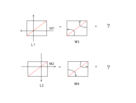
Although a geometric picture for the missing ones is not available yet (we will turn to this later), we should be able to find them by doing the OPE of these usual Wilson and ’t Hooft line operators as they form a closed algebra. Let’s do the OPE for $\mbox{L}_{1}$ and $\mbox{M}_{1}$ (see the appendix for the canonical map of $\mbox{M}_{1}$), see figure. 13. In the OPE, it is natural to expect that the leading order component might be represented by the closed curve $W_{1}$ shown in figure. 13, whose canonical map can be found using monodromy representation. We calculate the canonical map for $W_{1}$ and subtract it from the product of $\text{I}(\text{L}_{1})*\text{I}(\text{M}_{1})$, and indeed we get a positive polynomial which means that it is indeed the top component of the OPE. We are left with a positive Laurent polynomial whose leading order term is (see appendix for the full Laurent polynomial):

$$\mbox{I}(I_{1})=a_{0}^{2/3}a_{1}^{1/3}b_{0}^{1/3}b_{1}^{2/3}c_{0}^{2/3}c_{1}^{1/3}xy+\ldots$$ (43)

This line operator is actually the missing one! The leading order monomial should give the tropical $a$ coordinates for this new line operator. As usual, Let’s find its tropical $x$ coordinates, and the answer is

$$(0,0,0,0,0,0,-1,1),$$ (44)

so it indeed carries the charge under the internal quiver nodes, which strongly suggests that this is the missing line operator we are looking for. Similarly, one can find another internal line operator $I_{2}$ by doing the OPE of $L_{2}$ and $M_{2}$, and after subtracting the canonical map of $W_{4}$, we find the canonical map $\text{I}(\text{I}_{2})$ whose leading order term is

$$\mbox{I}(I_{2})=a_{0}^{1/3}a_{1}^{2/3}b_{0}^{2/3}b_{1}^{1/3}c_{0}^{1/3}c_{1}^{2/3}xy+\ldots\ldots$$ (45)

and it has the tropical $x$ coordinates

$$(0,0,0,0,0,0,1,-1).$$ (46)

Figure 14: The tropical $a$ and tropical $x$ coordinates for $I_{1}$ and $I_{2}$ which are found from OPE between the usual Wilson and ’t Hooft line operators.

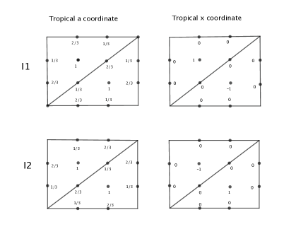
The coordinates of two new line operators are shown in figure. 14. With these two new line operators, we have the following conjecture regarding the generators of the line operator:

Conjecture: The line operators of $A_{2}$ theory on torus with one full puncture are generated by the following eight nontrivial elements:

$$\mbox{L}_{1},\mbox{L}_{2},\mbox{M}_{1},\mbox{M}_{2},\mbox{C}_{1},\mbox{C}_{2},\mbox{I}_{1},\mbox{I}_{2};$$ (47)

By generators, I mean every nontrivial line operator with positive tropical $a$ coordinates can be formed by taking the product of them and take the leading order term in the OPE:

$$l=\prod\mbox{G}_{i}^{n_{i}},$$ (48)

where $G_{i}$ are the above generators. The tropical data for these line operators are listed in table 1.

	Tropical a coordinates	Tropical x coordinates
$L_{1}$	$a_{0}^{2/3}a_{1}^{1/3}b_{0}^{2/3}b_{1}^{1/3}x^{1/3}y^{2/3}$	$(-1,0,1,0,0,0,0,0)$
$L_{2}$	$a_{0}^{1/3}a_{1}^{2/3}b_{0}^{1/3}b_{1}^{2/3}x^{2/3}y^{1/3}$	$(0,-1,0,1,0,0,0,0)$
$M_{1}$	$b_{0}^{2/3}b_{1}^{1/3}c_{0}^{2/3}c_{1}^{1/3}x^{2/3}y^{1/3}$	$(0,0,-1,0,1,0,0,0)$
$M_{2}$	$b_{0}^{1/3}b_{1}^{2/3}c_{0}^{1/3}c_{1}^{2/3}x^{1/3}y^{2/3}$	$(0,0,0,-1,0,1,0,0)$
$C_{1}$	$a_{0}^{2/3}a_{1}^{1/3}c_{0}^{1/3}c_{1}^{2/3}x^{2/3}y^{1/3}$	$(1,0,0,0,0,-1,0,0)$
$C_{2}$	$a_{0}^{1/3}a_{1}^{2/3}c_{0}^{2/3}c_{1}^{1/3}x^{1/3}y^{2/3}$	$(0,1,0,0,-1,0,0,0)$
$I_{1}$	$a_{0}^{2/3}a_{1}^{1/3}b_{0}^{1/3}b_{1}^{2/3}c_{0}^{2/3}c_{1}^{1/3}xy$	$(0,0,0,0,0,0,-1,1)$
$I_{2}$	$a_{0}^{1/3}a_{1}^{2/3}b_{0}^{2/3}b_{1}^{1/3}c_{0}^{1/3}c_{1}^{2/3}xy$	$(0,0,0,0,0,0,1,-1)$

Table 1: The tropical $a$ and $x$ coordinates for eight generators.

3.1.3 Webs and Skein relations

We found these extra line operators by doing OPE, which is purely algebraic as we use the canonical map. One may wonder if there is a geometric structure for them as line operators of 4d $\mathcal{N}=2$ theory should be represented by M2 branes wrapped on one skeleton on Riemann surface. We have already used all the closed curves, so new structure is needed.

It seems the new structures are webs formed by three junctions, i.e. the $\text{I}_{1}$ is formed by connecting two three junctions. Since the extra line operator has nontrivial tropical $x$ coordinate on the internal quiver node, it is natural to put the junction at the internal quiver nodes, and it is useful to label the junction as black if the $x$ coordinate is positive and white if the $x$ coordinate is negative. Based on the tropical $a$ coordinates of the line operator $\text{I}_{1}$ and $\text{I}_{2}$, it is then straightforward to find the $a$ coordinate for the dual triangle of these two junctions, and the result is shown in figure. 15.

Figure 15: Top: the junction and its tropical $a$ coordinates on a dual triangle. Bottom: webs representing $\text{I}_{1}$ and $\text{I}_{2}$.

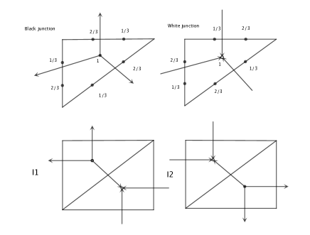
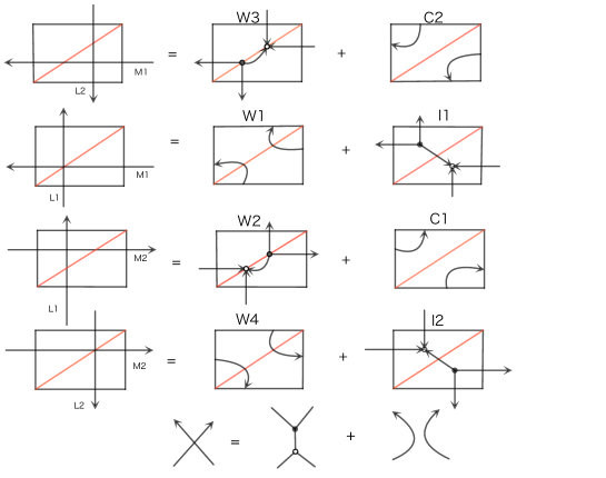
Up to now, the junctions and webs are just a good way of representing the new extra line operator. To make it as something really fundamental, we are going to do OPE for other line operators represented by the closed curves, and the result is shown in figure. 16. $\text{W}_{2}$ (as well as $\text{W}_{3}$) is represented by bipartite webs, and its tropical $a$ coordinates and canonical map can be easily found:

$$\text{I}(\text{W}_{2})=a_{0}^{1/3}a_{1}^{1/3}b_{0}b_{1}c_{0}^{1/3}c_{1}^{2/3}x^{2/3}y^{4/3}+\ldots$$ (49)

Figure 16: Top: The geometric representation for the OPE between the Wilson and ’t Hooft line operators. Bottom: the above OPE can be derived by using this simple Skein relation.

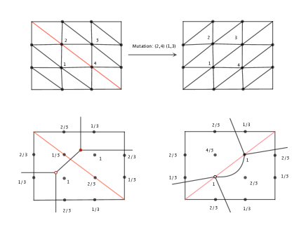
Now a very strong check of the web structure is following: we can use another coordinate system by doing mutation on edge $b$ and write down the tropical $a$ coordinates of $\text{W}_{2}$ using the junction rule indicated in figure. 15, then we mutate back using the mutation sequences $(\mu_{2},\mu_{4}),(\mu_{1},\mu_{3})$, see figure. 17. The $a$ coordinates of $W_{2}$ in original coordinate system can be found using the mutation formula, and remarkably, the answer is the same as given by (49). One can check the transformation of the canonical map and they are actually related by the mutations!

Figure 17: Top: the two quivers of two different triangulations are related by the quiver mutations $(\mu_{2},\mu_{4}),(\mu_{1},\mu_{3})$. Bottom: The transformation of the tropical $a$ coordinates of the $W_{2}$ from one triangulation to another triangulation.

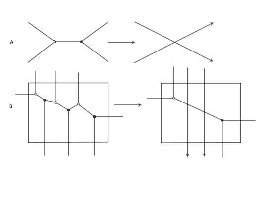
By examining the OPE shown in figure. 16, it is not hard to realize that they can be derived from a local Skein relation shown at the bottom of figure. 16. One might think that the OPE for any line operators can be found using this Skein relation. This is reasonable as one can do following: first draw the closed curves (or webs) for the line operators appearing in the operator product, and use the Skein relation to eliminate all four crossings, etc. However, the above story is not entirely correct, since there is a very crucial thing we want to address: there are trivial crossings between two closed curves, we’d better make sure such configurations are trivial and this would imposed the equivalence condition on the webs. By analyzing the equivalence conditions shown in figure. 18, we get the Skein relation in figure. 18, which we call as bubble reduction and square reduction respectively. So an irreducible web diagram has no two cycles and four cycles, and we conjecture that these are the full Skein relations.

Figure 18: A: The derivation of the bubble reduction and the square reduction. B: The full Skein relations of $A_{2}$ theory.

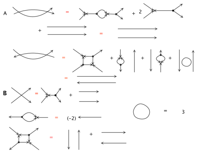
In the following, we will ignore the orientation of the edges in the web diagram, and it is easy to recover the orientations using the rules: the arrow is going from black junction to white junction. Using the above Skein relation, we have the following geometric picture for line operators for $A_{2}$ theory on once punctured torus: all the line operators can be realized as the bipartite webs without two cycles and four cycles on the torus. Let’s look at two simple examples of using Skein relations to find OPE.

Example 1: Let’s consider the OPE of $\mbox{I}_{1}$ and $\mbox{L}_{1}$, and $\mbox{I}_{2}$ and $\mbox{L}_{1}$. Use the Skein relation, one have two line operators in the OPE, see figure. 19.

Figure 19: Upper: OPE of $\mbox{I}(I_{1})*\text{I}(L_{1})$. Middle: OPE of $\text{I}(I_{2})*\text{I}(L_{1})$. Bottom: The OPE of $\mbox{I}(L_{1})*\mbox{I}(L_{2})*\mbox{I}(M_{2})$.

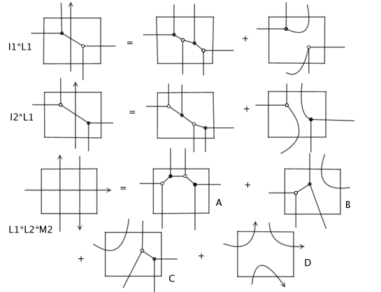
Example 2: Let’s study the OPE of $L_{1}L_{2}M_{2}$ using Skein relation, and the result is shown in figure. 19:

$$\mbox{I}(\text{L}_{1})*\mbox{I}(\text{L}_{2})*\mbox{I}(\text{M}_{2})=\mbox{I}(\text{A})+\mbox{I}(\text{B})+\mbox{I}(\text{C})+3\mbox{I}(\mbox{M}_{2}),$$ (50)

here $A$ is the top component of $\mbox{I}(\text{I}_{2})*\text{I}(\mbox{L}_{1})$, B is the top component of $\mbox{I}(\text{L}_{1})*\mbox{I}(\text{L}_{2})*\mbox{I}(\text{M}_{2})$, C is the top component of $\text{I}(\mbox{L}_{2})*\text{I}(\mbox{C}_{1})$, and D is just $\text{M}_{2}$. Notice that the coefficient $3$ before ${\text{M}}_{2}$ is invisible from using the Skein relation.

The above two examples are in perfect agreement with the calculation using the explicit canonical map. It is amazing that the simple Skein relation reproduces the correct OPE, which strongly suggest that the geometric picture we found for the general line operators are correct!

3.1.4 Construction and reconstruction

The web construction is based on the assumption that the line operators are built from eight generators (the leading component in OPE). The construction of web from $a$ coordinates is rather indirect: we need to first find the combinations of generators and then do OPE. Moreover, we do not know what kind of constraints on $a$ coordinates are needed to have a geometric web representation. So it is important to find a way of constructing webs directly from tropical $a$ coordinate, which is also very useful for dealing with line operators on general Riemann surface. Indeed, we find similar reconstruction procedure as $A_{1}$ case.

Let’s consider a triangle in the triangulation and assume the tropical $a$ coordinates on the quiver nodes as $\tilde{a}_{i}$; We further assume that the dual $x$ coordinates of the internal quiver nodes to be positive. We multiple each tropical coordinates by 3, i.e. $a_{0}=3\tilde{a}_{0}$, such that all the coordinates are integers now.

The idea of reconstruction is to construct set of non-intersecting curves (junction) inside the triangle such that they give the desired $a$ coordinates. There are actually seven kinds of curves: two curves around each vertex and one junction (only one type of junctions is allowed as we will see shortly). So let’s assume there are $n_{1}$ ($n_{2}$) anti-clockwise (clockwise) curves around vertex $A$, and we use the similar notation for other two vertices; finally let’s assume there are $J$ black junctions inside the triangle. Summing up the contribution of each curve to the tropical $a$ coordinate on seven quiver nodes, we have the following equations:

$$2n_{1}+n_{2}+m_{1}+2m_{2}+2J=a_{0},~{}~{}n_{1}+2n_{2}+2m_{1}+m_{2}+J=a_{1},$$

$$2m_{1}+m_{2}+l_{1}+2l_{2}+2J=b_{0},~{}~{}m_{1}+2m_{2}+2l_{1}+l_{2}+J=b_{1},$$

$$2l_{1}+l_{2}+n_{1}+2n_{2}+2J=c_{0},~{}~{}~{}~{}~{}l_{1}+2l_{2}+2n_{1}+n_{2}+J=c_{1},$$

$$n_{1}+2n_{2}+m_{1}+2m_{2}+l_{1}+2l_{2}+3J=x_{0}.$$ (51)

The solution is uniquely fixed by the tropical $a$ coordinates:

$$n_{1}=\frac{1}{3}(a_{0}+c_{1}-x_{0}),~{}n_{2}=\frac{1}{3}(-a_{0}+a_{1}-b_{0}+x_{0}),~{}$$

$$m_{1}=\frac{1}{3}(a_{1}+b_{0}-x_{0}),~{}m_{2}=\frac{1}{3}(-b_{0}+b_{1}-c_{0}+x_{0}),$$

$$l_{1}=\frac{1}{3}(b_{1}+c_{0}-x_{0}),~{}~{}l_{2}=\frac{1}{3}(-a_{0}-c_{0}+c_{1}+x_{0}),~{}J={1\over 3}({a_{0}-a_{1}+b_{0}-b_{1}+c_{0}-c_{1}}).$$ (52)

Interestingly, $J$ is the tropical $x$ coordinates of the internal quiver nodes and therefore is a positive integer, which should be the case since only the junction can carry the tropical $x$ charge of the internal quiver nodes. Notice that the number of marked points on one edge $AB$ is equal to

$$n_{1}+n_{2}+J+m_{1}+m_{2}={1\over 3}(a_{0}+a_{1})=\tilde{a}_{1}+\tilde{a}_{0},$$ (53)

which actually only depends on the coordinate on the edge $AB$. Moreover, the number of curves coming into $AB$ are $n_{1}+m_{2}+J=2\tilde{a}_{0}-\tilde{a}_{1}$, and the number of outgoing curves is $n_{2}+m_{1}=2\tilde{a}_{1}-\tilde{a}_{0}$, which also only depend on the coordinates on the edge. To make all these numbers to be positive integer, we need to put the following constraints on the tropical $a$ coordinates on the edge:

$$\tilde{a}_{0}+\tilde{a}_{1}\in z$$

$$\tilde{a}_{0}\leq 2\tilde{a}_{1},~{}~{}\tilde{a}_{1}\leq 2\tilde{a}_{0}.$$ (54)

Moreover, we need the following constraints:

$$\tilde{\alpha}+\tilde{\beta}+2\tilde{\gamma}\in z,~{}\tilde{\gamma}\leq\tilde{\alpha}+\tilde{\beta}$$ (55)

where $\tilde{\gamma}$ is the coordinate on internal quiver node, and $\tilde{\alpha},\tilde{\beta}$ are quiver nodes in the same quiver triangle as $\tilde{\gamma}$, say $(\tilde{\alpha},\tilde{\beta},\tilde{\gamma})=(a_{0},c_{1},x_{0})$ in figure. 20. One can easily see that above three constraints would ensure the solutions in (52) are all positive integers! Similarly, if the tropical $x$ coordinate of the internal quiver node is negative, we have the solution:

$$n_{1}=\frac{1}{3}(a_{0}+c_{1}-x_{0}),~{}n_{2}=\frac{1}{3}(c_{0}-c_{1}-b_{1}+x_{0}),~{}$$

$$m_{1}=\frac{1}{3}(a_{1}+b_{0}-x_{0}),~{}m_{2}=\frac{1}{3}(a_{0}-a_{1}-c_{1}+x_{0}),$$

$$l_{1}=\frac{1}{3}(b_{1}+c_{0}-x_{0}),~{}~{}l_{2}=\frac{1}{3}(-a_{1}+b_{0}-b_{1}+x_{0}),~{}J={1\over 3}({-a_{0}+a_{1}-b_{0}+b_{1}-c_{0}+c_{1}}),$$ (56)

and $J$ is equal to the minus of the internal tropical $x$ coordinate and therefore is positive. The constraints are the same as the above case.

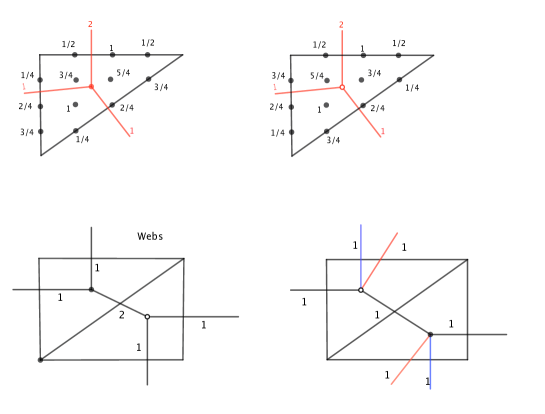
Example: Let’s look at an example, the coordinates on the triangle are

$$(a_{0},a_{1},b_{0},b_{1},c_{0},c_{1},x_{0})=(5,4,1,2,3,6,5),$$ (57)

see figure. 20, so the marked points on each edge are $(AB,BC,CA)=(3,1,3)$. Since the tropical $x$ coordinates of internal quiver node is negative, we need to use solution (56). Substitute the coordinates into the formula, we have

$$(n_{1},n_{2},m_{1},m_{2},l_{1},l_{2},J)=(2,0,0,0,0,0,1),$$ (58)

so there is one white junction inside triangle and two clockwise curves around vertex $A$.

Figure 20: Top: construct curves from tropical $a$ coordinates on a triangle. Bottom: construct webs on a torus from tropical $a$ coordinates.

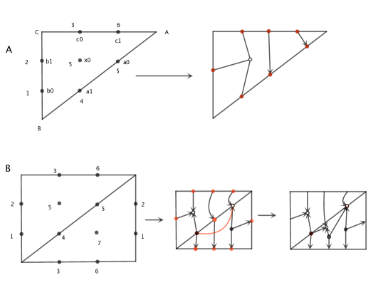
Now given a set of $a$ coordinates, we do the above reconstruction for each triangle, then we can form a set of closed non-intersecting webs and closed curves on Riemann surface. However, there are two complications we need to address: firstly the web has crossings if there are more than one three junctions inside the triangle; and secondly the marked points on the edge can be source (two arrows come out) or sinks (two arrows coming in). The first complication is easy to address: one replace each crossing by a piece with two junctions using the Skein relation, see an example in figure. 21. One always produce an irreducible sub web in this step as all the closed surfaces are hexagons.

The second complication is a little bit difficult to deal with. First, let’s color a marked points as black (white) if it is source (sink), and it is not hard to observe the following fact: the number of black and white vertices are the same. We can then connect the white and black vertices in pairs and produce a lot of crossings. The resolution of the crossings are different based on the origin of two crossing lines:

• If the two lines coming from the vertices with different color, we keep the second term (two curves) in the Skein relation.

• If the two lines coming from the vertices with same color, we keep the first term (two junctions) in the Skein relation.

• If one of two crossing line is a ordinary line connecting two internal junctions, we keep the second term in the Skein relation; otherwise, we keep the second term.

Using the above rules, we can produce an irreducible bipartite web around the edges. However, we do not know whether this procedure will produce an irreducible web in gluing the triangles together. This is true for all the examples we check, and it would be nice to have a proof though.

Figure 21: Top: resolve the crossing of the three junctions inside the triangle. Bottom: resolve the crossing around the edges.

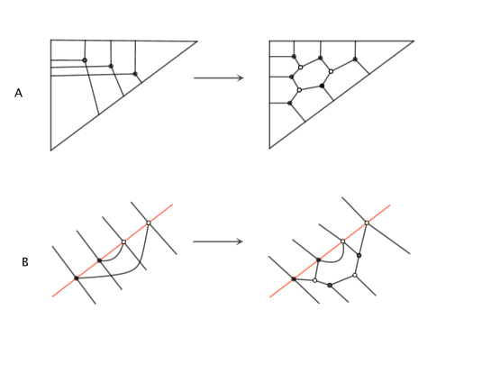
In the above consideration, we start with a set of tropical $a$ coordinates and then construct an irreducible web. On the other hand, if we start with a web, we would like to find its tropical $a$ coordinates. This can be found by doing reverse Skein relation, namely one replace two junctions with a four crossings, see figure. 22. The above procedure stops if four legs of the two junctions are on the boundary. At the end, we are left with the basic building blocks: closed curves and $\text{I}_{1},\text{I}_{2}$. By taking a triangulation, one know the cluster coordinates for each individual component, and the coordinates are just the sum of that of components.

For example, according to above method, the web diagram in figure. 22 is reduced to three generators $(\text{L}_{2},\text{L}_{2},\text{I}_{2})$. So the original web is the top component of the product $\mbox{I}_{2}*\mbox{L}_{2}*\mbox{L}_{2}$ and its $a$ coordinates are equal to $\text{Trop}(\mbox{I}_{2})+\text{Trop}(\mbox{L}_{2})+\text{Trop}(\mbox{L}_{2})$, which actually equal to the $a$ coordinates we used in last example. The result is in perfect agreement with the one shown in figure. 20, in which we construct the same web from same tropical $a$ coordinates. Moreover, once the set of generators are found, one can find the canonical map of initial web by doing OPE.

Figure 22: A: replace two junctions with the crossing. B: We replace a web with a set of generators from which the $a$ coordinates of the initial web is read.

Now we have established a one-to-one correspondence between the constrained tropical $a$ coordinates (see [54, [55]) and irreducible bipartite webs. This description is exactly the same as the $A_{1}$ case.

It is worth to remark that bipartite network on bordered Riemann surface appears in many different physical contexts: 4d $\mathcal{N}=1$ superconformal field theory [36, 37], BPS quiver for 4d $\mathcal{N}=2$ theory [32, 28], and scattering amplitude of $\mathcal{N}=4$ SYM [38]. The web diagram we found here is of a different kind; the equivalence conditions are different: we do not have square move, but we have bubble and square reduction.

3.1.5 A further check: Poisson brackets

Let’s now verify that the basic line operators (eight generators) are indeed the coordinates for the cluster variety associated with the moduli space of the local system on a torus with one full puncture. The most convincing check is to find the explicit Poisson brackets of these line operators, and show that there are indeed three commuting Hamiltonian as suggested by the underlying Hitchin integrable system.

The Poisson bracket of line operators can be easily found due to the remarkably simple Poisson structure for the cluster $X$ coordinates, which takes the following simple form:

$$[X_{i},X_{j}]=\epsilon_{ij}X_{i}X_{j},$$ (59)

here $\epsilon_{ij}$ is the antisymmetric tensor read from the quiver. It is very easy to calculate the Poisson bracket for two loop operators using the canonical map which is just a positive Laurent polynomial in $X_{i}$. First, for two monomials $A$ and $B$, the Poisson bracket is simply

$$[A,B]=(\sum_{i}a_{A}^{i}x_{B}^{i})A*B,$$ (60)

here $a_{A}$ is the tropical $a$ coordinates for the monomial $A$, and $B$ is the tropical $x$ coordinates for $B$. Using the above noted relation, we could easily calculate the Poisson structure between the eight generators using the explicit canonical map (See appendix B for their canonical maps.), and the Poisson brackets are indeed closed:

$$[L_{1},M_{1}]=-{2\over 3}L_{1}M_{1}+I_{1},~{}~{}~{}~{}[L_{1},M_{2}]=-{1\over 3}L_{1}M_{2}+C_{1}$$

$$[L_{1},C_{1}]={2\over 3}L_{1}C_{1}-I_{2},~{}~{}~{}~{}~{}~{}~{}~{}[L_{1},C_{2}]={1\over 3}L_{1}C_{2}-M_{1}$$

$$[L_{1},I_{1}]={1\over 3}L_{1}I_{1}-L_{2}M_{1}+C_{2},~{}~{}~{}~{}[L_{1},I_{2}]=-{1\over 3}L_{1}I_{2}+L_{2}C_{1}-M_{2}$$ (61)

$$[L_{2},M_{2}]=-{2\over 3}L_{2}M_{2}+I_{2},~{}~{}~{}~{}[L_{2},M_{1}]=-{1\over 3}L_{2}M_{1}+C_{2}$$

$$[L_{2},C_{2}]={2\over 3}L_{2}C_{2}-I_{1},~{}~{}~{}~{}~{}~{}~{}~{}[L_{2},C_{1}]={1\over 3}L_{2}C_{1}-M_{2}$$

$$[L_{2},I_{2}]={1\over 3}L_{2}I_{2}-L_{1}M_{2}+C_{1},~{}~{}~{}~{}[L_{2},I_{1}]=-{1\over 3}L_{2}I_{1}+L_{1}C_{2}-M_{1}$$ (62)

The other brackets are very similar

$$[M_{1},C_{1}]=-{1\over 3}M_{1}C_{1}+L_{1},~{}~{}~{}~{}~{}[M_{1},C_{2}]=-{2\over 3}M_{2}C_{2}+I_{2}$$

$$[M_{1},I_{1}]=-{1\over 3}M_{1}L_{1}+L_{1}M_{2}-C_{1},~{}~{}~{}~{}[M_{1},I_{2}]={1\over 3}M_{1}I_{2}-M_{2}C_{2}+L_{2}$$

$$[M_{2},C_{1}]=-{2\over 3}M_{2}C_{1}+I_{2},~{}~{}~{}[M_{2},C_{2}]=-{1\over 3}M_{2}C_{2}+L_{2}$$

$$[M_{2},I_{1}]={1\over 3}M_{2}I_{1}-M_{1}C_{1}+L_{1},~{}~{}[M_{2},I_{2}]=-{1\over 3}M_{2}I_{2}+L_{2}M_{1}-C_{2}$$ (63)

and

$$[C_{1},I_{1}]=-{1\over 3}C_{1}I_{1}+C_{2}M_{2}-L_{2},~{}~{}[C_{1},I_{2}]={1\over 3}C_{1}I_{2}-C_{2}L_{1}+M_{1}$$

$$[C_{2},I_{1}]={1\over 3}C_{2}I_{1}-C_{1}L_{2}+M_{1},~{}~{}~{}~{}~{}[C_{2},I_{2}]=-{1\over 3}C_{2}I_{2}+C_{1}M_{1}-L_{1}$$

$$[I_{1},I_{2}]=L_{2}M_{1}C_{1}-L_{1}M_{2}C_{2}.$$ (64)

There are actually two central elements which could be found from the above Poisson structure. One of them is

$$I_{1}I_{2}-L_{1}M_{2}C_{2}-L_{2}M_{1}C_{1}+C_{1}C_{2}+M_{1}M_{2}+L_{1}L_{2}$$

$$=3+m_{1}+m_{2}+m_{1}m_{2}+{1\over m_{1}}+{1\over m_{2}}+{1\over m_{1}m_{2}},$$ (65)

and $m_{1},m_{2}$ is expressed as the Fock-Goncharov coordinates as

$$m_{1}=xy,~{}~{}~{}m_{2}=a_{0}a_{1}b_{0}b_{1}c_{0}c_{1}xy.$$ (66)

Since $m_{1}$ and $m_{2}$ are the central elements of the Poisson bracket, and the above polynomial is also a central element. The other central element is much more complicated:

$$L_{1}L_{2}M_{1}M_{2}C_{1}C_{2}+L_{1}^{3}+L_{2}^{3}+M_{1}^{3}+M_{2}^{3}+C_{1}^{3}+C_{2}^{3}-I_{1}^{3}-I_{2}^{3}+3I_{1}C_{1}L_{1}$$

$$+3I_{2}C_{2}L_{2}+3I_{1}L_{2}M_{2}+3I_{2}L_{1}M_{1}+3I_{1}M_{2}C_{2}+3I_{2}M_{1}C_{1}-3L_{1}M_{2}C_{2}-3L_{2}M_{1}C_{1}$$

$$-2C_{2}^{2}L_{2}M_{1}-2C_{1}^{2}L_{1}M_{2}-2C_{1}L_{1}^{2}M_{1}-2C_{2}L_{1}M_{1}^{2}-2C_{2}L_{2}^{2}M_{2}-2C_{1}L_{2}M_{2}^{2}$$

$$-C_{2}^{2}I_{1}L_{1}-C_{2}^{2}I_{2}M_{2}-C_{1}^{2}I_{2}L_{2}-C_{1}^{2}I_{1}M_{1}-L_{1}^{2}C_{2}I_{2}-L_{1}^{2}I_{1}M_{2}-L_{2}^{2}C_{1}I_{1}-$$

$$L_{2}^{2}I_{2}M_{1}-M_{1}^{2}C_{1}I_{2}-M_{1}^{2}I_{1}L_{2}-M_{2}^{2}C_{2}I_{1}-M_{2}^{2}I_{2}L_{1}+I_{1}^{2}L_{1}M_{1}+C_{1}I_{1}^{2}M_{2}+C_{2}I_{1}^{2}L_{2}+C_{2}I_{2}^{2}M_{1}$$

$$+I_{2}^{2}L_{2}M_{2}+C_{1}I_{2}^{2}L_{1}+C_{1}C_{2}L_{1}L_{2}+C_{1}C_{2}M_{1}M_{2}+L_{1}L_{2}M_{1}M_{2}+I_{1}I_{2}M_{1}M_{2}+I_{1}I_{2}L_{1}L_{2}+C_{1}C_{2}I_{1}I_{2}$$

$$C_{2}L_{2}^{2}M_{1}^{2}+C_{1}L_{1}^{2}M_{2}^{2}+C_{1}^{2}L_{2}^{2}M_{2}+C_{2}^{2}L_{1}^{2}M_{1}+C_{2}^{2}L_{2}M_{2}^{2}+C_{1}^{2}L_{1}M_{1}^{2}$$

$$-C_{1}C_{2}I_{2}L_{1}M_{1}-C_{1}C_{2}I_{1}L_{2}M_{2}-C_{1}I_{2}L_{1}L_{2}M_{2}-C_{1}I_{1}L_{1}M_{1}M_{2}-C_{2}I_{2}L_{2}M_{1}M_{2}-L_{1}L_{2}C_{2}I_{1}M_{1}$$

$$=12+\frac{6}{xy}+6xy+\frac{1}{x^{3}y^{3}a_{0}^{2}a_{1}^{2}b_{0}^{2}b_{1}^{2}c_{0}^{2}c_{1}^{2}}+\frac{1}{a_{0}a_{1}b_{0}b_{1}c_{0}c_{1}}+\frac{1}{x^{3}y^{3}a_{0}a_{1}b_{0}b_{1}c_{0}c_{1}}+\frac{6}{x^{2}y^{2}a_{0}a_{1}b_{0}b_{1}c_{0}c_{1}}+$$

$$\frac{6}{xya_{0}a_{1}b_{0}b_{1}c_{0}c_{1}}+a_{0}a_{1}b_{0}b_{1}c_{0}c_{1}+6xya_{0}a_{1}b_{0}b_{1}c_{0}c_{1}+6x^{2}y^{2}a_{0}a_{1}b_{0}b_{1}c_{0}c_{1}$$

$$+x^{3}y^{3}a_{0}a_{1}b_{0}b_{1}c_{0}c_{1}+x^{3}y^{3}a_{0}^{2}a_{1}^{2}b_{0}^{2}b_{1}^{2}c_{0}^{2}c_{1}^{2}=$$

$$12+6({1\over m_{1}}+m_{1}+{1\over m_{2}}+m_{2}+{m_{1}\over m_{2}}+{m_{2}\over m_{1}})+{1\over m_{2}^{2}m_{1}}+m_{2}^{2}m_{1}+{1\over m_{2}^{2}m_{1}}+{m_{1}\over m_{2}}+m_{1}^{2}m_{2}.$$ (67)

Although the above formula seems to be very complicated, it is actually very easy to find using the canonical map. The key observation is the following: the central element is represented by the closed curves around the puncture and their dual $x$ coordinate is zero! So if we can find the combinations of the simple generators such that their tropical $x$ coordinates are vanishing, then its leading component is definitely a central element! We actually have only two independent choices $I_{1}I_{2}$ and $L_{1}L_{2}M_{1}M_{2}C_{1}C_{2}$, which give the leading term in the above central element. The full expression is found by doing OPE of $\text{I}(I_{1})*\text{I}(I_{2})$ and the OPE has the following form:

$$\text{I}(I_{1})*\text{I}(I_{2})=\text{Central~{}terms}+\sum\prod_{i}G_{i}^{n_{i}};$$ (68)

and the polynomial $(I_{1}*I_{2}-\sum\prod_{i}G_{i}^{n_{i}})$ is the central element. We also find the following three commuting Hamiltonians:

$$H_{1}=L_{1}*L_{2},$$

$$H_{2}=L_{1}^{3}+L_{2}^{3},$$

$$H_{3}=L_{1}^{2}C_{1}M_{1}+L_{2}^{2}C_{2}M_{2}+I_{1}I_{2}+M_{1}M_{2}+C_{1}C_{2}+L_{1}L_{2}$$

$$-(I_{2}C_{2}L_{2}+M_{2}L_{2}I_{1}+I_{1}C_{1}L_{1}+M_{1}L_{1}I_{2}).$$ (69)

In fact, one can choose any linear combinations of $L_{1}$ and $L_{2}$ since they both commute with $H_{3}$. The Poisson bracket for eight coordinates $L_{i},M_{i},C_{i},I_{i}$ are closed, so they are good coordinates for the Poisson manifold. We have found two central elements and three commuting Hamiltonians, therefore it is an integrable system as it should be. The action variable can be found such that the symplectic structure has the canonical form

$$\omega=\sum_{i}dH_{i}\wedge d\theta_{i}.$$ (70)

The detailed form for $\theta$ coordinates will be presented elsewhere. These explicit calculations provide very strong evidence that we have the right answer for 4d $\mathcal{N}=2$ line operators!

3.2 General N

3.2.1 Basic building blocks

Let’s consider line operators of 4d theory defined using general $A_{N-1}$ $(2,0)$ theory on once punctured torus. The $\mathcal{N}=2$ theory in one duality frame is described by gauging the diagonal of two $\mbox{SU}(N)$ flavor symmetries of $\mbox{T}_{N}$ theory. The $\mbox{T}_{N}$ theory has $(N-1)(N-2)\over 2$ Coulomb branch operators, and the $\text{SU}(N)$ gauge group has $(N-1)$ Coulomb branch operators; There are also $(N-1)$ mass parameters carried by the full puncture, so the rank of the charge lattice is

$$R=(N-1)(N-2)+2(N-1)+(N-1)=N^{2}-1.$$ (71)

The cluster coordinates are found by Fock and Goncharov: first take an ideal triangulation of the once punctured torus and then put $(N-1)(N-2)\over 2$ more quiver nodes inside each triangle. The total number of quiver nodes is equal to the rank of the charge lattice of 4d theory, for more details, see [32, 28].

The ordinary Wilson lines are represented by the closed curves on the Riemann surface. The tropical $a$ coordinates for Wilson loop in fundamental representation $\omega_{1}$ and anti-fundamental representation $\omega_{N-1}$ are found by calculating the monodromy M and $\text{M}^{-1}$ around the simple closed curve using the similar combinatorial method as $A_{1}$ and $A_{2}$ case, say appendix A for more details.

Once the canonical map (the positive Laurent polynomial) is found, its tropical $a$ coordinates are read from the leading order term. There are other fundamental representations whose tropical $a$ coordinates and the canonical map can be found by doing the OPEs of the two basic fundamentals. A useful fact is that the canonical map of the representation $(n,0,\ldots,0)$ and $(0,\ldots,0,n)$ can be found by taking the trace of the monodromy matrices $\text{M}^{n}$ and $\text{M}^{-n}$. For example, we can do the product $\text{I}(\omega_{1})*\text{I}(\omega_{1})$, where $\omega_{1}$ is the fundamental representation, and the same tensor product from the group theory tells us that the OPE has two components $(2,0,0\ldots,0)$ and $(0,1,\ldots,0)$, since we know the canonical map for representation $(2,0,0\ldots,0)$, we can easily find the canonical map for the second fundamental representation and its $a$ coordinates. Using OPE, one can find the tropical $a$ coordinates for all fundamental representation $\omega_{i}$.

Figure 23: The tropical $a$ coordinates for the Wilson line in the $i$th fundamental representation: the quiver nodes in each straight line have the same indicated tropical $a$ coordinates.

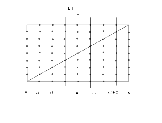
Instead of using the OPE to find the tropical $a$ coordinates of $\omega_{i}$, one can actually find the answer using the following requirement: the tropical $x$ coordinates on the $i$th quiver node of $a$ and $b$ edge should be $\pm 1$ while all the other $x$ coordinates are vanishing. The answer is:

$$a_{1}={N-i\over N},a_{2}={2(N-i)\over N},\ldots,a_{i}={i(N-i)\over N},\ldots,a_{N-2}={2i\over N},a_{N-1}={i\over N};$$ (72)

namely, the $a$ coordinates take the maximal value at the $i$th line, and decreases along the left and right direction, see figure. 23. So it is natural to represent such line operators as the closed curve going through the ith line in the quiver diagram.

After finding the tropical $a$ coordinates and the canonical map of the fundamental representations, one can find all other representations by doing the OPE, which has the same support as the tensor product of the group theory. The conclusion is: the Wilson line is classified by the irreducible representation of $\text{SU}(N)$ group.

Again, these ordinary Wilson operators around three one cycles are not enough. The extra line operators can be found by doing the OPE between the Wilson line operators $L_{i}$ and ’t Hooft operators $M_{j}$ , and the extra line operator is found as the sub-leading component in the OPE. There are a total of $(N-1)^{2}$ pairs and the $N-1$ pairs ($L_{i}$ and $M_{N-i}$) which will give the line operators in the C cycle, therefore we have $(N-1)(N-2)$ number of extra line operators which exactly match the number of internal quiver nodes inside two triangles. The canonical map of the extra line operator can be found using the Poisson bracket: One calculate the Poisson bracket of $L_{i}$ and $M_{j}$, and the result would have two parts with different coefficients, and these two parts are the canonical map of two line operators in the OPE.

These extra line operators can be represented geometrically using three junctions. By doing the explicit OPE, we find that there are ${(N-1)(N-2)\over 2}$ type of three junctions which labeled by three positive integers satisfying the following conditions:

$$i+j+k=N.$$ (73)

It is easy to see that the total number of solutions are ${(N-1)(N-2)\over 2}$ which equals to the number of internal quiver nodes inside one triangle. For each solution, there are two types of junctions such that the internal quiver nodes has positive (negative) tropical $x$ coordinate.

For the black junction, the arrows are coming out of the junction for all three legs while the arrows are coming into the junction for white junction, and we need to label the junction by $(i,j,k)$, see figure. 24. In the $N=3$ case, there is only one solution for the above equation, therefore there is no need to specify the label for the legs.

Figure 24: Top: the black and white junction with labels $(i,j,k)$, and the meaning of the label is that the tropical $a$ coordinates is maximal on $i$th node counting in clockwise direction for the black junction, and anti-clockwise direction for white junction. Bottom: the rule of finding the tropical $a$ coordinates from using fundamental representation $\omega_{i}$ and $\omega_{j}$: first sum up the $a$ coordinates of $\omega_{i}$ and $\omega_{j}$ and then subtract $2$ for the green nodes, and $1$ on the red nodes.

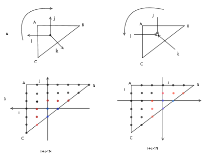
Let’s now describe the tropical $a$ coordinates on the quiver nodes of the dual triangle of black and white junctions. Again, the rules are found by looking the OPE of the line operators $L_{j}$ and $M_{i}$. For the black junction, the tropical $a$ coordinates of the internal quiver nodes and the third edge are found as following: first let’s draw two lines $L_{j}$ and and $M_{i}$ in the $i$ and $j$ directions of the three junction; secondly, sum up the tropical $a$ coordinates of the line operators $L_{j}$ and $M_{i}$, finally we need to subtract appropriate integer number for the above tropical $a$ on edge $BC$ such that they are the tropical coordinates of the $k$th fundamental representation (this can always be achieved), moreover, one need to subtract integer numbers from tropical $a$ coordinates of some of the internal quiver nodes, the pattern is summarized in figure. 24. Similarly procedure can be done for the white junction.

The dual tropical $x$ coordinate of the junction would have non-vanishing value on only one internal quiver node. Using the above explicitly described tropical $a$ coordinate, we find the position of the quiver node which the junction lives:

$$\begin{cases}&(a,b,c)=(i,j,k),~{}~{}\text{Black junction}\\ &(a,b,c)=(j,k,i),~{}~{}\text{White junction}.\end{cases}$$ (74)

One new feature is that one can have $M$ junction with labels $i_{1},i_{2},\ldots,i_{M}$ such that

$$i_{1}+i_{2}+\ldots+i_{M}=N;$$ (75)

Such general junction can be formed using a sequence of three junctions by un-merging junction into a sequence of three junctions, so there is essentially nothing new.

We oriented all the Wilson line in the same orientations as the first fundamental representation. For the following purpose, it is natural to choose a different rule for the orientation: the $i$th fundamental representation with $1\leq i<{N\over 2}$ has the same orientation as $\omega_{1}$, otherwise it is oriented in the orientation as $\omega_{N-1}$ and the label is changed to $i^{{}^{\prime}}=N-i$. If $i={N\over 2}$ and is an integer, the corresponding representation is real, and we do not assign any orientation to it. With this convention, all the curves have the label with value less or equal than ${N\over 2}$.

Accordingly, one need to change the orientation and the label for three junctions. The rules are actually very simple: because of the constraint $i+j+k=N$, there is at most one edge with label bigger than $N/2$, and if there is such type of edge, one simply change its orientation and change the label to $N-i$. The two representations have different advantages: the first one is good for constructing the complicated webs using the basic junctions, while the second one is good for the Skein relations we are going to study in the following. It is not hard to transform between these two representations. The basic junctions and its tropical $a$ coordinates for $A_{3}$ theory are given in figure. 25, and we build some webs using the basic junctions in figure. 25.

Figure 25: Top: the basic junctions and its dual tropical $a$ coordinates of $A_{3}$ theory. Bottom: some webs of $A_{3}$ theory.

3.2.2 Skein relations

After describing the basic geometric building blocks for the webs, it is straightforward to develop the Skein relations and have a geometric representation for the OPE. In the mean time, any 4d line operator would be represented by the bipartite webs on the corresponding Riemann surface. For the purpose of Skein relations, it is useful to use second labeling for the three junctions, i.e. all the labels have value less than or equal ${N\over 2}$. Two legs of two different junctions with same label and opposite orientations (including the legs without orientation) can be connected, and one can have multi-junction, which is different from the $\text{SU}(3)$ case in which one can only have the three junction.

Figure 26: Skein relations for general higher rank theory, here we assume $i+j<{N\over 2}$ to draw the orientation for the new generated legs.

Figure 27: The Skein relation for resolving the crossing for $\text{SU}(4)$ theory.

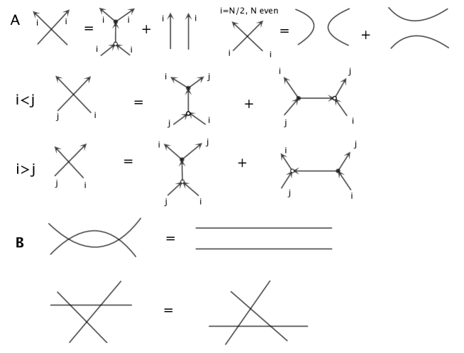
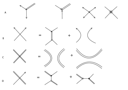
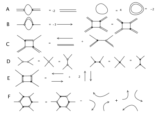
The Skein relation between two oriented lines can be easily found by doing the OPE between the ordinary Wilson and t’ Hoof operators in various fundamental representations, and the result is summarized in figure.26. There are more Skein relations involving bubbles, squares, and hexagons which are derived from obvious equivalence relations shown in figure.26. A full Skein relations can be written down for $N=4$ case, since there is actually just one type of junction with three legs labeled by $(1,1,2)$. Instead of labeling the edge with numbers, we use double line to represent the legs with label $2$, and there is no need to specify its orientation since the corresponding representation is real. The two types of three junction are shown in figure. 27A, moreover, we have the four junctions which can be formed by combining the three junctions. The Skein relation for resolving the cross of two lines are shown in figure. 28. The details for the general cases are tedious and we leave it to the interested reader.

Again, one can start with arbitrary tropical $a$ coordinates and construct the webs using a similar reconstruction procedure as the one developed for $A_{2}$ theory. One the other hand, one can start with an irreducible webs and find its tropical $a$ coordinates. Our conjecture is that there is a one-to-one correspondence between the geometric and the algebraic description.

Figure 28: The full Skein relations of $\text{SU}(4)$ theory.

4 General bordered Riemann surface

We discovered the basic ingredients such as line segments and three junctions with their coordinates on the dual triangle from the study of line operators on once punctured torus; we also find Skein relations which are very powerful in finding the OPE. The above elements are completely local and do not depend on the global structure of Riemann surface, therefore they should still be valid on any bordered Riemann surface. We have the following conjecture: 4d line operator is built as an irreducible bipartite web on the Riemann surface, and the OPE can be found using Skein relations, etc. Other things like tropical $a$ coordinates and canonical map are very similar. In the following, we are going to study the webs on several interesting bordered Riemann surfaces, and we use $A_{2}$ theory as the main examples (the other cases are very similar).

4.1 $T_{N}$ theory

$T_{N}$ theory is defined by a sphere with three full punctures, and is a strongly coupled SCFT with $\text{SU(N)}^{3}$ flavor symmetry. There is no nontrivial closed cycle for three punctured sphere, which means that there is no weakly coupled gauge theory description, so there is no ordinary Wilson line.

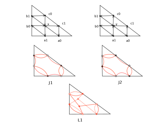
There are ${(N-1)(N-2)\over 2}$ Coulomb branch parameters and we should have non-trivial line operators represented by the webs using three junctions. The simplest one is built by two junctions: for each black junction with $i+j+k=N$, one naturally has a white junction on the back of the sphere to form a closed web, see figure. 29A. There are a total of $(N-1)(N-2)$ of such webs as one can easily count. In figure. 29A, we show the simplest web operators built from two junctions for $T_{3}$ theory, which are denoted as $A_{1}$ and $A_{2}$. They can also be represented by the web on a plane graph in which the puncture is represented by a hole without any marked point, see figure. 29A.

Figure 29: A: the simplest webs on three punctured sphere. B: the OPE between above two webs are found using Skein relations, and there are two non-trivial webs in the OPE.

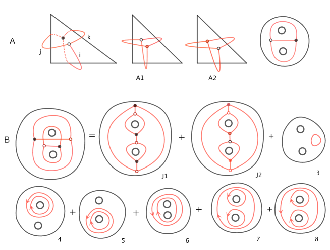
In figure. 29B, we use Skein relations to derive the OPE of $A_{1}$ and $A_{2}$, and two nontrivial line operators appear which are denoted as $J_{1}$ and $J_{2}$. We can further do OPE between $A_{i}$ and $J_{i}$, and find four more new line operators formed by eight three junctions, etc. Therefore, our conjecture is that the space of line operator is the same as the space of irreducible bipartite webs on three punctured sphere.

Given a triangulation and the cluster coordinates [32], the tropical $a$ coordinates of the web can be found using the basic rule for three junction. The canonical map for them is nontrivial since here we can not use the monodromy of the ordinary Wilson line operator and OPE. We do know the leading order term which can be read from the tropical $a$ coordinates of the junctions, and the sub-leading order term is derived using the OPE:

$$I(A_{1})=a_{0}^{2/3}a_{1}^{1/3}b_{0}^{2/3}b_{1}^{1/3}c_{0}^{2/3}c_{1}^{1/3}xy+a_{0}^{2/3}a_{1}^{1/3}b_{0}^{2/3}b_{1}^{1/3}c_{0}^{2/3}c_{1}^{1/3}x\ldots$$

$$I(A_{2})=a_{0}^{1/3}a_{1}^{2/3}b_{0}^{1/3}b_{1}^{2/3}c_{0}^{1/3}c_{1}^{2/3}xy+a_{0}^{2/3}a_{1}^{1/3}b_{0}^{2/3}b_{1}^{1/3}c_{0}^{2/3}c_{1}^{1/3}y\ldots$$ (76)

It would be interesting to find the full canonical map for these two basic line operators. We also draw the webs $J_{1}$ and $J_{2}$ in the triangulation, and a web which would appear in the OPE between $J_{1}$ and $A_{1}$, see figure. 30. It is also not too hard to find that $A_{1},A_{2},J_{1},J_{2}$ form closed Poisson brackets even though we do not know the full canonical map. Because the leading component of $A_{1}*A_{2}$ and $J_{1}*J_{2}$ have trivial dual $x$ coordinates, we find two constraints and two independent coordinates, which matches with the dimension of phase space of Hitchin integrable system. The explicit Poisson brackets and the Hamiltonian will be presented elsewhere.

Figure 30: Top: the cluster coordinates for $T_{3}$ theory. Middle: $J_{1}$ and $J_{2}$ webs. Bottom: another web found in the OPE between $J_{1}$ and $A_{1}$.

4.2 Fourth punctured sphere

Let’s consider 4d theory defined by a sphere with four full punctures. This theory is described by a $\text{SU}(N)$ gauge group coupled with two $T_{N}$ theories in one duality frame. The geometric picture of line operators for this theory is pretty similar: they are represented by irreducible bipartite webs. The OPE between two Wilson lines are derived using the Skein relations, see figure. 31. One can find the tropical $a$ coordinates of these web operators by taking a triangulation, and the canonical map of various web operators can be found too. We leave the details to the interested reader.

Figure 31: The OPE between line operators on fourth punctured sphere using the Skein relations.

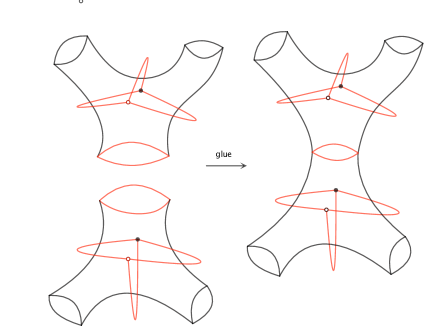
We would like to make a simple remark about the correlation function of 2d Toda field theory using our result (using the 2d/4d correspondence, the line operator on the Riemann surface will also be the observables of 2d Toda field theory.). Since the fourth punctured sphere can be derived by gluing two three punctured spheres, and the gluing only uses the line operator around the puncture, see figure. 32, and internal web operator is not used in gluing. In the 2d CFT interpretation, this means that the correlation function can be built from three point function, and the gluing is simple, which is consistent with 2d OPE. The nontrivial part of Toda field theory (counterpart of higher rank field theory) is that the three point function is complicated, as is manifested by the non-trivial line operators. The nice thing about the gluing picture is that once we understand the quantization of three punctured sphere, we should be able to understand the quantization of Toda field theory defined on any Riemann surface.

Figure 32: The gluing of two three punctured spheres is achieved by using the line operator around the puncture.

4.3 Disc with marked points

Let’s consider a disc with marked points, which describes 4d Argyres-Douglas theory [28]. The special requirement is: one need to ensure that the tropical $a$ coordinates of boundary quiver nodes to be zero, as we only counter the internal quiver nodes in studying of 4d $\mathcal{N}=2$ theory. Another important rule is that for the curve connected with two boundary points, the canonical map is defined as

$$\text{I}(l)=\begin{pmatrix}1&0&0\\ \end{pmatrix}*M*\begin{pmatrix}1\\ 0\\ 0\end{pmatrix},$$ (77)

here $M$ is the monodromy around the path and we set the boundary coordinates to be one in the end, so the answer does not depend on the boundary coordinates.

For simplicity, let’s consider $A_{2}$ theory on a disc with four marked points, which actually represents $D_{4}$ Argyres-Douglas theory [28]. A lamination satisfying the above constraint is shown in figure. 33, and its tropical $a$ coordinates is also shown. The canonical map is very simple $\text{I}(T_{1})=X_{1}X_{3}$, which is actually the central element in the Poisson structure (consider only the quiver nodes insider the quadrilateral). Another lamination using web is shown in figure. 33, and the canonical map of $W$ and the other two curves are

$$\text{I}(W)=\frac{X_{1}^{1/3}X_{2}}{X_{3}^{1/3}}+X_{1}^{1/3}X_{2}X_{3}^{2/3}+X_{1}^{1/3}X_{2}X_{3}^{2/3}X_{4},$$

$$\text{I}(A)=X_{1}^{-2/3}X_{3}^{-1/3}X_{2}^{-1/3}X_{4}^{-1/3},~{}~{}~{}~{}~{}~{}\text{I}(B)=X_{1}^{-2/3}X_{3}^{-1/3}X_{2}^{-2/3}X_{4}^{-2/3},$$ (78)

so the canonical map of this lamination is

$$\text{I}(T_{2})=\text{I}(W)*\text{I}(A)*\text{I}(B)=\frac{1}{\text{X}_{1}}+\frac{1}{\text{X}_{1}\text{X}_{4}}+\frac{1}{\text{X}_{1}\text{X}_{3}\text{X}_{4}}.$$ (79)

Figure 33: Left: two laminations on fourth punctured disc of $A_{2}$ theory. Right: The tropical $a$ coordinates of these two laminations.

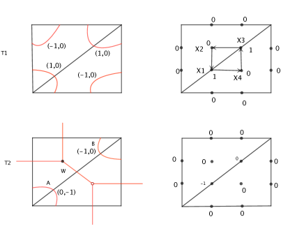
The same theory can be constructed using $A_{1}$ theory on a disc with four marked points and one bulk puncture, and the triangulation which give the same quiver as $A_{2}$ triangulations are shown in figure. 34. The lamination with the same tropical $a$ coordinates of $T_{2}$ is found using the reconstruction procedure described in section 2, see figure. 34. The canonical map of this lamination $T_{3}$ is found by using the monodromy representation of the $\text{SU}(2)$ local system described in section 2:

$$\text{I}(\text{A})=X_{1}^{-{1\over 2}},~{}~{}~{}\text{I}(\text{B})=X_{1}^{-{1\over 2}}X_{2}^{-{1\over 2}}X_{3}^{-{1\over 2}}X_{4}^{-{1\over 2}},~{}~{}\text{I}(\text{C})=X_{2}^{{1\over 2}}X_{3}^{{1\over 2}}X_{4}^{{1\over 2}}+X_{2}^{{1\over 2}}X_{3}^{{1\over 2}}X_{4}^{-{1\over 2}}+X_{2}^{{1\over 2}}X_{3}^{-{1\over 2}}X_{4}^{-{1\over 2}},$$ (80)

and the canonical map for this lamination is

$$\text{I}(T_{3})=\text{I}(\text{A})*\text{I}(\text{B})*\text{I}(\text{C})=\frac{1}{\text{X}_{1}}+\frac{1}{\text{X}_{1}\text{X}_{4}}+\frac{1}{\text{X}_{1}\text{X}_{3}\text{X}_{4}}.$$ (81)

Remarkably, this is equal to the answer found using $\text{SU}(3)$ representation. This result is clearly a very strong evidence that our generalization of lamination to higher rank theory is correct.

Figure 34: A $A_{1}$ lamination which gives the same tropical $a$ coordinates as the lamination $T_{2}$.

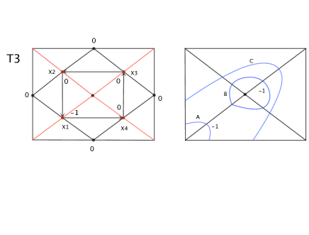
5 Conclusion

In this paper, we initiated a systematical study of half-BPS line operators of 4d $\mathcal{N}=2$ theory (theory of class ${\cal S}$) defined using full defects. Although the basic building blocks like line segments, three junctions are described for any $N$, we mainly focused on $A_{2}$ and $A_{3}$ theories, it would be interesting to further study general cases, i.e. giving the full Skein relations, finding the construction and reconstruction procedure as we did for $A_{2}$ case, etc. There are many other open questions and further generalizations:

• We found the canonical map of line operators using OPE, which is straightforward but tedious. It would be very useful if the answer can be directly found using web picture. This is important for $T_{N}$ theory as the OPE method is not applicable.

• It would be interesting to further study the OPE and general properties of the integer coefficients like its support and value. These results are useful in checking the conjectures given in [39]. It is also interesting to compare our results with the OPE of Wilson-’t Hooft operators studied in the context of $\mathcal{N}=4$ SYM [35, 40, 41, 42] and three dimensional theory [43].

• The non-full puncture case is worth to pursue, since in this case there are theories with Lagrangian descriptions and many field theory results are available [44, 45, 46, 47] (see also some results using Toda field theory [48, 49]). The basic tools like junctions, Skein relations should still be valid, and the cluster coordinates are given in [32, 28] which can be used to parameterize the line operators, etc; The main difficulty is that there are no monodromy calculation tools available, so we don’t know how to get the canonical map, currently we are trying to deal with this problem [50];

• Finally, it would be interesting to study various physical quantities related to the line operators, i.e. Superconformal index (see [51] for some $A_{1}$ cases), framed BPS states, $S^{4}$ partition function in the presence of line operators (see [52, 53] for $A_{1}$ theory with Lagrangian description) etc; it is also interesting to study how the line operator labels change under the pants decomposition, which would be a nice justification of $S$ duality.

One actually need a quantum version of line operators to answer many questions raised above. The quantum deformations of the line operator can be studied using quantum cluster algebra [39], for the $A_{1}$ case, see [27, 10, 54]. A complete treatment about these quantum line operators of higher rank case will be given in a future publication [55].

In this paper, we mainly focus on $A$ lamination and do not touch $X$ lamination. The main difference is the webs of $X$ lamination can end on bulk punctures. Such $X$ lamination is important in representing 4d BPS states in the $A_{1}$ case [56]. Naively, we expect the higher rank $X$ lamination should also give the 4d BPS states, and such interpretation matches perfectly with the expectation from the BPS quiver approach in some special cases we check, and we hope to come to this point in the near future.

The three junctions play a crucial role in our construction, and our derivation is based on the canonical map, cluster coordinates, etc. It would be interesting to see whether it can be realized as the one quarter BPS surface operator of $(2,0)$ theory. Similar web-like objects in M theory have been studied in [57, 58, 59], it is interesting to see if there is any relations between the junctions (superficially it seems that the number of junctions in our case is smaller than theirs.), see also the quarter BPS supergravity solutions related to M2 branes in [60]. If these webs can indeed be realized as quarter BPS surface operators, we expect them to be important in understanding the dynamics of $(2,0)$ theory.

Figure 35: The use of line (web) operators.

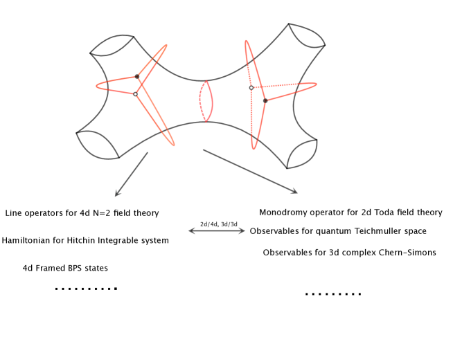
These line operators would have a lot of applications in various physical contexts due to the magical six dimensional construction, see figure. 35. It seems that all of them can be pursued using our result, and it would be exciting to do some concrete calculations.

Our work also has a lot of direct relations to mathematics. Firstly our web structure seems to be the geometric picture for the higher lamination proposed in [27, 39] (see also recent work on geometric realization of higher lamination using affine Grassmannia [61]); The web diagrams studied by us are also called tensor diagrams which are used to study cluster algebra in [62]. Secondly it is amusing to note that our Skein relations coincide with the one used in the study of Khovanov homology, see [63, 64], it would be interesting to see if there is any deep connection. Thirdly the OPE of Wilson and t’Hooft loops [35] and quantization of Hitchin integrable system [65] play an important role in the study of Geometric Langlands duality, Our results are both related to the OPE of line operators and quantization of Hitchin integrable system, and it is interesting to see if there are any potential applications.

Acknowledgments

We thank Tudor Dimorfte, Davide Gaiotto, Juan Maldacena, Edward Witten, Yuji Tachikawa, Masahito Yamazaki, Piljin Yi and Peng Zhao for help discussions. This research is supported in part by Zurich Financial services membership and by the U.S. Department of Energy, grant DE- FG02-90ER40542 (DX).

Appendix A Calculating monodromy

The cluster coordinates for higher rank theory defined using full punctures are found in [27]. It was conjectured that they are the BPS quiver for corresponding $\mathcal{N}=2$ theory in [32] which also gave a brane construction. One start with an ideal triangulation of bordered Riemann surface, and then further triangulate triangles in the triangulation. There are ${(N-1)(N-2)\over 2}$ new quiver nodes inside the triangle with three vertices $ABC$, and each internal quiver node can be labeled by three positive integers satisfying the condition

$$a+b+c=N,$$ (82)

here $a$ is defined as the distance to the dual side of the vertices $A$, etc, see figure. 36.

Figure 36: Top: the monodromy graph. Bottom: the label for coordinates inside a triangle, here the first index means the distance to the dual edge of vertex $A$.

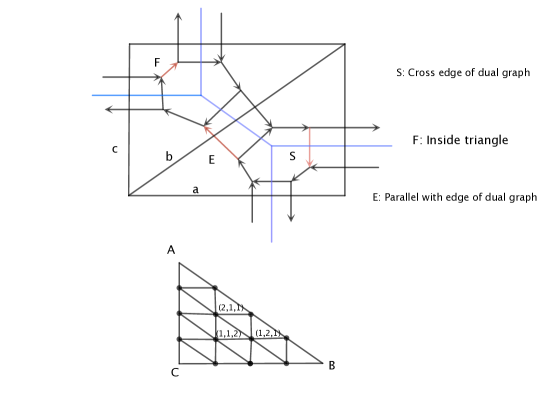
Let’s now summarize the ingredients for calculating the monodromy of higher rank local system following Fock and Goncharov [27]. For each triangulation, one can construct a dual graph: put one trivalent vertex inside each triangle and connect those trivalent vertices together to form a dual graph. We form a hexagon around each vertex and a square around each edge in the dual graph. We call dual graph together with the hexagons and squares as the monodromy graph. There are three types of edges in monodromy graph: S edge which intersects with the dual graph, E edge which is parallel with the edge of dual graph, and F edge which is inside the triangle, see figure. 36. We choose an orientation for edges in monodromy graph: the orientation is taken to be anti-clockwise for edges circling around the punctures, and all the edges in hexagon is taken to be in clockwise orientation.

The monodromy is calculated by assigning a $N\times N$ matrix to each edge in monodromy graph. The E type is a diagonal matrix depending on the coordinates on the edge of the triangulation with which edge E intersects:

$$E(\mathbb{a})[N]=\text{diag}(a_{0}a_{1}a_{2}...a_{N-1},a_{1}a_{2}...a_{N-1},\ldots,a_{N-1},1),$$ (83)

where the starting point for the label is taken as the vertex where edge $E$ circles around, see figure. 37. Notice that the matrix for other edge parallel with $E$ is denoted as $E(\bar{a})$ since we have different labeling for the coordinates. The coordinates $\bar{\mathbb{a}}$ are related to the $a$ coordinates as

$$\bar{\mathbb{a}}_{0}=a_{N-1},\ldots,\bar{\mathbb{a}}_{j}=a_{N-j-1},\ldots,\bar{\mathbb{a}}_{N-1}=a_{0}.$$ (84)

The $S$ Matrix also has a simple form:

$$S_{i,j}[N]=\begin{cases}(-1)^{i-1}~{}~{}j=N+1-i\\ 0\end{cases}$$ (85)

The F(ace) matrix is more complicated and it is composed by $F_{i}$ and $H_{i}$ matrix. The $H_{i}$ matrix is a diagonal one which has the form depending on position of the internal quiver node:

$$H_{i}(x)=\text{diag}(\underbrace{x,x,x}_{i},1,\ldots,1),$$ (86)

and $F_{i}$ matrix is defined as

$$(F_{i})_{m,n}=\begin{cases}1~{}\text{if}~{}m=n,~{}\text{or}~{}m=i~{}n=i-1\\ 0\end{cases}$$ (87)

So $F_{i}$ matrix is a lower triangular matrix with entry $one$ on the diagonal. Using the above two building blocks, the F(ace) matrix is expressed as

$$F[x,N]=\prod_{j=N-1}^{1}(\prod_{i=j-1}^{N-2}(H_{i+1}(X_{N-i-2,i-j,j-1})F_{i})F_{N-1}).$$ (88)

Notice that here an internal quiver node is labeled by three integers satisfying $a+b+c=N-3$, which is given by subtracting one from our previous labeling. For small $N$, the matrices are

$$F[x,2]=F_{1},~{}~{}~{}F[x,3]=F_{2}H_{2}(X_{0,0,0})F_{1}F_{2},$$

$$F[x,4]=F_{3}H_{3}(X_{0,1,0})F_{2}F_{3}H_{2}(X_{1,0,0})F_{1}H_{3}(X_{0,0,1})F_{2}F_{3}.$$ (89)

There is an easy way of remembering this sequence by looking at the quiver diagram in figure. 36. If the monodromy path is going from edge $AB$ to $AC$, then the above product is decomposed into $N-1$ steps. In each step, each quiver node on the line parallel to edge $AC$ contribute a factor $H_{i+1}F_{i}$, where $i$ is the distance to vertex $A$ of that quiver node. In each step, the sequence of product is to start from top to bottom, see figure. 37 for the arrows indicating the order of product; finally one need to add a matrix $F_{N-1}$ at the end in each step.

Figure 37: Top: the labeling for the coordinates on the edge with which $E$ intersects, and this labeling is used in the calculation of the monodromy. Bottom: the rule of remembering the formula for calculating the F matrix going from $AB$ to $AC$.

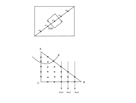
One should be really careful about the fact that the labeling of quiver nodes are quite different if the path is going through the other vertex of the triangle, so it is better to use different letters for the face matrix inside the same triangle, say $X,\bar{X},\bar{\bar{X}}$, and finally one should relate three set of coordinates by looking at their positions, say $X_{a,b,c}=\bar{X}_{b,a,c}$, etc.

The above matrices are the basic ingredients for calculating the monodromy, and if a path goes in opposite direction as the chosen orientation, we just use the inverse of above matrices. The monodromy around the square and the hexagon is an identity matrix up to a constant scalar, therefore the monodromy only depends on the homotopy class up to a complex scalar, and it defines a $\text{PGL}(N,C)$ local system. The monodromy for the $\text{SL}(N,C)$ local system is defined as

$$I(l)=|\text{Det}(M)^{-1/N}\text{Tr}(M)|.$$ (90)

here we take the absolute value to make sure that all the expressions are positive.

Appendix B Collection of canonical maps

For $A_{2}$ theory defined on once punctured torus, there are eight nontrivial generators. The quivers and the geometric representations for these eight line operators are shown in figure. 11 and 15. From the quiver, one can read the Poisson brackets for cluster coordinates, and one then use them to calculate the Poisson structure between the line operators combining the explicit expression of canonical map. We collect canonical maps for these eight generators, and the interested reader can do all kinds of calculations presented in the paper.

$$\mbox{I}(\mbox{L}_{1})={1\over{x^{2/3}y^{1/3}a_{0}^{1/3}a_{1}^{2/3}b_{0}^{1/3}b_{1}^{2/3}}}+{{b_{1}^{1/3}}\over{x^{2/3}y^{1/3}a_{0}^{1/3}a_{1}^{2/3}b_{0}^{1/3}}}+\frac{x^{1/3}b_{1}^{1/3}}{y^{1/3}a_{0}^{1/3}a_{1}^{2/3}b_{0}^{1/3}}+\frac{x^{1/3}a_{1}^{1/3}b_{1}^{1/3}}{y^{1/3}a_{0}^{1/3}b_{0}^{1/3}}+$$

$$\frac{x^{1/3}b_{0}^{2/3}b_{1}^{1/3}}{y^{1/3}a_{0}^{1/3}a_{1}^{2/3}}+\frac{x^{1/3}a_{1}^{1/3}b_{0}^{2/3}b_{1}^{1/3}}{y^{1/3}a_{0}^{1/3}}+\frac{x^{1/3}y^{2/3}a_{1}^{1/3}b_{0}^{2/3}b_{1}^{1/3}}{a_{0}^{1/3}}+x^{1/3}y^{2/3}a_{0}^{2/3}a_{1}^{1/3}b_{0}^{2/3}b_{1}^{1/3}$$ (91)

$$\mbox{I}(\mbox{L}_{2})=\frac{1}{x^{1/3}y^{2/3}a_{0}^{2/3}a_{1}^{1/3}b_{0}^{2/3}b_{1}^{1/3}}+\frac{b_{0}^{1/3}}{x^{1/3}y^{2/3}a_{0}^{2/3}a_{1}^{1/3}b_{1}^{1/3}}+\frac{y^{1/3}b_{0}^{1/3}}{x^{1/3}a_{0}^{2/3}a_{1}^{1/3}b_{1}^{1/3}}+\frac{y^{1/3}a_{0}^{1/3}b_{0}^{1/3}}{x^{1/3}a_{1}^{1/3}b_{1}^{1/3}}+$$

$$\frac{y^{1/3}b_{0}^{1/3}b_{1}^{2/3}}{x^{1/3}a_{0}^{2/3}a_{1}^{1/3}}+\frac{y^{1/3}a_{0}^{1/3}b_{0}^{1/3}b_{1}^{2/3}}{x^{1/3}a_{1}^{1/3}}+\frac{x^{2/3}y^{1/3}a_{0}^{1/3}b_{0}^{1/3}b_{1}^{2/3}}{a_{1}^{1/3}}+x^{2/3}y^{1/3}a_{0}^{1/3}a_{1}^{2/3}b_{0}^{1/3}b_{1}^{2/3}$$ (92)

$$\mbox{I}(\mbox{M}_{1})=\frac{1}{x^{1/3}y^{2/3}b_{0}^{1/3}b_{1}^{2/3}c_{0}^{1/3}c_{1}^{2/3}}+\frac{c_{1}^{1/3}}{x^{1/3}y^{2/3}b_{0}^{1/3}b_{1}^{2/3}c_{0}^{1/3}}+\frac{y^{1/3}c_{1}^{1/3}}{x^{1/3}b_{0}^{1/3}b_{1}^{2/3}c_{0}^{1/3}}+\frac{y^{1/3}b_{1}^{1/3}c_{1}^{1/3}}{x^{1/3}b_{0}^{1/3}c_{0}^{1/3}}$$

$$+\frac{y^{1/3}c_{0}^{2/3}c_{1}^{1/3}}{x^{1/3}b_{0}^{1/3}b_{1}^{2/3}}+\frac{y^{1/3}b_{1}^{1/3}c_{0}^{2/3}c_{1}^{1/3}}{x^{1/3}b_{0}^{1/3}}+\frac{x^{2/3}y^{1/3}b_{1}^{1/3}c_{0}^{2/3}c_{1}^{1/3}}{b_{0}^{1/3}}+x^{2/3}y^{1/3}b_{0}^{2/3}b_{1}^{1/3}c_{0}^{2/3}c_{1}^{1/3}$$ (93)

$$\mbox{I}(\mbox{M}_{2})=\frac{1}{x^{2/3}y^{1/3}b_{0}^{2/3}b_{1}^{1/3}c_{0}^{2/3}c_{1}^{1/3}}+\frac{c_{0}^{1/3}}{x^{2/3}y^{1/3}b_{0}^{2/3}b_{1}^{1/3}c_{1}^{1/3}}+\frac{x^{1/3}c_{0}^{1/3}}{y^{1/3}b_{0}^{2/3}b_{1}^{1/3}c_{1}^{1/3}}+\frac{x^{1/3}b_{0}^{1/3}c_{0}^{1/3}}{y^{1/3}b_{1}^{1/3}c_{1}^{1/3}}$$

$$+\frac{x^{1/3}c_{0}^{1/3}c_{1}^{2/3}}{y^{1/3}b_{0}^{2/3}b_{1}^{1/3}}+\frac{x^{1/3}b_{0}^{1/3}c_{0}^{1/3}c_{1}^{2/3}}{y^{1/3}b_{1}^{1/3}}+\frac{x^{1/3}y^{2/3}b_{0}^{1/3}c_{0}^{1/3}c_{1}^{2/3}}{b_{1}^{1/3}}+x^{1/3}y^{2/3}b_{0}^{1/3}b_{1}^{2/3}c_{0}^{1/3}c_{1}^{2/3}$$ (94)

$$\mbox{I}(\mbox{C}_{1})=\frac{1}{x^{1/3}y^{2/3}a_{0}^{1/3}a_{1}^{2/3}c_{0}^{2/3}c_{1}^{1/3}}+\frac{a_{1}^{1/3}}{x^{1/3}y^{2/3}a_{0}^{1/3}c_{0}^{2/3}c_{1}^{1/3}}+\frac{y^{1/3}a_{1}^{1/3}}{x^{1/3}a_{0}^{1/3}c_{0}^{2/3}c_{1}^{1/3}}+\frac{y^{1/3}a_{0}^{2/3}a_{1}^{1/3}}{x^{1/3}c_{0}^{2/3}c_{1}^{1/3}}$$

$$+\frac{y^{1/3}a_{1}^{1/3}c_{0}^{1/3}}{x^{1/3}a_{0}^{1/3}c_{1}^{1/3}}+\frac{y^{1/3}a_{0}^{2/3}a_{1}^{1/3}c_{0}^{1/3}}{x^{1/3}c_{1}^{1/3}}+\frac{x^{2/3}y^{1/3}a_{0}^{2/3}a_{1}^{1/3}c_{0}^{1/3}}{c_{1}^{1/3}}+x^{2/3}y^{1/3}a_{0}^{2/3}a_{1}^{1/3}c_{0}^{1/3}c_{1}^{2/3}$$ (95)

$$\mbox{I}(\mbox{C}_{2})=\frac{1}{x^{2/3}y^{1/3}a_{0}^{2/3}a_{1}^{1/3}c_{0}^{1/3}c_{1}^{2/3}}+\frac{a_{0}^{1/3}}{x^{2/3}y^{1/3}a_{1}^{1/3}c_{0}^{1/3}c_{1}^{2/3}}+\frac{x^{1/3}a_{0}^{1/3}}{y^{1/3}a_{1}^{1/3}c_{0}^{1/3}c_{1}^{2/3}}+\frac{x^{1/3}a_{0}^{1/3}a_{1}^{2/3}}{y^{1/3}c_{0}^{1/3}c_{1}^{2/3}}$$

$$+\frac{x^{1/3}a_{0}^{1/3}c_{1}^{1/3}}{y^{1/3}a_{1}^{1/3}c_{0}^{1/3}}+\frac{x^{1/3}a_{0}^{1/3}a_{1}^{2/3}c_{1}^{1/3}}{y^{1/3}c_{0}^{1/3}}+\frac{x^{1/3}y^{2/3}a_{0}^{1/3}a_{1}^{2/3}c_{1}^{1/3}}{c_{0}^{1/3}}+x^{1/3}y^{2/3}a_{0}^{1/3}a_{1}^{2/3}c_{0}^{2/3}c_{1}^{1/3}$$ (96)

$$\mbox{I}(I_{1})=\frac{a_{1}^{1/3}b_{0}^{1/3}}{a_{0}^{1/3}b_{1}^{1/3}c_{0}^{1/3}c_{1}^{2/3}}+\frac{a_{0}^{2/3}a_{1}^{1/3}b_{0}^{1/3}}{b_{1}^{1/3}c_{0}^{1/3}c_{1}^{2/3}}+\frac{a_{1}^{1/3}c_{1}^{1/3}}{a_{0}^{1/3}b_{0}^{2/3}b_{1}^{1/3}c_{0}^{1/3}}+\frac{b_{0}^{1/3}c_{1}^{1/3}}{a_{0}^{1/3}a_{1}^{2/3}b_{1}^{1/3}c_{0}^{1/3}}$$

$$+\frac{2a_{1}^{1/3}b_{0}^{1/3}c_{1}^{1/3}}{a_{0}^{1/3}b_{1}^{1/3}c_{0}^{1/3}}+\frac{a_{0}^{2/3}a_{1}^{1/3}b_{0}^{1/3}c_{1}^{1/3}}{b_{1}^{1/3}c_{0}^{1/3}}+\frac{b_{0}^{1/3}b_{1}^{2/3}c_{1}^{1/3}}{a_{0}^{1/3}a_{1}^{2/3}c_{0}^{1/3}}+\frac{a_{1}^{1/3}b_{0}^{1/3}b_{1}^{2/3}c_{1}^{1/3}}{a_{0}^{1/3}c_{0}^{1/3}}$$

$$+\frac{a_{1}^{1/3}c_{0}^{2/3}c_{1}^{1/3}}{a_{0}^{1/3}b_{0}^{2/3}b_{1}^{1/3}}+\frac{a_{1}^{1/3}b_{0}^{1/3}c_{0}^{2/3}c_{1}^{1/3}}{a_{0}^{1/3}b_{1}^{1/3}}+\frac{1}{a_{0}^{1/3}a_{1}^{2/3}b_{0}^{2/3}b_{1}^{1/3}c_{0}^{1/3}c_{1}^{2/3}y}+\frac{a_{1}^{1/3}}{a_{0}^{1/3}b_{0}^{2/3}b_{1}^{1/3}c_{0}^{1/3}c_{1}^{2/3}y}$$

$$+\frac{b_{0}^{1/3}}{a_{0}^{1/3}a_{1}^{2/3}b_{1}^{1/3}c_{0}^{1/3}c_{1}^{2/3}y}+\frac{a_{1}^{1/3}b_{0}^{1/3}}{a_{0}^{1/3}b_{1}^{1/3}c_{0}^{1/3}c_{1}^{2/3}y}+\frac{c_{1}^{1/3}}{a_{0}^{1/3}a_{1}^{2/3}b_{0}^{2/3}b_{1}^{1/3}c_{0}^{1/3}y}+\frac{a_{1}^{1/3}c_{1}^{1/3}}{a_{0}^{1/3}b_{0}^{2/3}b_{1}^{1/3}c_{0}^{1/3}y}$$

$$+\frac{b_{0}^{1/3}c_{1}^{1/3}}{a_{0}^{1/3}a_{1}^{2/3}b_{1}^{1/3}c_{0}^{1/3}y}+\frac{a_{1}^{1/3}b_{0}^{1/3}c_{1}^{1/3}}{a_{0}^{1/3}b_{1}^{1/3}c_{0}^{1/3}y}+\frac{1}{a_{0}^{1/3}a_{1}^{2/3}b_{0}^{2/3}b_{1}^{1/3}c_{0}^{1/3}c_{1}^{2/3}xy}+\frac{a_{1}^{1/3}b_{0}^{1/3}c_{1}^{1/3}y}{a_{0}^{1/3}b_{1}^{1/3}c_{0}^{1/3}}$$

$$+\frac{a_{0}^{2/3}a_{1}^{1/3}b_{0}^{1/3}c_{1}^{1/3}y}{b_{1}^{1/3}c_{0}^{1/3}}+\frac{a_{1}^{1/3}b_{0}^{1/3}b_{1}^{2/3}c_{1}^{1/3}y}{a_{0}^{1/3}c_{0}^{1/3}}+\frac{a_{0}^{2/3}a_{1}^{1/3}b_{0}^{1/3}b_{1}^{2/3}c_{1}^{1/3}y}{c_{0}^{1/3}}+\frac{a_{1}^{1/3}b_{0}^{1/3}c_{0}^{2/3}c_{1}^{1/3}y}{a_{0}^{1/3}b_{1}^{1/3}}$$

$$+\frac{a_{0}^{2/3}a_{1}^{1/3}b_{0}^{1/3}c_{0}^{2/3}c_{1}^{1/3}y}{b_{1}^{1/3}}+\frac{a_{1}^{1/3}b_{0}^{1/3}b_{1}^{2/3}c_{0}^{2/3}c_{1}^{1/3}y}{a_{0}^{1/3}}+a_{0}^{2/3}a_{1}^{1/3}b_{0}^{1/3}b_{1}^{2/3}c_{0}^{2/3}c_{1}^{1/3}y+a_{0}^{2/3}a_{1}^{1/3}b_{0}^{1/3}b_{1}^{2/3}c_{0}^{2/3}c_{1}^{1/3}xy$$ (97)

$$\mbox{I}(I_{2})=$$

$$\frac{1}{xa_{0}^{2/3}a_{1}^{1/3}b_{0}^{1/3}b_{1}^{2/3}c_{0}^{2/3}c_{1}^{1/3}}+\frac{1}{xya_{0}^{2/3}a_{1}^{1/3}b_{0}^{1/3}b_{1}^{2/3}c_{0}^{2/3}c_{1}^{1/3}}+\frac{a_{0}^{1/3}}{xa_{1}^{1/3}b_{0}^{1/3}b_{1}^{2/3}c_{0}^{2/3}c_{1}^{1/3}}+\frac{b_{1}^{1/3}}{xa_{0}^{2/3}a_{1}^{1/3}b_{0}^{1/3}c_{0}^{2/3}c_{1}^{1/3}}$$

$$+\frac{a_{0}^{1/3}b_{1}^{1/3}}{a_{1}^{1/3}b_{0}^{1/3}c_{0}^{2/3}c_{1}^{1/3}}+\frac{a_{0}^{1/3}b_{1}^{1/3}}{xa_{1}^{1/3}b_{0}^{1/3}c_{0}^{2/3}c_{1}^{1/3}}+\frac{a_{0}^{1/3}a_{1}^{2/3}b_{1}^{1/3}}{b_{0}^{1/3}c_{0}^{2/3}c_{1}^{1/3}}+\frac{c_{0}^{1/3}}{xa_{0}^{2/3}a_{1}^{1/3}b_{0}^{1/3}b_{1}^{2/3}c_{1}^{1/3}}$$

$$+\frac{a_{0}^{1/3}c_{0}^{1/3}}{a_{1}^{1/3}b_{0}^{1/3}b_{1}^{2/3}c_{1}^{1/3}}+\frac{a_{0}^{1/3}c_{0}^{1/3}}{xa_{1}^{1/3}b_{0}^{1/3}b_{1}^{2/3}c_{1}^{1/3}}+\frac{b_{1}^{1/3}c_{0}^{1/3}}{a_{0}^{2/3}a_{1}^{1/3}b_{0}^{1/3}c_{1}^{1/3}}+\frac{b_{1}^{1/3}c_{0}^{1/3}}{xa_{0}^{2/3}a_{1}^{1/3}b_{0}^{1/3}c_{1}^{1/3}}$$

$$+\frac{2a_{0}^{1/3}b_{1}^{1/3}c_{0}^{1/3}}{a_{1}^{1/3}b_{0}^{1/3}c_{1}^{1/3}}+\frac{a_{0}^{1/3}b_{1}^{1/3}c_{0}^{1/3}}{xa_{1}^{1/3}b_{0}^{1/3}c_{1}^{1/3}}+\frac{xa_{0}^{1/3}b_{1}^{1/3}c_{0}^{1/3}}{a_{1}^{1/3}b_{0}^{1/3}c_{1}^{1/3}}+\frac{a_{0}^{1/3}a_{1}^{2/3}b_{1}^{1/3}c_{0}^{1/3}}{b_{0}^{1/3}c_{1}^{1/3}}$$

$$+\frac{xa_{0}^{1/3}a_{1}^{2/3}b_{1}^{1/3}c_{0}^{1/3}}{b_{0}^{1/3}c_{1}^{1/3}}+\frac{b_{0}^{2/3}b_{1}^{1/3}c_{0}^{1/3}}{a_{0}^{2/3}a_{1}^{1/3}c_{1}^{1/3}}+\frac{a_{0}^{1/3}b_{0}^{2/3}b_{1}^{1/3}c_{0}^{1/3}}{a_{1}^{1/3}c_{1}^{1/3}}+\frac{xa_{0}^{1/3}b_{0}^{2/3}b_{1}^{1/3}c_{0}^{1/3}}{a_{1}^{1/3}c_{1}^{1/3}}$$

$$+\frac{xa_{0}^{1/3}a_{1}^{2/3}b_{0}^{2/3}b_{1}^{1/3}c_{0}^{1/3}}{c_{1}^{1/3}}+\frac{a_{0}^{1/3}c_{0}^{1/3}c_{1}^{2/3}}{a_{1}^{1/3}b_{0}^{1/3}b_{1}^{2/3}}+\frac{a_{0}^{1/3}b_{1}^{1/3}c_{0}^{1/3}c_{1}^{2/3}}{a_{1}^{1/3}b_{0}^{1/3}}+\frac{xa_{0}^{1/3}b_{1}^{1/3}c_{0}^{1/3}c_{1}^{2/3}}{a_{1}^{1/3}b_{0}^{1/3}}$$

$$+\frac{xa_{0}^{1/3}a_{1}^{2/3}b_{1}^{1/3}c_{0}^{1/3}c_{1}^{2/3}}{b_{0}^{1/3}}+\frac{xa_{0}^{1/3}b_{0}^{2/3}b_{1}^{1/3}c_{0}^{1/3}c_{1}^{2/3}}{a_{1}^{1/3}}+xa_{0}^{1/3}a_{1}^{2/3}b_{0}^{2/3}b_{1}^{1/3}c_{0}^{1/3}c_{1}^{2/3}+xya_{0}^{1/3}a_{1}^{2/3}b_{0}^{2/3}b_{1}^{1/3}c_{0}^{1/3}c_{1}^{2/3}$$ (98)

$$\mbox{I}(2\omega_{1})$$

$$=\frac{1}{x^{4/3}y^{2/3}a_{0}^{2/3}a_{1}^{4/3}b_{0}^{2/3}b_{1}^{4/3}}+\frac{2}{x^{4/3}y^{2/3}a_{0}^{2/3}a_{1}^{4/3}b_{0}^{2/3}b_{1}^{1/3}}+\frac{2}{x^{1/3}y^{2/3}a_{0}^{2/3}a_{1}^{4/3}b_{0}^{2/3}b_{1}^{1/3}}+\frac{2b_{0}^{1/3}}{x^{1/3}y^{2/3}a_{0}^{2/3}a_{1}^{4/3}b_{1}^{1/3}}$$

$$+\frac{b_{1}^{2/3}}{x^{4/3}y^{2/3}a_{0}^{2/3}a_{1}^{4/3}b_{0}^{2/3}}+\frac{2b_{1}^{2/3}}{x^{1/3}y^{2/3}a_{0}^{2/3}a_{1}^{4/3}b_{0}^{2/3}}+\frac{x^{2/3}b_{1}^{2/3}}{y^{2/3}a_{0}^{2/3}a_{1}^{4/3}b_{0}^{2/3}}+\frac{2b_{1}^{2/3}}{x^{1/3}y^{2/3}a_{0}^{2/3}a_{1}^{1/3}b_{0}^{2/3}}$$

$$+\frac{2x^{2/3}b_{1}^{2/3}}{y^{2/3}a_{0}^{2/3}a_{1}^{1/3}b_{0}^{2/3}}+\frac{x^{2/3}a_{1}^{2/3}b_{1}^{2/3}}{y^{2/3}a_{0}^{2/3}b_{0}^{2/3}}+\frac{2b_{0}^{1/3}b_{1}^{2/3}}{x^{1/3}y^{2/3}a_{0}^{2/3}a_{1}^{4/3}}+\frac{2x^{2/3}b_{0}^{1/3}b_{1}^{2/3}}{y^{2/3}a_{0}^{2/3}a_{1}^{4/3}}+\frac{2b_{0}^{1/3}b_{1}^{2/3}}{x^{1/3}y^{2/3}a_{0}^{2/3}a_{1}^{1/3}}$$

$$+\frac{4x^{2/3}b_{0}^{1/3}b_{1}^{2/3}}{y^{2/3}a_{0}^{2/3}a_{1}^{1/3}}+\frac{2x^{2/3}y^{1/3}b_{0}^{1/3}b_{1}^{2/3}}{a_{0}^{2/3}a_{1}^{1/3}}\frac{2x^{2/3}a_{1}^{2/3}b_{0}^{1/3}b_{1}^{2/3}}{y^{2/3}a_{0}^{2/3}}+\frac{2x^{2/3}y^{1/3}a_{1}^{2/3}b_{0}^{1/3}b_{1}^{2/3}}{a_{0}^{2/3}}+$$

$$\frac{x^{2/3}b_{0}^{4/3}b_{1}^{2/3}}{y^{2/3}a_{0}^{2/3}a_{1}^{4/3}}+\frac{2x^{2/3}b_{0}^{4/3}b_{1}^{2/3}}{y^{2/3}a_{0}^{2/3}a_{1}^{1/3}}+\frac{2x^{2/3}y^{1/3}b_{0}^{4/3}b_{1}^{2/3}}{a_{0}^{2/3}a_{1}^{1/3}}+\frac{2x^{2/3}y^{1/3}a_{0}^{1/3}b_{0}^{4/3}b_{1}^{2/3}}{a_{1}^{1/3}}$$

$$+\frac{x^{2/3}a_{1}^{2/3}b_{0}^{4/3}b_{1}^{2/3}}{y^{2/3}a_{0}^{2/3}}+\frac{2x^{2/3}y^{1/3}a_{1}^{2/3}b_{0}^{4/3}b_{1}^{2/3}}{a_{0}^{2/3}}+\frac{x^{2/3}y^{4/3}a_{1}^{2/3}b_{0}^{4/3}b_{1}^{2/3}}{a_{0}^{2/3}}$$

$$+2x^{2/3}y^{1/3}a_{0}^{1/3}a_{1}^{2/3}b_{0}^{4/3}b_{1}^{2/3}+2x^{2/3}y^{4/3}a_{0}^{1/3}a_{1}^{2/3}b_{0}^{4/3}b_{1}^{2/3}+x^{2/3}y^{4/3}a_{0}^{4/3}a_{1}^{2/3}b_{0}^{4/3}b_{1}^{2/3}$$ (99)

References

- [1] A. M. Polyakov, “String theory and quark confinement,” Nucl.Phys.Proc.Suppl. 68 (1998) 1–8, arXiv:hep-th/9711002 [hep-th].
- [2] J. M. Maldacena, “Wilson loops in large N field theories,” Phys.Rev.Lett. 80 (1998) 4859–4862, arXiv:hep-th/9803002 [hep-th].
- [3] S.-J. Rey and J.-T. Yee, “Macroscopic strings as heavy quarks in large N gauge theory and anti-de Sitter supergravity,” Eur.Phys.J. C22 (2001) 379–394, arXiv:hep-th/9803001 [hep-th].
- [4] L. F. Alday and J. M. Maldacena, “Gluon scattering amplitudes at strong coupling,” JHEP 0706 (2007) 064, arXiv:0705.0303 [hep-th].
- [5] S. Caron-Huot, “Notes on the scattering amplitude / Wilson loop duality,” JHEP 1107 (2011) 058, arXiv:1010.1167 [hep-th].
- [6] D. Gaiotto, “ dualities,” arXiv:0904.2715 [hep-th].
- [7] D. Gaiotto, G. W. Moore, and A. Neitzke, “Wall-crossing, hitchin Systems, and the WKB approximation,” arXiv:0907.3987 [hep-th].
- [8] D. Xie, “General Argyres-Douglas Theory,” arXiv:1204.2270 [hep-th].
- [9] N. Drukker, D. R. Morrison, and T. Okuda, “Loop operators and S-duality from curves on Riemann surfaces,” JHEP 09 (2009) 031, arXiv:0907.2593 [hep-th].
- [10] D. Gaiotto, G. W. Moore, and A. Neitzke, “Framed BPS states,” arXiv:1006.0146 [hep-th].
- [11] N. A. Nekrasov and S. L. Shatashvili, “Quantization of integrable systems and four dimensional gauge theories,” arXiv:0908.4052 [hep-th].
- [12] N. Nekrasov, A. Rosly, and S. Shatashvili, “Darboux coordinates, Yang-Yang functional, and gauge theory,” Nucl. Phys. Proc. Suppl. 216 (2011) 69–93, arXiv:1103.3919 [hep-th].
- [13] N. Nekrasov and E. Witten, “The Omega deformation, branes, integrability, and liouville Theory,” JHEP 09 (2010) 092, arXiv:1002.0888 [hep-th].
- [14] Y. Ito, T. Okuda, and M. Taki, “Line operators on and quantization of the Hitchin moduli space,” JHEP 1204 (2012) 010, arXiv:1111.4221 [hep-th].
- [15] J. Teschner, “Quantization of the Hitchin moduli spaces, Liouville theory, and the geometric Langlands correspondence I,” Adv.Theor.Math.Phys. 15 (2011) 471–564, arXiv:1005.2846 [hep-th].
- [16] G. Vartanov and J. Teschner, “Supersymmetric gauge theories, quantization of moduli spaces of flat connections, and conformal field theory,” arXiv:1302.3778 [hep-th].
- [17] A. Strominger, “Open p-branes,” Phys.Lett. B383 (1996) 44–47, arXiv:hep-th/9512059 [hep-th].
- [18] D. E. Berenstein, R. Corrado, W. Fischler, and J. M. Maldacena, “The Operator product expansion for Wilson loops and surfaces in the large N limit,” Phys.Rev. D59 (1999) 105023, arXiv:hep-th/9809188 [hep-th].
- [19] C. R. Graham and E. Witten, “Conformal anomaly of submanifold observables in AdS / CFT correspondence,” Nucl.Phys. B546 (1999) 52–64, arXiv:hep-th/9901021 [hep-th].
- [20] V. V. Fock and A. B. Goncharov, “Dual teichmuller and lamination spaces,” arXiv preprint math/0510312 (2005) .
- [21] O. Lunin, “1/2-BPS states in M theory and defects in the dual CFTs,” JHEP 0710 (2007) 014, arXiv:0704.3442 [hep-th].
- [22] B. Chen, W. He, J.-B. Wu, and L. Zhang, “M5-branes and Wilson Surfaces,” JHEP 0708 (2007) 067, arXiv:0707.3978 [hep-th].
- [23] E. D’Hoker, J. Estes, and M. Gutperle, “Exact half-BPS Type IIB interface solutions. II. Flux solutions and multi-Janus,” JHEP 0706 (2007) 022, arXiv:0705.0024 [hep-th].
- [24] A. Kapustin, “Wilson-’t Hooft operators in four-dimensional gauge theories and S-duality,” Phys.Rev. D74 (2006) 025005, arXiv:hep-th/0501015 [hep-th].
- [25] N. Drukker, D. Gaiotto, and J. Gomis, “The Virtue of Defects in 4D Gauge Theories and 2D CFTs,” JHEP 1106 (2011) 025, arXiv:1003.1112 [hep-th].
- [26] L. F. Alday, D. Gaiotto, and Y. Tachikawa, “Liouville correlation functions from four-dimensional gauge theories,” Lett. Math. Phys. 91 (2010) 167–197, arXiv:0906.3219 [hep-th].
- [27] V. V. Fock and A. B. Goncharov, “Moduli spaces of local systems and higher teichmuller theory,”. \urlarXiv.org:math/0311149.
- [28] D. Xie, “Network, cluster coordinates and N = 2 theory II: Irregular singularity,” arXiv:1207.6112 [hep-th].
- [29] S. Cecotti and C. Vafa, “Classification of complete N=2 supersymmetric theories in 4 dimensions,” arXiv:1103.5832 [hep-th].
- [30] S. Fomin, M. Shapiro, and D. Thurston, “Cluster algebras and triangulated surfaces. part i: Cluster complexes,” ACTA MATHEMATICA 201 (2008) 83. \urlarXiv.org:math/0608367.
- [31] E. Witten, “Solutions of four-dimensional field theories via M-theory,” Nucl. Phys. B500 (1997) 3–42, arXiv:hep-th/9703166.
- [32] D. Xie, “Network, Cluster coordinates and N=2 theory I,” arXiv:1203.4573 [hep-th].
- [33] B. Feng, Y.-H. He, K. D. Kennaway, and C. Vafa, “Dimer models from mirror symmetry and quivering amoebae,” Adv.Theor.Math.Phys. 12 (2008) 489–545, arXiv:hep-th/0511287 [hep-th].
- [34] S. Fomin and A. Zelevinsky, “Cluster algebras I: Foundations,” J. Amer. Math. Soc. 15 (2002) 497–529, arXiv:math/0104151.
- [35] A. Kapustin and E. Witten, “Electric-Magnetic Duality And The Geometric Langlands Program,” Commun.Num.Theor.Phys. 1 (2007) 1–236, arXiv:hep-th/0604151 [hep-th].
- [36] D. Xie and M. Yamazaki, “Network and Seiberg Duality,” arXiv:1207.0811 [hep-th].
- [37] S. Franco, “Bipartite Field Theories: from D-Brane Probes to Scattering Amplitudes,” arXiv:1207.0807 [hep-th].
- [38] N. Arkani-Hamed, J. L. Bourjaily, F. Cachazo, A. B. Goncharov, A. Postnikov, and J. Trnka, “Scattering amplitudes and the positive grassmannian,” arXiv preprint arXiv:1212.5605 (2012) .
- [39] V. V. Fock and A. B. Goncharov, “Cluster ensembles, quantization and the dilogarithm,” math/0311245.
- [40] A. Kapustin and N. Saulina, “The Algebra of Wilson-’t Hooft operators,” Nucl.Phys. B814 (2009) 327–365, arXiv:0710.2097 [hep-th].
- [41] N. Saulina, “A note on Wilson-’t Hooft operators,” Nucl.Phys. B857 (2012) 153–171, arXiv:1110.3354 [hep-th].
- [42] R. Moraru and N. Saulina, “OPE of Wilson-’t Hooft operators in N=4 and N=2 SYM with gauge group G=PSU(3),” arXiv:1206.6896 [hep-th].
- [43] A. Kapustin and B. Willett, “Wilson loops in supersymmetric Chern-Simons-matter theories and duality,” arXiv:1302.2164 [hep-th].
- [44] A. Kapustin, “Holomorphic reduction of N=2 gauge theories, Wilson-’t Hooft operators, and S-duality,” arXiv:hep-th/0612119 [hep-th].
- [45] V. Pestun, “Localization of gauge theory on a four-sphere and supersymmetric Wilson loops,” arXiv:0712.2824 [hep-th].
- [46] J. Gomis, T. Okuda, and V. Pestun, “Exact Results for ’t Hooft Loops in Gauge Theories on ,” JHEP 1205 (2012) 141, arXiv:1105.2568 [hep-th].
- [47] S.-J. Rey and T. Suyama, “Exact Results and Holography of Wilson Loops in N=2 Superconformal (Quiver) Gauge Theories,” JHEP 1101 (2011) 136, arXiv:1001.0016 [hep-th].
- [48] J. Gomis and B. Le Floch, “’t Hooft Operators in Gauge Theory from Toda CFT,” JHEP 1111 (2011) 114, arXiv:1008.4139 [hep-th].
- [49] F. Passerini, “Gauge Theory Wilson Loops and Conformal Toda Field Theory,” JHEP 1003 (2010) 125, arXiv:1003.1151 [hep-th].
- [50] D. Xie, “Higher laminations, webs, and line operators ii: non-full puncture.,” Work in progress .
- [51] D. Gang, E. Koh, and K. Lee, “Line Operator Index on ,” JHEP 1205 (2012) 007, arXiv:1201.5539 [hep-th].
- [52] N. Drukker, J. Gomis, T. Okuda, and J. Teschner, “Gauge theory loop operators and liouville theory,” JHEP 1002 (2010) 057, arXiv:0909.1105 [hep-th].
- [53] L. F. Alday, D. Gaiotto, S. Gukov, Y. Tachikawa, and H. Verlinde, “Loop and surface operators in N=2 gauge theory and Liouville modular geometry,” JHEP 1001 (2010) 113, arXiv:0909.0945 [hep-th].
- [54] T. Dimofte and S. Gukov, “Chern-Simons Theory and S-duality,” arXiv:1106.4550 [hep-th].
- [55] D. Xie, “Quantum line operators,” To appear .
- [56] D. Xie, “BPS spectrum, wall crossing and quantum dilogarithm identity,” arXiv:1211.7071 [hep-th].
- [57] K.-M. Lee and H.-U. Yee, “BPS String Webs in the 6-dim (2,0) Theories,” JHEP 0703 (2007) 057, arXiv:hep-th/0606150 [hep-th].
- [58] S. Bolognesi and K. Lee, “1/4 BPS String Junctions and Problem in 6-dim (2,0) Superconformal Theories,” Phys.Rev. D84 (2011) 126018, arXiv:1105.5073 [hep-th].
- [59] D. Gaiotto, G. W. Moore, and A. Neitzke, “Spectral networks,” arXiv:1204.4824 [hep-th].
- [60] O. Lunin, “Brane webs and 1/4-BPS geometries,” JHEP 0809 (2008) 028, arXiv:0802.0735 [hep-th].
- [61] I. Le, “Higher laminations and affine buildings,” arXiv preprint arXiv:1209.0812 (2012) .
- [62] S. Fomin and P. Pylyavskyy, “Tensor diagrams and cluster algebras,” arXiv preprint arXiv:1210.1888 (2012) .
- [63] G. Kuperberg, “Spiders for rank 2 lie algebras,” Communications in mathematical physics 180 (1996) no. 1, 109–151.
- [64] M. Khovanov, “sl (3) link homology,” Algebr. Geom. Topol 4 (2004) 1045–1081.
- [65] V. D. A. Beilinson, “Quantization of hitchin’s integrable system and hecke eigensheaves,” http://www.math.uchicago.edu/ mitya/langlands/hitchin/BD-hitchin.pdf. .