Controlling the position of traveling waves in reaction-diffusion systems

Abstract

We present a method to control the position as a function of time of one-dimensional traveling wave solutions to reaction-diffusion systems according to a pre-specified protocol of motion. Given this protocol, the control function is found as the solution of a perturbatively derived integral equation. Two cases are considered. First, we derive an analytical expression for the space ($x$) and time ($t$) dependent control function $f\left(x,t\right)$ that is valid for arbitrary protocols and many reaction-diffusion systems. These results are close to numerically computed optimal controls. Second, for stationary control of traveling waves in one-component systems, the integral equation reduces to a Fredholm integral equation of the first kind. In both cases, the control can be expressed in terms of the uncontrolled wave profile and its propagation velocity, rendering detailed knowledge of the reaction kinetics unnecessary.

A variety of approaches have been developed for the purposeful manipulation of reaction-diffusion (RD) systems as e.g. the application of feedback-mediated control loops with and without delays, external spatio-temporal forcing or imposing heterogeneities and geometric constraints on the medium mikhailov2006control ; *vanag2008design. For example, unstable patterns can be stabilized by global feedback control, as was shown in experiments with the light-sensitive Belousov-Zhabotinsky (BZ) reaction mihaliuk2002feedback ; *Zykov2004global; *zykov2004feedback. Two feedback loops were used to stabilize unstable wave segments and to guide their propagation direction sakurai2002design . Position control, or dragging, of a traveling chemical pulse wolff2003gentle on an addressable catalyst surface wolff2001spatiotemporal was accomplished experimentally by a moving, localized temperature heterogeneity. Dragging of fronts in chemical and phase transitions models as well as targeted transfer of nonlinear Schrödinger pulses by moving heterogeneities was studied in kevrekidis2004dragging ; *nistazakis2002targeted; *malomed2002pulled.
Many of these control methods rely on extensive knowledge about the system to be controlled. Feedback control necessitates continuous monitoring of the system, while optimal control troltzsch2010optimal ; *jorge1999numerical; *theissen2006optimale; *buchholz2013on requires full knowledge of the underlying partial differential equations (PDE) governing the system’s evolution in time and space.
In this Letter we propose a method which partially overcomes the aforementioned difficulties and still compares favorably with a competing control method, namely optimal control. We consider the problem to control the position over time of one-dimensional traveling waves (TW) by spatio-temporal forcing. The starting point is a system of RD equations

$$\partial_{t}\mathbf{u} =D\partial_{x}^{2}\mathbf{u}+\mathbf{R}\left(\mathbf{u}\right)+\epsilon\mathcal{G}\left(\mathbf{u}\right)\mathbf{f}\left(x,t\right),$$ (1)

where $D$ is a diagonal matrix of constant diffusion coefficients, $\mathbf{f}$ is a spatio-temporal perturbation, $\mathcal{G}$ a (possibly $\mathbf{u}$-dependent) coupling matrix, and $\mathbf{R}$ the nonlinear reaction kinetics. The unperturbed ($\epsilon=0$) solution $\mathbf{U}_{c}\left(\xi\right)$, $\xi=x-ct$, is assumed to be a TW, stationary in the reference frame co-moving with velocity $c$, so that

$$D\partial_{\xi}^{2}\mathbf{U}_{c}\left(\xi\right)+c\partial_{\xi}\mathbf{U}_{c}\left(\xi\right)+\mathbf{R}\left(\mathbf{U}_{c}\left(\xi\right)\right) =0.$$ (2)

The eigenvalues of the linear operator

$$\mathcal{L} =D\partial_{\xi}^{2}+c\partial_{\xi}+\mathcal{D}\mathbf{R}\left(\mathbf{U}_{c}\left(\xi\right)\right)$$ (3)

determine the stability of the TW, where $\mathcal{D}\mathbf{R}\left(\mathbf{U}_{c}\left(\xi\right)\right)$ denotes the Jacobian matrix of $\mathbf{R}$ evaluated at the TW. We assume $\mathbf{U}_{c}$ to be stable. Therefore the eigenvalue of $\mathcal{L}$ with largest real part is $\lambda_{0}=0$, and the Goldstone mode $\mathbf{W}\left(\xi\right)=\mathbf{U}_{c}^{\prime}\left(\xi\right)$, also called propagator mode, is the corresponding eigenfunction. Because $\mathcal{L}$ is in general not self-adjoint, the eigenfunction $\mathbf{W}^{\dagger}\left(\xi\right)$ of the adjoint operator $\mathcal{L}^{\dagger}$ to eigenvalue zero, the so-called response function, is not identical to $\mathbf{W}\left(\xi\right)$. Expanding Eq. (1) with $\mathbf{u}=\mathbf{U}_{c}+\epsilon\mathbf{v}$ up to $\mathcal{O}\left(\epsilon\right)$ yields a PDE $\partial_{t}\mathbf{v}=\mathcal{L}\mathbf{v}+\mathcal{G}\mathbf{f}$. Its solution $\mathbf{v}$ can be expressed in terms of eigenfunctions $\mathbf{w}_{i}$ of $\mathcal{L}$ as ${\mathbf{v}\left(\xi,t\right)=\sum_{i}a_{i}\left(t\right)\mathbf{w}_{i}\left(\xi\right)}$ with expansion coefficients ${a_{i}\sim\intop_{t_{0}}^{t}d\tilde{t}e^{\lambda_{i}\left(t-\tilde{t}\right)}b\left(\tilde{t}\right)}$ and $b$ a functional of $\mathbf{f}$ involving eigenfunctions of $\mathcal{L}^{\dagger}$ supplement .
By multiple scale perturbation theory for small $\epsilon$, the following equation of motion (EOM) for the position $\phi\left(t\right)$ of the TW in the presence of the spatio-temporal perturbation $\mathbf{f}$ can be obtained,

$$\dot{\phi} =c-\frac{\epsilon}{K_{c}}\int_{-\infty}^{\infty}dx\mathbf{W}^{\dagger T}\left(x\right)\mathcal{G}\left(\mathbf{U}_{c}\left(x\right)\right)\mathbf{f}\left(x+\phi,t\right),$$ (4)

with constant $K_{c}=\intop_{-\infty}^{\infty}dx\mathbf{W}^{\dagger T}\left(x\right)\mathbf{U}_{c}^{\prime}\left(x\right)$ and initial condition $\phi\left(t_{0}\right)=\phi_{0}$. For monotonously decreasing front solutions, we define its position as the point of steepest slope, while for pulse solutions it is the point of maximum amplitude of an arbitrary component.
The EOM Eq. (4) only takes into account the contribution of the perturbation $\mathbf{f}$ which affects the position of the TW. Adding to the TW a small term proportional to the Goldstone mode slightly shifts the TW because (for details compare supplement )

$$\mathbf{U}_{c}\left(x-ct\right)+\epsilon p\partial_{x}\mathbf{U}_{c}\left(x-ct\right) \approx\mathbf{U}_{c}\left(x-ct+\epsilon p\right).$$ (5)

Due to the orthogonality of eigenmodes $\mathbf{w}_{i}$ to different eigenvalues $\lambda_{i}$, the Goldstone mode alone accounts for propagation, while all other modes account for the deformation of the wave profile $\mathbf{U}_{c}$. The spectral gap $d>0$, i.e. the separation between $\lambda_{0}=0$ and the real part of the next largest eigenvalue, characterizes the deformation relaxation time scale. The larger $d$ the faster decay all deformation modes for large times as long as the perturbation $\mathbf{f}$ remains bounded in time. Secular growth of the expansion coefficient $a_{0}$ arising even for bounded perturbations is prevented by assuming that $p$ depends on a slow time scale $T=\epsilon t$ and applying a solvability condition. The EOM Eq. (4) must be seen as the first two terms of an asymptotic series with bookkeeping parameter $\epsilon$ bender1978advanced . In the following we set $\epsilon=1$ and expect Eq. (4) to be accurate only if the perturbation $\mathbf{f}$ is sufficiently small in amplitude. For a detailed derivation and applications of Eq. (4) compare loeber2012front and schimanskygeier1983effect ; *engel1985noise; *engel1987interaction; *kulka1995influence; *bode1997front. Methods closely related to the derivation of EOM Eq. (4) are e.g. phase reduction methods for limit cycle solutions to dynamical systems pikovsky2003synchronization and the soliton perturbation theory yang2011nonlinear developed for nonlinear conservative systems supporting TWs as e.g. the Korteweg-de Vries equation.
In this Letter, we do not perceive Eq. (4) as an ordinary differential equation for the position $\phi\left(t\right)$ of the wave under the given perturbation $\mathbf{f}$. Instead, Eq. (4) is viewed as an integral equation for the control function $\mathbf{f}$. The idea is to find a control which solely drives propagation in space according to an arbitrary given protocol of motion $\phi\left(t\right)$. Simultaneously, we expect $\mathbf{f}$ to prevent large deformations of the uncontrolled wave profile $\mathbf{U}_{c}\left(\xi\right)$. Expressed in the language of eigenmodes of $\mathcal{L}$, we search for a control $\mathbf{f}$ which excites the Goldstone mode $\mathbf{U}_{c}^{\prime}\left(\xi\right)$ in an appropriate manner and minimizes excitation of all modes responsible for the deformation of the wave profile. We assume that the wave moves unperturbed until reaching position $\phi_{0}$ at time $t_{0}$, upon which the control is switched on.
A general solution of the integral equation Eq. (4) for the control $\mathbf{f}$ with given protocol of motion $\phi\left(t\right)$ is

$$\mathbf{f}\left(x,t\right) =\left(c-\dot{\phi}\right)\dfrac{K_{c}}{G_{c}}\,\mathcal{G}^{-1}\left(\mathbf{U}_{c}\left(x-\phi\right)\right)\mathbf{h}\left(x-\phi\right),$$ (6)

with constant $G_{c}=\intop_{-\infty}^{\infty}dx\mathbf{W}^{\dagger T}\left(x\right)\mathbf{h}\left(x\right)$. Here $\mathcal{G}^{-1}$ denotes the matrix inverse to $\mathcal{G}$. The profile $\mathcal{G}^{-1}\mathbf{h}$ of the control $\mathbf{f}$ is co-moving with the controlled wave while the time dependent coefficient $c-\dot{\phi}$ determines the control amplitude. Eq. (6) contains a so far undefined arbitrary function $\mathbf{h}\left(x\right)$. A control proportional to the Goldstone mode $\mathbf{U}_{c}^{\prime}$ shifts the TW as a whole, simultaneously preventing large deformations of the wave profile supplement . Therefore, in the following we choose $\mathbf{h}\left(x\right)=\mathbf{U}_{c}^{\prime}\left(x\right)$, i.e.

$$\mathbf{f}\left(x,t\right) =\left(c-\dot{\phi}\right)\mathcal{G}^{-1}\left(\mathbf{U}_{c}\left(x-\phi\right)\right)\mathbf{U}_{c}^{\prime}\left(x-\phi\right).$$ (7)

Because $K_{c}=G_{c}$ in this case, the solution does not contain the response function $\mathbf{W}^{\dagger}$.
In the examples discussed below, the given protocol $\phi\left(t\right)$ is compared with position over time data obtained by numerical simulations of the controlled RDS subjected to no-flux or periodic boundary conditions and $\mathbf{U}_{c}\left(x-\phi_{0}\right)$ as the initial condition. Furthermore, the result Eq. (7) is compared with optimal control solutions obtained by numerically minimizing the constrained functional on the spatio-temporal domain $Q$ troltzsch2010optimal ; *jorge1999numerical; *theissen2006optimale; *buchholz2013on

$$\mathcal{J} =\dfrac{1}{2}\iint_{Q}dxdt\left|\left|\mathbf{u}-\mathbf{u}_{d}\right|\right|^{2}+\dfrac{\lambda}{2}\iint_{Q}dxdt\left|\left|\mathbf{f}\right|\right|^{2}.$$ (8)

Here, $\lambda$ is a small ($\approx 10^{-6}$) regularization parameter and $\mathbf{u}$ is constrained to be a solution of the controlled RDS Eq. (1). $\mathbf{u}_{d}$ denotes an arbitrary desired spatio-temporal distribution which we want to enforce onto the system. For the purpose of position control, $\mathbf{u}_{d}$ is a TW shifted according to the protocol $\phi$,

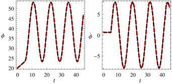
Figure 1: Periodic acceleration and deceleration of a Schlögl front realized by multiplicative control. Left: The numerically obtained front position (red dashed line) is in excellent agreement with the protocol of motion $\phi\left(t\right)=B_{0}+A\sin\left(2\pi t/T+B_{1}\right)$ (black solid line). $B_{0/1}$ are determined by $\phi\left(t_{0}\right)=\phi_{0},\,\dot{\phi}\left(t_{0}\right)=c$ so that the protocol is smooth at $t=t_{0}$. Right figure shows velocities. See S1 in supplement for a movie.

$$\mathbf{u}_{d}\left(x,t\right) =\mathbf{U}_{c}\left(x-\phi\left(t\right)\right).$$ (9)

The coupling matrix $\mathcal{G}$ depends upon the ability to control system parameters in a spatio-temporal way. In general, if $\mathbf{R}\left(\mathbf{u};\mathbf{p}\right)$ depends on the controllable parameters $\mathbf{p}$, we substitute $\mathbf{p}\rightarrow\mathbf{p}+\epsilon\mathbf{f}$, expand in $\epsilon$, and define the coupling matrix by ${\mathcal{G}\left(\mathbf{u}\right)=\partial\mathbf{R}\left(\mathbf{u};\mathbf{p}\right)/\partial\mathbf{p}}$. As an example, we consider an autocatalytic chemical reaction mechanism proposed by Schlögl ${A_{1}+2X\overset{k_{1}^{+}}{\underset{k_{1}^{-}}{\rightleftharpoons}}3X,\,X\overset{k_{2}^{+}}{\underset{k_{2}^{-}}{\rightleftharpoons}}A_{2}}$ Schlogl1972crm . Under the assumption that the concentrations $c_{1/2}=\left[A_{1/2}\right]$ of the chemical species $A_{1/2}$ are kept constant in space and time, a cubic reaction function ${R\left(u\right)=k_{1}^{+}c_{1}u{}^{2}-k_{1}^{-}u{}^{3}-k_{2}^{+}u+k_{2}^{-}c_{2}}$ dictates the time evolution of the concentration $u=\left[X\right]$. We assume that the concentrations $c_{1/2}$ can be controlled spatio-temporally, i.e., $c_{1/2}\rightarrow c_{1/2}+\epsilon f\left(x,t\right)$. Control by $c_{2}$ will be additive with $\mathcal{G}\left(u\right)=k_{2}^{-}$, while for control via $c_{1}$ the spatio-temporal forcing couples multiplicatively to the RD kinetics and $\mathcal{G}\left(u\right)=k_{1}^{+}u^{2}$. A different example for position control, realized experimentally in wolff2003gentle , exploits the dependency of the rate coefficients $k_{1/2}^{\pm}$ on temperature $T$ according to the Arrhenius law $k\sim e^{-E/\left(k_{B}T\right)}$. Substituting $T\rightarrow T+\epsilon f\left(x,t\right)$ and expansion in $\epsilon$ yields the coupling function $\mathcal{G}\left(u\right)$.

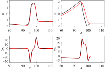
Figure 2: Snapshot of position control of a FHN pulse with an invertible coupling matrix $\mathcal{G}$ taken from movie S2 in supplement . Results by analytical control (black solid) agree very well with results obtained by optimal control (red dashed). Clockwise from top left: activator $u$, inhibitor $v$, controls $f{}_{u},\,f_{v}$.

In the bistable parameter regime, the unperturbed Schlögl model has an analytically known traveling front solution $U_{c}$ connecting the stable and the metastable homogeneous steady state as $x\rightarrow\pm\infty$ Schlogl1972crm . Suppose we want to move the front periodically back and forth in a sinusoidal manner via a spatio-temporal control of parameter $c_{1}$. Fig. 1 left shows that the numerically obtained front position follows the protocol very closely. The maximum enforced front velocity, $\max_{t}\dot{\phi}\left(t\right)=7.854$, is much larger than the velocity $c=0.662$ of the uncontrolled front, compare Fig. 1 right.

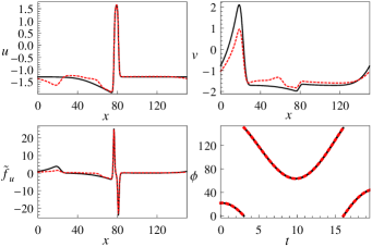
Figure 3: Snapshot of position control of a FHN pulse with a non-invertible coupling matrix $\mathcal{G}$. The control $\tilde{f}_{u}$ (bottom left) acts solely on the activator equation. The controlled inhibitor pulse profile (top right) is much more deformed than the activator pulse profile (top left). Shown are results of optimal (red dashed) and analytical control (black solid). Bottom right: Analytical protocol (black solid) and numerically obtained position over time data for the maximum activator value of the controlled RDS (red dashed). See movie S3 supplement .

Now we apply position control to the stable traveling pulse solution of FitzHugh-Nagumo (FHN) equations

$$\partial_{t}u= D_{u}\partial_{x}^{2}u+f_{1}\left(u\right)-v+\epsilon\left(\mathcal{G}_{11}f_{u}+\mathcal{G}_{12}f_{v}\right),$$ (10)

$$\partial_{t}v= D_{v}\partial_{x}^{2}v+\tilde{\epsilon}\left(u-\delta\right)-\tilde{\epsilon}\gamma v+\epsilon\left(\mathcal{G}_{21}f_{u}+\mathcal{G}_{22}f_{v}\right),$$

where ${f_{1}=3u-u^{3}}$ and $\mathcal{G}_{ij}$ denote the components of the coupling matrix $\mathcal{G}$. As an example, we consider an accelerating protocol $\phi\left(t\right)=ct\left(1+t/4\right)$. We assume that two additive parameters can be controlled independently. For the choice ${\mathcal{G}=\small\left(\begin{array}[]{cc}1&0\\ 1/2&1\end{array}\right)}$, $\mathcal{G}$ is invertible. The obtained control function as well as the controlled pulse profile are close to the corresponding results obtained by an optimal control, see Fig. 2.
If the coupling matrix $\mathcal{G}$ is not invertible, Eq. (7) for the control cannot be used. Because the inhibitor kinetics is linear in $v$, Eq. (10) can be written as a single nonlinear integro-differential equation (IDE) for the activator $u$

$$\partial_{t}u =D_{u}\partial_{x}^{2}u+f_{1}\left(u\right)-\mathcal{K}\left(\tilde{\epsilon}\left(u-\delta\right)+\epsilon f_{v}\right)-\mathcal{K}_{0}v_{0}+\epsilon f_{u}.$$ (11)

$\mathcal{K}$ and $\mathcal{K}_{0}$ are integral operators, involving Green’s function, of the inhomogeneous linear PDE for the inhibitor $v$ with initial condition $v\left(x,t_{0}\right)=v_{0}\left(x\right)$

$$\partial_{t}v-D_{v}\partial_{x}^{2}v+\tilde{\epsilon}\gamma v =\tilde{\epsilon}\left(u-\delta\right)+\epsilon f_{v}.$$ (12)

We contrast Eq. (11) with the equation obtained from Eq. (11) by substituting $f_{u}\rightarrow\tilde{f}_{u},\,f_{v}\rightarrow 0$. Comparing the control terms yields the control $\tilde{f}_{u}$ acting solely on the activator equation,

$$\tilde{f}_{u} =-\mathcal{K}f_{v}+f_{u},$$ (13)

were $f_{u}$ and $f_{v}$ are given by Eq. (7) with $\mathcal{G}\equiv 1$. We apply the control $\tilde{f}_{u}$ with a sinusoidal protocol to a FHN pulse. The activator’s maximum follows the protocol closely, see bottom right of Fig. 3. Comparing the result for $\tilde{f}_{u}$, Eq. (13), with an optimal control result reveals good overall agreement (bottom left of Fig. 3). However, for both control methods the inhibitor profile (top right) is largely deformed although the activator profile remains comparably unaffected (top left). Reduction of the RD equations to a single IDE and thereby derivation of a control is possible for, but not restricted to, all models of the form supplement

$$\partial_{t}u =D_{u}\partial_{x}^{2}u+f\left(u,v_{2},\dots,v_{n}\right)+\epsilon f_{u},$$ (14)

$$\partial_{t}v_{i} =D_{i}\partial_{x}^{2}v_{i}+h_{i}\left(u\right)v_{i}+g_{i}\left(u\right)+\epsilon f_{i},\,i\in\left\{2,\dots,n\right\}.$$

This class includes Hodgkin-Huxley type models (with ${D_{i}=0}$) for the action potential propagation in neuronal and cardiac tissue murray1993mathematical . The modified Oregonator model describing the light-sensitive BZ reaction krug1990analysis is not of the form Eq. (14) but can nevertheless be written as a single IDE. We present position control of chemical concentration waves in the photosensitive BZ reaction applying actinic light of space-time dependent intensity to the reaction in the supplemental material S6 supplement .
In many experiments, a stationary control $f\left(x\right)$ is much less demanding to realize than a spatio-temporal control $f\left(x,t\right)$. For single component RD systems, we can formulate a Fredholm integral equation of the first kind for $f\left(x\right)$

$$g\left(\phi\right)=cK_{c}-\frac{K_{c}}{T^{\prime}\left(\phi\right)} =\int_{-\infty}^{\infty}dxK\left(\phi-x\right)f\left(x\right),$$ (15)

with kernel ${K\left(x\right)=e^{-cx/D}U_{c}^{\prime}\left(-x\right)\mathcal{G}\left(U_{c}\left(-x\right)\right)}$ and inhomogeneity $g$. We introduced the inverse function ${T=\phi^{-1}}$ and used the general expression for the adjoint Goldstone mode for single component systems, ${W^{\dagger}\left(x\right)=e^{cx/D}U_{c}^{\prime}\left(x\right)}$. Eq. (15) can be solved with the help of the convolution theorem for the two-sided Laplace transform, see supplement .
As an example, we choose a protocol which drives the propagation velocity to zero according to

$$\dot{\phi}\left(t\right) =\dfrac{c}{2}\left(1+\tanh\left(k\left(t_{1}-t\right)\right)\right),\;t_{1}>t_{0},\,k>0.$$ (16)

In the limit $k\rightarrow\infty$, this protocol would stop the front instantaneously at time $t=t_{1}$ because $\lim_{k\rightarrow\infty}\dot{\phi}\left(t\right)=c\Theta\left(t_{1}-t\right)$, where $\Theta$ represents the Heaviside Theta function. For the inhomogeneity $g$ we find

$$g\left(\phi\right) =K_{c}\frac{c\exp\left(\frac{2k}{c}\left(ct_{0}+\phi-\phi_{0}\right)\right)}{e^{2kt_{0}}+e^{2kt_{1}}}.$$ (17)

An additive control with $\mathcal{G}\left(u\right)=1$ is assumed.
We consider a rescaled Schlögl model with reaction function $R\left(u\right)=-u\left(u-a\right)\left(u-1\right)$. The front solution is given as $U_{c}\left(\xi\right)=1/\left(1+\exp\left(\xi/\sqrt{2}\right)\right)$ with propagation velocity $c=\left(1-2a\right)/\sqrt{2}$ for $D=1$. The region of convergence of the Laplace transforms of kernel $K$ and inhomogeneity $g$ determines the range of allowed values for $k$ as $0<k<c\left(1/\sqrt{2}-c\right)/2=k_{\text{max}}$. This amounts to a minimum acceleration (or maximum deceleration) at time $t=t_{1}$ equal to

$$\ddot{\phi}\left(t_{1}\right)= -\dfrac{c}{2}k>-\left(\dfrac{c}{2}\right)^{2}\left(\dfrac{1}{\sqrt{2}}-c\right),$$ (18)

which can be realized under this control given explicitly by

$$f\left(x\right) =-\frac{K_{c}c^{2}\sin\left(\frac{\sqrt{2}\pi}{c}\left(c^{2}+2k\right)\right)e^{\frac{2k}{c}\left(x-\phi_{0}\right)}}{\sqrt{2}\pi\left(1+e^{2k\left(t_{1}-t_{0}\right)}\right)\left(c^{2}+2k\right)}.$$ (19)

The divergence for $x\rightarrow\infty$ can be circumvented by cutting off $f$ in such a way that ${R\left(u\right)+\epsilon f\left(x\right)=0}$ locally keeps three different real roots, meaning that bistability is preserved at every point in space. A more systematic approach to prevent divergence of $f\left(x\right)$ would be to consider the Fredholm integral equation Eq. (15) supplemented with inequality constraints ${f_{\text{min}}\leq f\leq f_{\text{max}}}$ for the control function.
Under the control Eq. (19), the velocity of the numerical solution first follows the protocol velocity closely, see right inset of Fig. 4. Deviations arise when the transition region of the front enters the domain with large absolute values of the control. These velocity deviations accumulate to a difference in the position at which the front is stopped. The front profile is slightly deformed in the region where the control is large because the solution Eq. (19) is not proportional to the Goldstone mode, see left inset in Fig. 4.

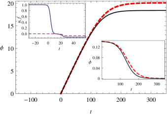
Figure 4: Deceleration of a Schlögl front by an additive stationary control. Red dashed line is the result of numerical simulations, black solid line is the pre-given protocol. Shown are the position $\phi$ and the velocity $\dot{\phi}$ (right inset). The front profile (blue solid line) is slightly deformed in the region where the control (purple dotted line) is large, see left inset. Compare also S8 in supplement .

In conclusion, we have demonstrated that the proposed method is well-suited to control the position of traveling fronts and pulses in RD systems according to a pre-given protocol of motion $\phi\left(t\right)$ while preserving the profile $\mathbf{U}_{c}$ of the uncontrolled wave. To determine the control functions $\mathbf{f}$, primarily the profile of the uncontrolled TW must be known. In the majority of cases this profile can be obtained only numerically or experimentally. Especially in the latter case measurements must be sufficiently accurate to determine the Goldstone mode $\mathbf{U}_{c}^{\prime}\left(x\right)$. Additionally, the propagation velocity $c$ and the invertible coupling matrix $\mathcal{G}$ are needed. For stationary control Eq. (15) additionally the value of the diffusion coefficient $D$ is required. Remarkably, the knowledge of the nonlinearity $\mathbf{R}\left(\mathbf{u}\right)$ is not necessary for the calculation of the control functions. This makes the method powerful for applications where details of the underlying kinetics $\mathbf{R}\left(\mathbf{u}\right)$ are only approximately known but the wave profile can be measured with required accuracy. Examples do not not only include chemical and biological applications but also population dynamics and spreading diseases murray1993mathematical . Because TW profiles $\mathbf{U}_{c}\left(x\right)$ decay exponentially fast as $x\rightarrow\pm\infty$, the control Eq. (7) is usually localized. If the coupling matrix $\mathcal{G}$ is not invertible and the RD system is of the form Eq. (14), a control function can still be derived, however, more detailed knowledge of the reaction kinetics is required, see Eq. (13). In all cases considered the spatio-temporal control Eq. (7) was found to be close to an optimal control. We emphasize that in contrast to our method, computation of an optimal control requires full knowledge of the reaction kinetics and computationally expensive algorithms.
An important issue is reliability of the proposed controls. Large control amplitudes $A=c-\dot{\phi}$, Eq. (7), sometimes destroy the TW and can lead to the spontaneous generation of waves, as was also observed in wolff2003gentle . We demonstrate such behavior in the supplemental material, see S7 in supplement . In general, the range of protocol velocities $\dot{\phi}$ achievable by the proposed control method depends on the reaction kinetics, the parameter values and higher order derivatives of $\dot{\phi}$. A necessary condition for the EOM Eq. (4) to be valid is the existence of a spectral gap for the operator $\mathcal{L}$, Eq. (3). For the Fisher equation, we found a successful position control despite there is no spectral gap. An additive control attempting to stop the front leads to a front profile growing indefinitely to $-\infty$, while a multiplicatively coupled control accomplishes this task without significantly deforming the front profile, see S4 and S5 in supplement .
Generalizing the proposed method to higher spatial dimensions allows a precise control of shapes of RD patterns. These findings as well as extensions to conservative nonlinear systems and results regarding the stability of the control method will be published elsewhere.

- (1) A. Mikhailov and K. Showalter, Phys. Rep. 425, 79 (2006)
- (2) V. Vanag and I. Epstein, Chaos 18, 026107 (2008)
- (3) E. Mihaliuk, T. Sakurai, F. Chirila, and K. Showalter, Phys. Rev. E 65, 065602 (2002)
- (4) V. S. Zykov, G. Bordiougov, H. Brandtstädter, I. Gerdes, and H. Engel, Phys. Rev. Lett. 92, 018304 (2004)
- (5) V. Zykov and H. Engel, Physica D 199, 243 (2004)
- (6) T. Sakurai, E. Mihaliuk, F. Chirila, and K. Showalter, Science 296, 2009 (2002)
- (7) J. Wolff, A. G. Papathanasiou, H. H. Rotermund, G. Ertl, X. Li, and I. G. Kevrekidis, Phys. Rev. Lett. 90, 018302 (2003)
- (8) J. Wolff, A. G. Papathanasiou, I. G. Kevrekidis, H. H. Rotermund, and G. Ertl, Science 294, 134 (2001)
- (9) P. Kevrekidis, I. Kevrekidis, B. Malomed, H. Nistazakis, and D. Frantzeskakis, Phys. Scr. 69, 451 (2004)
- (10) H. Nistazakis, P. Kevrekidis, B. Malomed, D. Frantzeskakis, and A. Bishop, Phys. Rev. E 66, 015601 (2002)
- (11) B. Malomed, D. Frantzeskakis, H. Nistazakis, A. Yannacopoulos, and P. Kevrekidis, Phys. Lett. A 295, 267 (2002)
- (12) F. Tröltzsch, Optimal control of partial differential equations (American Mathematical Society, Providence, 2010)
- (13) J. Nocedal and S. J. Wright, Numerical optimization (Springer New York, 1999)
- (14) K. Theißen, Ph.D. thesis, Westfälische Wilhelms-Universität, Münster (2006)
- (15) R. Buchholz, H. Engel, E. Kammann, and F. Tröltzsch, Comput. Optim. Appl. 56, 153 (2013)
- (16) See Supplemental Material at [URL will be inserted by publisher] for additional derivations, movies, and information on the parameter values chosen for numerical simulations.
- (17) C. M. Bender and S. A. Orszag, Advanced mathematical methods for scientists and engineers (McGraw-Hill, New York, 1978)
- (18) J. Löber, M. Bär, and H. Engel, Phys. Rev. E 86, 066210 (2012)
- (19) L. Schimansky-Geier, A. S. Mikhailov, and W. Ebeling, Ann. Phys. (Leipzig) 495, 277 (1983)
- (20) A. Engel, Phys. Lett. A 113, 139 (1985)
- (21) A. Engel and W. Ebeling, Phys. Lett. A 122, 20 (1987)
- (22) A. Kulka, M. Bode, and H. Purwins, Phys. Lett. A 203, 33 (1995)
- (23) M. Bode, Physica D 106, 270 (1997)
- (24) A. Pikovsky, M. Rosenblum, and J. Kurths, Synchronization: a universal concept in nonlinear sciences (Cambridge University Press, Cambridge, 2003)
- (25) J. Yang, Nonlinear waves in integrable and non-integrable systems (SIAM, Philadelphia, 2011)
- (26) F. Schlögl, Z. Phys. A 253, 147 (1972)
- (27) J. D. Murray, Mathematical biology, Vol. 3 (Springer-Verlag, Berlin, 1993)
- (28) H. J. Krug, L. Pohlmann, and L. Kuhnert, J. Phys. Chem. 94, 4862 (1990)