Trapping Electromagnetic Solitons in Cylinders

Abstract

Electromagnetic waves, in vacuum or dielectrics, can be confined in unbounded cylinders in such a way that they turn around the main axis. For particular choices of the cylinder’s section, interesting stationary configurations may be assumed. By refining some results obtained in previous papers, additional more complex situations are examined here. For such peculiar guided waves an explicit expression is given in terms of Bessel’s functions. Possible applications are in the development of whispering gallery resonators.

Dipartimento di Fisica, Informatica e Matematica

Università di Modena e Reggio Emilia

Via Campi 213/B, 41125 Modena (Italy)

daniele.funaro@unimore.it

Keywords: electromagnetism, whispering gallery modes, Bessel functions.

PACS: 41.20.Jb, 02.30.Gp, 02.60.Cb, 42.60.Da.

1 Introduction

The classical equations of electromagnetism allow for solutions confined in ring-shaped domains. In vacuum, this is made possible by the orthogonality of the electric and magnetic fields (${\bf E}$ and ${\bf B}$) and by the enforcement of the two divergence-free conditions (${\rm div}{\bf E}=0$ and ${\rm div}{\bf B}=0$). In fact, if the lines of force are closed and orthogonal, a toroid is a natural environment to set up the initial conditions, that successively evolve according to:

$$\frac{\partial{\bf E}}{\partial t}~{}=~{}c^{2}{\rm curl}{\bf B}\hskip 42.67912pt\frac{\partial{\bf B}}{\partial t}~{}=~{}-{\rm curl}{\bf E}$$ (1)

where $c$ denotes the speed of light. The above time-dependent equations are easily put in relation with the vector wave equation and its corresponding eigenmodes.

The search for electromagnetic waves trapped in a toroid poses interesting mathematical questions. Numerical computations show a variety of solutions, whose dynamics depends on the section’s shape. The behavior is strikingly similar to that of a non-viscous fluid confined in a vortex ring, but with additional intrinsic constraints.

Explicit full solutions in terms of Bessel functions are available in the case of cylinders, where the magnetic field oscillates parallel to the axis and the electric field lays on the circular sections. The configuration recalls that of a train of solitons smoothly circulating inside a 2D rounded cavity. As documented in [2], thin rings with large diameter and circular section can be well approximated by the above mentioned solutions.

For more compact rings the use of numerical simulations is a necessity. By the way, not all the shapes are workable. Indeed, only a restricted range of sections are compatible with the electromagnetic constraints. Thus, the solution process must be implemented together with a sort of shape-detection algorithm (see [2]).

Extensions of previous results (briefly recalled in the next section) are here obtained for electromagnetic waves trapped in unbounded cylinders where, the rotation around the axis is combined with a radial oscillation. Here we assume that the section is an annulus, so that the corresponding domain is a hollow cylinder. Having in mind the vector wave equation, the study is connected to the search of eigenfunctions of the Laplace operator in such a way that the dimension of the corresponding eigenspace is equal to four. As we will see, this analysis leads to the study of specific properties of Bessel’s functions.

2 Electromagnetic waves turning around an axis

We assume that $k\geq 1$ is an integer number. We recall that the $k$-th Bessel’s functions, of the first and the second kinds respectively, are independent solutions to the same eigenvalue problem ($r>0$):

$$J_{k}^{\prime\prime}(\omega r)~{}+~{}\frac{J_{k}^{\prime}(\omega r)}{r}~{}-~{}\frac{k^{2}J_{k}(\omega r)}{r^{2}}~{}=~{}-\omega^{2}J_{k}(\omega r)$$ (2)

$$Y_{k}^{\prime\prime}(\omega r)~{}+~{}\frac{Y_{k}^{\prime}(\omega r)}{r}~{}-~{}\frac{k^{2}Y_{k}(\omega r)}{r^{2}}~{}=~{}-\omega^{2}Y_{k}(\omega r)$$ (3)

for a given parameter $\omega$. We also recall that $J_{k}$ tends to zero for $r\rightarrow 0$, while $Y_{k}$ is unbounded in the neighborhood of $r=0$ (see, e.g., [9]).

Solutions of the entire set of Maxwell’s equations are obtained in cylindrical coordinates $(r,z,\phi)$ as follows (see [3], [4]):

$${\bf E}=\left(\frac{kf(\omega r)}{\omega r}\cos(c\omega t-k\phi),~{}~{}0,~{}f^{\prime}(\omega r)\sin(c\omega t-k\phi)\right)$$

$${\bf B}~{}=~{}\frac{1}{c}\Big{(}0,~{}f(\omega r)\cos(c\omega t-k\phi),~{}~{}0\Big{)}$$ (4)

where $f$ is a linear combination of $J_{k}$ and $Y_{k}$. The magnetic field is parallel to the cylinder’s axis and the electric field belongs to the plane $(r,\phi)$. Bounded solutions are possible in two cases: the domain is such that $r\geq R_{m}>0$ for some given $R_{m}$ (see for instance the second picture in Fig. 1); the function $f$ is just a multiple of $J_{k}$, thus $r=0$ may be included in the domain (see for instance the first picture in Fig. 1).

The displacement of the electric field at a given time is shown in Fig. 1 for $k=1$. During time evolution, the electromagnetic wave rigidly rotates around the central point. Two examples are taken into account. In the left picture, the domain is the circle $0\leq r\leq R_{M}$, where $R_{M}$ is the first zero of $J_{1}$, which takes approximately the value 3.832. In this way, at the boundary, both the magnetic field and the radial component of the electric field are zero. In the right picture, we have the annular region $R_{m}=1\leq r\leq R_{M}$. The outer diameter is now chosen in such a way that the electric field is orthogonal to the boundary (perfect conductivity).

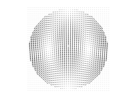
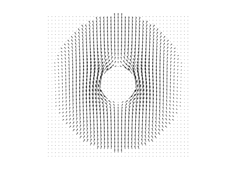
Figure 1: Displacement of the electric field at fixed time obtained from the expression in (4) subject to different kinds of boundary constraints. The sizes of the domains are not arbitrary, but strictly related to the frequency of rotation as well as boundary conditions. The magnetic field is orthogonal to the page.

Once the frequency of rotation (depending on $c\omega$) is fixed and the type of boundary conditions decided, the size of the domain is automatically constrained. This means that there are few domains allowing for the creation of these waves. If the proper size is not respected, the wave will not follow a stationary motion, i.e., it does not complete the cycle preserving the phase. The conditions that permit such a guided behavior depend on the eigenvalues of the Laplace operator on the domain. If the shape is such that some eigenvalues have multiplicity higher than one, then the construction of such rotating solitary waves is possible (we show later the determination process). An analysis of spherical vortices has been provided in [2], exactly with the purpose of detecting domains where two independent eigenfunctions are related to the same eigenvalue. In this paper, we stay for simplicity in the case of the cylinder by analyzing the peculiar case where four independent eigenfunctions share the same eigenvalue. The evolution in a thin toroid can be approximated, with a rather good level of accuracy, starting from the cylinder’s version; this extension however is not going to be studied here.

3 A more involved evolution

We would like to analyze the situation in which the multiplicity of one of the eigenvalues of the Laplace operator, on a certain annular domain, is equal to four. This will allow us to build more complex electromagnetic waves turning around an axis. We will need to play with both the functions $J_{k}$ and $Y_{k}$, therefore we have to stay away from the point $r=0$ (recall that $Y_{k}$ is singular there). From now on we assume that $R_{m}=1\leq r\leq R_{M}$, where the major diameter $R_{M}$ has to be properly determined. Of course, if $R_{m}$ is modified the entire setting scales accordingly due to the linearity of Maxwell’s equations.

We impose Dirichlet boundary conditions on both boundaries (the inner and the outer circumferences), though other conditions may be considered. Taking Dirichlet conditions in the inner part involves working with the function:

$$f_{n}(r)~{}=~{}J_{n}(\lambda r)Y_{n}(\lambda)~{}-~{}Y_{n}(\lambda r)J_{n}(\lambda)$$ (5)

where $\lambda>0$ is a parameter. Of course, we have $f_{n}(1)=0$, $\forall n$ and $\forall\lambda$.

Now, we would like to have:

$$\begin{cases}f_{n}(R_{M})~{}~{}=~{}0\cr f_{m}(R_{M})~{}=~{}0\end{cases}~{}~{}~{}~{}~{}~{}~{}~{}~{}~{}~{}~{}~{}m\not=n$$ (6)

which is a nonlinear problem leading to the detection of $R_{M}$ and $\lambda$. This means that, once the diameter of the inner circumference has been fixed, the frequency of the evolving wave and the magnitude of the entire domain are going to be uniquely determined by (6). Not necessarily such a problem has solution. However, with the help of numerical tests, we were able to establish some facts.

Here below we report some of the conclusions of our analysis:

$$m=1,~{}n=2:~{}{\rm no~{}values~{}of}~{}R_{M}~{}{\rm and}~{}\lambda~{}{\rm were~{}found}$$

$$m=1,~{}n=3:~{}{\rm no~{}values~{}of}~{}R_{M}~{}{\rm and}~{}\lambda~{}{\rm were~{}found}$$

$$m=1,~{}n=4:~{}~{}~{}R_{M}=7.0927~{}~{}~{}{\rm for}~{}\lambda=1.0698$$

$$m=1,~{}n=5:~{}~{}~{}R_{M}=3.6761~{}~{}~{}{\rm for}~{}\lambda=2.3871$$

$$m=1,~{}n=6:~{}~{}~{}R_{M}=2.7603~{}~{}~{}{\rm for}~{}\lambda=3.6054$$

$$m=2,~{}n=3:~{}{\rm no~{}values~{}of}~{}R_{M}~{}{\rm and}~{}\lambda~{}{\rm were~{}found}$$

$$m=2,~{}n=4:~{}{\rm no~{}values~{}of}~{}R_{M}~{}{\rm and}~{}\lambda~{}{\rm were~{}found}$$

$$m=2,~{}n=5:~{}~{}~{}R_{M}=5.1500~{}~{}~{}{\rm for}~{}\lambda=1.7032$$

Let us better examine a specific situation ($m=1$, $n=4$). According to Fig. 2, both functions $f_{1}$ and $f_{4}$ are zero for $r=R_{m}=1$ and $R_{M}\approx 7.0927$. Thus, by imposing the same boundary constraints, we are able to find out two branches of vector solutions of the type given in (4) ($k=m$ and $k=n$ respectively) related to the same frequency of rotation. These are generated by magnetic fields whose intensity is given by the level lines of Fig. 3.

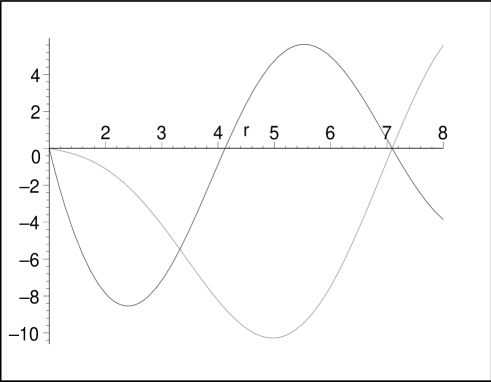
Figure 2: Plots of $f_{1}$ and $f_{4}$ for $\lambda\approx 1.0699$. In this case both the functions vanish at $r=1$ and $r\approx 7.0927$.

Successively, starting from $\lambda$, we can build general solutions of the form:

$$w_{1}\sin(c\sqrt{\lambda}~{}t-\phi_{0})+w_{2}\sin(c\sqrt{\lambda}~{}t)+w_{3}\cos(c\sqrt{\lambda}~{}t-\phi_{0})+w_{4}\cos(c\sqrt{\lambda}~{}t)$$ (7)

The function $w_{j}$, $j=1,2,3,4$, are schematically reported in Fig. 4. In particular, $w_{1}$ and $w_{3}$ are as shown in the first picture of Fig. 3, but with a difference of phase of 90 degrees. Combining $w_{1}$ and $w_{3}$ we can obtain the electromagnetic fields according to the expression (4) for $k=1$. The other two functions, $w_{2}$ and $w_{4}$, are as shown in the second picture of Fig. 3 and differ for an angle of 22.5 degrees. They also lead to (4) (this time with $k=4$). The phase lag $\phi_{0}$ is arbitrarily given.

It is just a direct computation verifying that the expression provided in (7) solves the wave equation in vacuum. In fact, the second derivative in time produces the multiplicative factor $-c^{2}\lambda$, while the application of the Laplace operator is equivalent to a multiplication by $-\lambda=-\omega^{2}$ (see (2) and (3)).

In Fig. 5, one can see, at different time steps, the evolution of (7) for $\phi_{0}=0$. Only half cycle is displayed. From the last picture the sequence restarts from the beginning with the color interchanged. An animation is available in [5]. The effect vaguely recalls the juggling of three clubs.

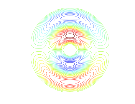
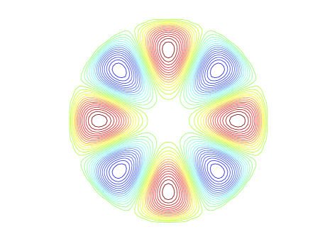
Figure 3: Plots of two independent eigenfunctions of the Laplace operator with homogeneous Dirichlet boundary conditions on an annular domain. Despite the fact that they look totally different, the domain has been dimensioned in such a way the corresponding eigenvalues are the same.

    

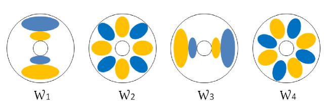
Figure 4: Schematic representation of four independent eigenfunctions on the annular domain having the same eigenvalue.

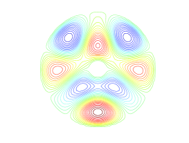
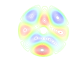
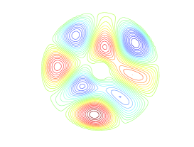
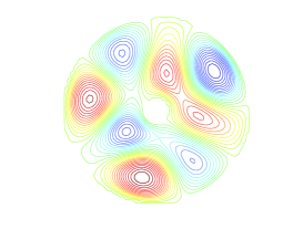
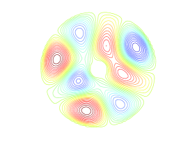
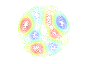
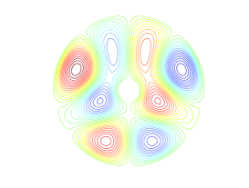
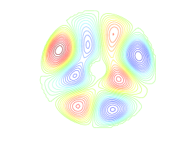
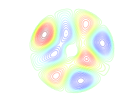
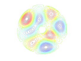
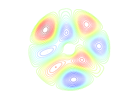
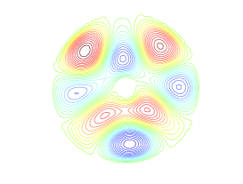
Figure 5: Evolution at different times of a linear combination of eigenfunctions corresponding to the same eigenvalue. The two eigenfunctions of Fig. 3 merge and rotate with a periodic behavior. The frequency is uniquely established by the global size of the domain.

4 Conclusions

From the theoretical viewpoint, Maxwell’s equations allow for special solutions trapped inside an infinite cylinder or, more or less equivalently, in a toroid. The study here developed in vacuum reveals original configurations and may help for instance in the analysis of confined plasma (see, e.g., [6]). Other applications may be found in the field of the so called whispering gallery resonators. Waves trapped in these cavities are smoothly guided to circulate around by continuous reflection returning at the origin with the initial phase. Spherical, cylindrical and ring-shaped whispering galleries are commonly produced for a broad range of industrial applications. Typical areas of interest are in fiber telecommunications or biosensing. The literature is very rich. We just mention a couple of non extremely specialized publications: [7], [8].

References

- [1]
- [2] Chinosi C., Della Croce L., Funaro D., Rotating electromagnetic waves in toroid-shaped regions, International Journal of Modern Physics C, 21-1 (2010), pp.11-32.
- [3] Funaro D., Electromagnetism and the Structure of Matter, World Scientific, Singapore, 2008.
- [4] Funaro D., From Photons to Atoms - The Electromagnetic Nature of Matter, arXiv:1206.3110, 2012.
- [5] Funaro D., http://cdm.unimo.it/home/matematica/funaro.daniele/results.htm.
- [6] Hazeltine R.D., Meiss J.D., Plasma Confinement, Dover Pub., Mineola NY, 2003.
- [7] Oraevsky A.N., Whispering-gallery waves, Quantum Electronics, 32 (2002), pp. 377-400.
- [8] Snyder A., Love J., Optical Waveguide Theory, Kluwer Academic Publisher, Norwell MA, 1983.
- [9] Watson G.N., A Treatise on the Theory of Bessel Functions, Cambridge Univ. Press, 1944.