Single vector-like top partner production in the Left-Right Twin Higgs model at TeV energy $e\gamma$ colliders

Abstract

The left-right twin Higgs model contains a new vector-like heavy top quark, which mixes with the SM-like top quark. In this work, we studied the single vector-like top partner production via process $e^{-}\gamma\rightarrow\nu_{e}\bar{T}b$ at the International Linear Collider. We calculated the production cross section at tree level and displayed the relevant differential distributions. The result shows that there will be 125 events produced each year with $\sqrt{s}$=$2$TeV and the integrated luminosity $\mathcal{L}_{int}\simeq 500fb^{-1}$, and the b-quark tagging and the relevant missing energy $\not\!\!\!E_{T}$ cut will be helpful to detect this new effect.

I Introduction

The top quark was first observed at Ferminlab Tevatron in 1995 top and is by far the heaviest elementary fermion. Due to the large mass, the top quark decays rapidly before forming any hadronic bound state. Furthermore, the top quark has many properties different from other quarks, so it occupies a special position in the standard model(SM) and is often speculated to be sensitive to the new physics. For these reasons, probing the properties of the top quark is always one of the forefront topics at the various high energy collider.

The twin Higgs theories use a discrete symmetry in combination with an approximate global symmetry to stabilize the Higgs mass. This mechanism can be implemented in left-right models with the discrete left-right symmetry lrhiggs . In the left-right twin Higgs(LRTH) model, a vector-like top quark is introduced in order to give the top quark a mass of the order of electroweak scale. There is mixing between the SM-like top quark and the heavy top quark so that the top quark couplings can be modified. At the LHC, a single vector-like top quark can be produced dominantly via s-channel or t-channel $W$ or $W_{H}$ exchange, while the production of the vector-like top quark pair can be produced dominantly from gluon exchange. The productions and decays of the vector-like top quark at the LHC have been described in detail in Refs.heavy top . If this effect can be detected, it will be the most compelling evidence of the new physics.

Duo to the complicated QCD background, the measurement precision of the LHC is limited. By contrast, the background of the International Linear Collider(ILC) is very clean so that it will allow unique opportunities to study the properties and interactions of the SM top quark and vector-like top quark. Besides the $e^{+}e^{-}$ collider mode, the $\gamma\gamma$ or $e\gamma$ collider mode can be realized by the backward Compton scattering at the ILCILC . The search for deviations from the SM couplings in single top quark production has become one of the main focus in the on-going and forthcoming collider experimentssingle top . In this paper, we study the process $e^{-}\gamma\rightarrow\nu_{e}\bar{T}b$, the results will be helpful to test the SM and the LRTH model.

This paper is organized as follows. In Sec.II we give a brief review of the LRTH model. In Sec.III we calculate the production cross section of the process $e^{-}\gamma\rightarrow\nu_{e}\bar{T}b$ and the differential distributions of several observables at the ILC. Finally, we give our conclusions and some comments in Sec.IV.

II A brief review of the LRTH model

The LRTH model was first proposed in Ref.LRTH and some phenomenological analye and the Feynman rules have been studied in Ref.ph-LRTH . In this section we will briefly review the essential features of the LRTH model related to our work.

In the LRTH model, the global symmetry is $U(4)\times U(4)$, with a diagonal subgroup $SU(2)_{L}\times SU(2)_{R}\times U(1)_{B-L}$ gauged. Two Higgs fields, $H$ and $\hat{H}$, are introduced and each transforms as $(\textbf{4},\textbf{1})$ and $(\textbf{1},\textbf{4})$ respectively under the global symmetry. They are written as

$$H=\left(\begin{array}[]{c}H_{L}\\ H_{R}\\ \end{array}\right)\,,~{}~{}~{}~{}~{}~{}~{}~{}~{}~{}~{}~{}~{}~{}\hat{H}=\left(\begin{array}[]{c}\hat{H}_{L}\\ \hat{H}_{R}\\ \end{array}\right)\,,$$ (5)

where $H_{L,R}$ and $\hat{H}_{L,R}$ are two component objects which are charged under the $SU(2)_{L}\times SU(2)_{R}\times U(1)_{B-L}$ as

$$H_{L}{\rm\ and\ }\hat{H}_{L}:(\textbf{2},\textbf{1},1),~{}~{}~{}~{}~{}~{}~{}~{}H_{R}{\rm\ and\ }\hat{H}_{R}:(\textbf{1},\textbf{2},1).$$ (6)

After Higgses develop vacuum expectation values (vevs) as $\langle H\rangle=(0,0,0,f)$ and $\langle\hat{H}\rangle=(0,0,0,\hat{f})$, which break the $U(4)\times U(4)$ global symmetry as well as the gauge symmetry ${\rm SU}(2)_{R}\times{\rm U}(1)_{B-L}$ down to the SM ${\rm U}(1)_{Y}$.

After the electroweak breaking of $SU(2)_{L}\times U(1)_{Y}$, three Goldstone bosons are eaten by the massive gauge bosons $W^{\pm}$ and $Z$ in the SM, their masses can be given by

$$M_{W}^{2} = \frac{1}{2}g_{2}^{2}f^{2}\sin^{2}x,$$ (7)

$$M_{Z}^{2} = \frac{g_{2}^{2}+g_{Y}^{2}}{g_{2}^{2}}\frac{2M_{W}^{2}M_{W_{H}}^{2}}{M_{W}^{2}+M_{W_{H}}^{2}+\sqrt{(M_{W_{H}}^{2}-M_{W}^{2})^{2}+4\frac{g_{1}^{4}}{(g^{2}+g_{1}^{2})^{2}}M_{W_{H}}^{2}M_{W}^{2}}}$$ (8)

where $x=v/(\sqrt{2}f)$ and $v=246$GeV is the electroweak scale, $g_{Y}$ is the SM hypercharge coupling, $M_{W_{H}}$ is the $W_{H}^{\pm}$ mass, the values of $f$ and $\hat{f}$ will be bounded from below by electroweak precision measurements.

In order to give the top quark mass of the order of the electroweak scale, a pair of vector-like quarks $Q_{L}$ and $Q_{R}$ is introduced. The mass eigenstates, which contain one of the SM-like top quark $t$ and a heavy top partner $T$, are mixtures of the gauge eigenstates. Their masses are given by

$$m_{t}^{2}=\frac{1}{2}(M^{2}+y^{2}f^{2}-N_{t}),\hskip 14.22636ptM_{T}^{2}=\frac{1}{2}(M^{2}+y^{2}f^{2}+N_{t}),$$ (9)

where $N_{t}=\sqrt{(y^{2}f^{2}+M^{2})^{2}-y^{4}f^{4}\sin^{2}2x}$.

At the leading order, the mixing angles for the left-handed and right-handed fermions are

$$s_{L} \simeq \frac{M}{m_{T}}\sin x,$$ (10)

$$s_{R} \simeq \frac{M}{m_{T}}(1+\sin^{2}x),$$ (11)

where $M$ is the mass parameter essential to the mixing between the top quark $t$ and its partner $T$.

III Single vector-like top production via process $e^{-}\gamma\rightarrow\nu_{e}\bar{T}b$

Figure 1: Feynman diagrams of the process $e^{-}\gamma\rightarrow\nu_{e}\bar{T}b$ in the left-right twin Higgs model.

At a linear collider the single vector-like top quarks can be produced from the following two processes:

$$T:e^{+}\gamma\rightarrow\bar{\nu}_{e}T\bar{b},~{}~{}~{}~{}~{}~{}~{}~{}~{}\bar{T}:e^{-}\gamma\rightarrow\nu_{e}\bar{T}b$$ (12)

where the photon comes from the original incoming electron and positron, respectively. The relevant Feynman diagrams of the process $e^{-}\gamma\rightarrow\nu_{e}\bar{T}b$ in the LRTH model are shown in Fig.1.

The invariant production amplitudes of the process $e^{-}\gamma\rightarrow\nu_{e}\bar{T}b$ can be written as:

$$\mathcal{M}=\mathcal{M}_{a}+\mathcal{M}_{b}+\mathcal{M}_{c}+\mathcal{M}_{d}$$ (13)

with

$$M_{a} = \varepsilon_{\rho}(p_{2})\bar{u}(p_{3})V_{W\nu e}^{\mu}u(p_{1})\bar{u}(p_{5})V_{WTb}^{\alpha}v(p_{4})V_{WW\gamma}^{\nu\rho\beta}$$ (14)

$$\frac{-ig_{\mu\nu}}{(p_{1}-p_{3})^{2}-m_{W}^{2}}\frac{-ig_{\alpha\beta}}{(p_{4}+p_{5})^{2}-m_{W}^{2}}$$

$$M_{b} = \varepsilon_{\rho}(p_{2})\bar{u}(p_{3})V_{W\nu e}^{\mu}\frac{i}{(\hbox to0.0pt{\hskip 0.56917pt/\hss}{p}_{1}+\hbox to0.0pt{\hskip 0.56917pt/\hss}{p}_{2})-m_{e}}V_{\gamma ee}^{\rho}u(p_{1})\bar{u}(p_{5})V_{WTb}^{\nu}v(p_{4})$$ (15)

$$\frac{-ig_{\mu\nu}}{(p_{4}+p_{5})^{2}-m_{W}^{2}}$$

$$M_{c} = \varepsilon_{\rho}(p_{2})\bar{u}(p_{3})V_{W\nu e}^{\mu}u(p_{1})\bar{u}(p_{5})V_{WTb}^{\nu}\frac{i}{(\hbox to0.0pt{\hskip 0.56917pt/\hss}{p}_{2}-\hbox to0.0pt{\hskip 0.56917pt/\hss}{p}_{4})-m_{T}}V_{\gamma TT}^{\rho}v(p_{4})$$ (16)

$$\frac{-ig_{\mu\nu}}{(p_{1}-p_{3})^{2}-m_{W}^{2}}$$

$$M_{d} = \varepsilon_{\rho}(p_{2})\bar{u}(p_{3})V_{W\nu e}^{\mu}u(p_{1})\bar{u}(p_{5})V_{\gamma bb}^{\rho}\frac{i}{(\hbox to0.0pt{\hskip 0.56917pt/\hss}{p}_{5}-\hbox to0.0pt{\hskip 0.56917pt/\hss}{p}_{2})-m_{b}}V_{WTb}^{\nu}v(p_{4})$$ (17)

$$\frac{-ig_{\mu\nu}}{(p_{1}-p_{3})^{2}-m_{W}^{2}}$$

where $V$ denotes the three-point vertices of the particles, the relevant Feynman rules can be found in Ref.ph-LRTH .

With the above amplitudes, we can directly obtain the production cross section $\hat{\sigma}(\hat{s})$ for the subprocess $e^{-}\gamma\rightarrow\nu_{e}\bar{T}b$, which can be obtained by folding $\sigma(\hat{s})$ with the photon distribution functionfunction :

$$\sigma(tot)=\int^{x_{max}}_{(m_{T}+m_{b})^{2}/s}dx\sigma(\hat{s})f_{\gamma}(x),$$ (18)

where

$$f_{\gamma}(x)=\frac{1}{D(\xi)}[1-x+\frac{1}{1-x}-\frac{4x}{\xi(1-x)}+\frac{4x^{2}}{\xi^{2}(1-x)^{2}}],$$ (19)

with

$$D(\xi)=(1-\frac{4}{\xi}-\frac{8}{\xi^{2}})\ln(1+\xi)+\frac{1}{2}+\frac{8}{\xi}-\frac{1}{2(1+\xi)^{2}}.$$ (20)

where $\xi=\frac{4E_{0}\omega_{0}}{m^{2}_{e}}$, $E_{0}$ and $\omega_{0}$ are the incident electron and laser light energies, and $x=\omega/E_{0}$. $f_{\gamma}$ vanishes for $x>x_{max}=\omega_{max}/E_{e}=\xi/(1+\xi)$. We require $\omega_{0}x_{max}\leq m_{e}^{2}/E_{e}$, which implies that $\xi\leq 2+2\sqrt{2}\simeq 4.8$. We choose $\xi=4.8$, then obtain

$$x_{max}\approx 0.83,~{}~{}~{}~{}~{}~{}~{}~{}~{}~{}D(\xi_{max})\approx 1.8.$$ (21)

For simplicity, the possible polarization for the electron and photon beams have been ignored, and the number of the backscattered photons produced per electron is assumed to be one.

We take the SM parameters used in our calculations aspara

$$G_{F}=1.16637\times 10^{-5}\textmd{GeV}^{-2},S^{2}_{W}=0.231,\alpha_{e}=1/128,$$

$$M_{Z}=91.2\textmd{GeV},m_{t}=174.3\textmd{GeV},\Gamma_{Z}=2.436\textmd{GeV}.$$ (22)

The relevant LRTH parameters in our calculation are the scale $f$, the mass parameter $M$ and the heavy top quark mass $m_{T}$. Recently, the ATLAS Collaboration presented a search that vector-like top quark with mass lower than 656 GeV is excluded at 95% confidence levelATLAS . Earlier, the CMS Collaboration presented a search that vector-like top quark mass below 557GeV is excluded at 95% confidence levelCMS . Considering these constraints to the relevant LRTH parameters, we take $M=150$GeV and make the $m_{T}$ and $f$ satisfy Eq. (5) at all times.

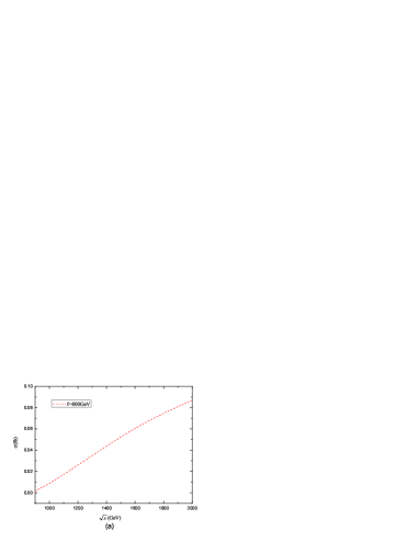
Figure 2: The production cross section $\sigma$ as functions of the center-of-mass energy $\sqrt{s}$ (a) and the scale $f$(b).

In Fig.2(a), we discuss the dependance of the production cross section $\sigma$ on the center-of-mass energy $\sqrt{s}$ for $f=800$GeV. We can see that the cross section $\sigma$ becomes lager with the $\sqrt{s}$ increasing.

In Fig.2(b), we discuss the dependance of the production cross section $\sigma$ on the scale $f$ for $\sqrt{s}=1500\textmd{GeV},2000\textmd{GeV}$, respectively. We can see the $\sigma$ decreases as the scale $f$ increases, which means that the vector-like top quark production cross section decouples with the scale $f$ increasing. The maximum of the production cross section can reach 0.17fb for $\sqrt{s}=1500$GeV and 0.25fb for $\sqrt{s}=2000$GeV, respectively. If we take the integrated luminosity $\mathcal{L}_{int}\simeq 500fb^{-1}$, there will be 125 events produced each year with $\sqrt{s}$=$2$TeV.

In Fig.3, we display the normalized transverse momentum distribution, the normalized distribution for the missing energy and the normalized rapidity of bottom quark of the process $e^{-}\gamma\rightarrow\nu_{e}\bar{t}b$ in the SM and the process $e^{-}\gamma\rightarrow\nu_{e}\bar{T}b$ in the LRTH model.

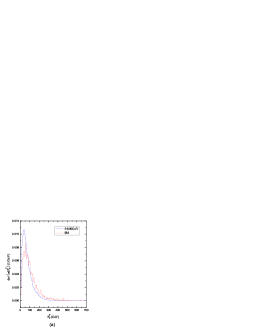
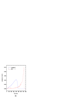
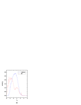
Figure 3: Normalized differential distributions for the SM top quark and the heavy top quark transverse momentum (a), the missing energy (b) and the rapidity of the bottom quark (c) for $\sqrt{s}=1500$GeV.

In Fig.3(a), we show the normalized transverse momentum distribution behaviour of the SM top quark and the heavy top quark. As the neutrino comes from the initial state positron after emitting a $W$ boson, the heavy top quark transverse momentum peaks at $\sim M_{W}/2$, which is very similar to the transverse momentum distribution behaviour of the SM top quark.

In Fig.3(b), we show the normalized distribution for the missing energy $\not\!\!\!E_{T}$ carried by the final-state neutrino. Compared with the SM top quark, the peak of the normalized distribution moves to the low energy region. With the scale $f$ increasing, this peak of the normalized distribution moves to the left. If we take a relevant missing energy $\not\!\!\!E_{T}$ cut, such as $\not\!\!\!E_{T}<500$GeV for $f=800$GeV, the SM background can be suppressed effectively. Considering the subsequent decay of the heavy top quark, the main signal is 4 b jets + one charged lepton (e or $\mu$) + energy $\not\!\!\!E_{T}$. Because the additional b jet carries off energy, the peak of the missing energy $\not\!\!\!E_{T}$ in the LRTH model is lower than the peak in the SM.

In Fig.3(c), we show the normalized rapidity distribution of bottom quark. The $WW\gamma$ diagram (Fig.1(a))corresponds to a virtual $W$ boson moving in the positive rapidity region to balance the $\nu$ emitted from the incoming $e^{-}$. This virtual $W$ boson’s decay products, the $b$ and $\bar{t}$ quarks, lead to the small kink in the right region. By contrast, the same thing happens in the process $e^{-}\gamma\rightarrow\nu_{e}\bar{T}b$, but the difference is that the kink is smaller due to the large mass of the heavy top quark.

IV Conclusions

In this paper, we studied the single vector-like top production process $e^{-}\gamma\rightarrow\nu_{e}\bar{T}b$ in the LRTH model. The result shows that there will be 125 events produced each year with $\sqrt{s}$=$2$TeV and the integrated luminosity $\mathcal{L}_{int}\simeq 500fb^{-1}$ at small value of the scale $f$ around 650 GeV. Now, by the b-quark tagging efficiency of $70\%$b-tagging and the relevant missing energy $\not\!\!\!E_{T}$ cut, this new effects will help to test the LRTH model and probe the new physics at the ILC.

References

• (1) F. Abe et al. (CDF Collaboration). Phys. Rev. Lett., 1995,74: 2626; S. Abachi et al. (D0 Collaboration). Phys. Rev. Lett., 1995,74: 2632.
• (2) Z. Chacko, H. S. Goh, R. Harnik. Phys. Rev. Lett., 2006,96: 231802; Z. Chacko, Y. Nomura, M. Papucci et al. JHEP, 2006,0601: 126; Z. Chacko, H. S. Goh, R. Harnik. JHEP, 2006,0601: 108; A. falkowski, S. Pokorski, M. Schmaltz. Phys. Rev. D, 2006,74: 035003.
• (3) Hock-Seng Goh, SU Shu-Fang. Phys. Rev. D, 2007,75: 075010; LIU Yao-Bei, WANG Xue-Lei. Int. J. Mod. Phys. A, 2010,25: 5885.
• (4) J. Brau, Y. Okada, N. Walker. arXiv:0712.1950; Abdelhak Djouadi, Joseph Lykken, Klaus MΓΆnig et al. arXiv:0709.1893; N. Phinney, N. Toge, N. Walker. arXiv: 0712.2361; T. Behnke, C. damerell, J. Jaros et al. arXiv:0712.2356; I. F. Ginzburg, G. L. Kothkin, V. G. Serbo et al. Nucl. Instr. Meth., 1983,205: 47.
• (5) CAO Qing-Hong, Jose Wudka. Phys. Rev. D, 2006,74: 094015; Jae Yong Lee. JHEP, 2004,0412: 065; E. Boos, M. Dubinin, A. Pukhov et al. Eur. Phys. J. C, 2001,21: 81-91; LIU Yao-Bei, WANG Xue-Lei, CAO Yong-Hua. Chin. Phys. Lett., 2007,24: 57-60; LIU Yao-Bei, SHEN Jie-Fen, WANG Xue-Lei. arXiv:hep-ph/0610350; SHEN Jie-Fen, CUI Xiao-Min, LI Yu-Qi et al. Chin. Phys. Lett., 2011,28(11): 111203; YUE Chong-Xing, YANG Hui-Di, MA Wei. Nucl. Phys. B, 2009,818: 1-16.
• (6) Z. Chacko, H. S. Goh, R. Harnik. JHEP, 2006,0601: 108.
• (7) Hock-Seng Goh, SU Shu-Fang. Phys. Rev. D, 2007,75: 075010.
• (8) G. Jikia. Nucl. Phys. B, 1992,374: 83; O. J. P. Eboli et al. Phys. Rev.D, 1993,47: 1889.
• (9) K. Nakamura et al. (Particle Data Group). J. Phys. G, 2010,37: 075021.
• (10) ATLAS Collaboration. arXiv:1210.5468.
• (11) CMS Collaboration. arXiv:1203.5410.
• (12) S. Godfrey, P. Kalyniak, A. Tomkins. arXiv:hep-ph/0511335; S. Hillert on behalf of the LCFI collaboration. LCWS-2005-0313, Mar 2005; A. Belyaev, T. Lastovicka, A. Nomerotski et al. Phys. Rev. D, 2010,81: 035011.