Trace distance and linear entropy of qubit states: Role of initial qubit-environment correlations

Abstract

The role of initial qubit–environment correlations on trace distance between two qubit states is studied in the framework of non–Markovian pure dephasing. The growth of mixedness of reduced state quantified by linear entropy is shown to be related to the degree of initial qubit–environment correlations.

Keywords: system–environment correlations, reduced dynamics, trace distance, dephasing

1. Introduction

In quantum mechanics, a state of a system is defined by a density matrix $\rho$. Nowadays, the state can be completely determined by the procedure which is called quantum tomography. Due to the fundamental limitations related to the Heisenberg uncertainty principle and the no-cloning theorem [1], one cannot perform an arbitrary sequence of measurements on a single system without inducing on it a back-action of some sort. On the other hand, the no-cloning theorem forbids to create a perfect copy of the system without already knowing its state in advance. Thus, there is no way out, not even in principle, to infer the quantum state of a single system without having some prior knowledge on it [2]. However, it is possible to reconstruct the unknown quantum state of a system when an ensemble of identical copies are available in the same state, so that a series of ideal measurements can be performed on each copy, for more information see e.g. [3, 4].

Manipulation on quantum states in atomic, molecular and optical systems is an important problem in contemporary physics research, with many types of experiments aimed at applications ranging from metrology to quantum computation, quantum cryptography and quantum-state engineering. It naturally arises the question on the relation between states before and after the manipulation and the extend to which states are similar or different. For example, are the output states more distinguishable or less distinguishable than the input states; do they behave in a similar way or not. The answer in not simple because it depends on a distinguishability measure. In literature one can find many examples of distinguishability measures which a part are based on the notion of a distance $D[\rho_{1},\rho_{2}]$ between two states $\rho_{1}$ and $\rho_{2}$. The distance can be quantified by a metric which has the following properties:
(i) non-negativity $D[\rho_{1},\rho_{1}]\geq 0$,
(ii) identity of indiscernibles $D[\rho_{1},\rho_{2}]=0$ if and only if $\rho_{1}=\rho_{2}$,
(iii) symmetry $D[\rho_{1},\rho_{2}]=D[\rho_{2},\rho_{1}]$,
(iv) the triangle inequality $D[\rho_{1},\rho_{2}]\leq D[\rho_{1},\rho_{3}]+D[\rho_{3},\rho_{2}]$.

In fact, the first condition is implied by the others. Because there are infinitely many metrics, the problem arises which metric is proper [5]. The most popular distance measures include the trace distance, Hilbert-Schmidt distance, Bures distance, Hellinger distance and Jensen-Shannon divergence [5, 6, 7, 8, 9, 10].

Majority of description of a general state-transformation is given in terms of the so-called quantum operation (also named as quantum dynamical map, quantum process or quantum channel) ${\cal E}$, i.e. by a linear, trace-preserving (more generally: trace non-increasing) completely positive map. Let us recall that the quantum operation $\cal E$ defined on the whole space of operators $\rho$ on the Hilbert space is contractive with respect to a given distance $D[\rho_{1},\rho_{2}]$ if

$$D[{\cal E}(\rho_{1}),{\cal E}(\rho_{2})]\leq D[\rho_{1},\rho_{2}].$$ (1)

It implies that two quantum states do not become more distinguishable under the action of quantum operation.

Real quantum systems are typically open, i.e. they interact with environment. Dynamics of such systems is not unitary and in general it is even not described by quantum operation. To understand it, let us assume that the total system $S$ + environment $E$ is closed and its unitary dynamics is determined by the total Hamiltonian

$$H=H_{S}\otimes{\mathbb{I}}_{E}+H_{I}+{\mathbb{I}}_{S}\otimes H_{E},$$ (2)

where $H_{S}$ is the Hamiltonian of the system $S$, $H_{E}$ is the Hamiltonian of the environment $E$ and $H_{I}$ describes the system-environment interaction. The operators ${\mathbb{I}}_{S}$ and ${\mathbb{I}}_{E}$ are identity operators (matrices) in corresponding Hilbert spaces of the system $S$ and the environment $E$, respectively. Let the initial state $\varrho$ of total system $S+E$ is determined by the density operator

$$\varrho=\varrho^{SE}(0).$$ (3)

Then the state of the system $S$ at time $t>0$ is determined by the reduced dynamics,

$$\rho(t)=\mbox{Tr}_{E}\{\varrho^{SE}(t)\}=\mbox{Tr}_{E}\{U(t)\ \varrho^{SE}(0)\ U^{\dagger}(t)\},\quad U(t)=\exp[-iHt/\hbar].$$ (4)

Because the partial trace $\mbox{Tr}_{E}$ is a quantum operation, it defines the trace preserving positive map $S+E\to S$:

$$\varrho^{SE}(0)\to\Lambda_{t}\varrho^{SE}(0)=\mbox{Tr}_{E}\{U(t)\ \varrho^{SE}(0)\ U^{\dagger}(t)\}.$$ (5)

In the case when the initial state is a non-correlated state, i.e. when it is a product state

$$\varrho^{SE}(0)=\rho_{S}\otimes\omega^{E},$$ (6)

where $\rho_{S}$ is an arbitrary initial state of the system $S$ and $\omega^{E}$ is a fixed initial state of the environment $E$, the relation

$$\rho_{S}\to\Phi_{t}\rho_{S}=\mbox{Tr}_{E}\{U(t)\ \rho_{S}\otimes\omega^{E}\ U^{\dagger}(t)\}$$ (7)

defines a trace preserving quantum operation $S\to S$ (into itself) which is also called a completely positive quantum dynamical map. Let ${\cal E}={\Phi_{t}}$ is such that $\rho^{\Phi}(t)={\Phi_{t}}\rho(0)$, where $\rho(0)$ is an initial state of the system $S$. Then contractivity (1) means that

$$D[\rho^{\Phi}_{1}(t),\rho^{\Phi}_{2}(t)]\leq D[\rho_{1}(0),\rho_{2}(0)]$$ (8)

for any two initial states $\rho_{1}(0)$ and $\rho_{2}(0)$ of the system $S$. As a consequence, the distance between two system states cannot increase in time and the distinguishability of any states can not increase above its initial value.

Now, let the initial state $\varrho^{SE}(0)$ is not a product state. It means that the system $S$ is initially correlated with its environment $E$. Let ${\cal E}={\Lambda_{t}}$ is such that $\rho^{\Lambda}(t)={\Lambda_{t}}\varrho^{SE}(0)$, where $\varrho^{SE}(0)$ is an initial state of the total system $S$. Then contractivity (1) means that

$$D[\rho^{\Lambda}_{1}(t),\rho^{\Lambda}_{2}(t)]\leq D[\rho_{1}^{SE}(0),\rho_{2}^{SE}(0)].$$ (9)

Note that in the left hand side of this relation there are two states $\rho^{\Lambda}_{1}(t)$ and $\rho^{\Lambda}_{2}(t)$ the system $S$ while in the right hand side there are two states $\rho_{1}^{SE}(0)$ and $\rho_{2}^{SE}(0)$ of the total system $S+E$. In this case, one cannot say whether the distance between two states of the system $S$ decreases or not because the relation (9) does not imply the inequality

$$D[\rho^{\Lambda}_{1}(t),\rho^{\Lambda}_{2}(t)]\leq D[\rho_{1}(0),\rho_{2}(0)],$$ (10)

where

$$\rho_{i}(0)=\mbox{Tr}_{E}\{\varrho^{SE}_{i}(0)\}\quad i=1,2$$ (11)

is the initial reduced state of the system $S$.

The formal relation

$$\rho_{S}=\mbox{Tr}_{B}\{\varrho^{SE}(0)\}\to W_{t}\rho_{S}=\mbox{Tr}_{E}\{U(t)\ \varrho^{SE}(0)\ U^{\dagger}(t)\}$$ (12)

is not generally a quantum operation. Moreover, $W_{t}$ is not even a map because many different $\varrho^{SE}(0)$ reduce to the same $\rho_{S}$ and for the same $\rho_{S}$ one can obtain several different $W_{t}\rho_{S}$. Therefore in general the inequality (10) need not be fulfilled in the case of initially correlated state of $S+E$.

As an example of the distance measure let us recall the trace distance defined by the relation

$$D_{T}[\rho_{1},\rho_{2}]=\frac{1}{2}\mbox{Tr}\sqrt{(\rho_{1}-\rho_{2})^{2}}$$ (13)

which is limited to the unit interval,

$$0\leq D_{T}[\rho_{1},\rho_{2}]\leq 1.$$

From the Ruskai theorem [11] follows that the quantum operation $\cal E$ is a contraction with respect to the trace distance. In such a case, the relations (8) and (9) are satisfied when distance $D=D_{T}$ is the trace distance. Therefore the trace distance between two states of the system $S$ cannot increase in time when the system $S$ is initially non-correlated with its environment and the distinguishability of any system states can not increase above an initial value. In the case when the system $S$ is correlated with the environment $E$, one cannot say whether the distance between two states of the system $S$ decreases or not because the relation (10) does not hold in a general case.

From the above it follows that the trace distance $D_{T}[\rho_{1}(t),\rho_{2}(t)]$ between two states $\rho_{1}(t)$ and $\rho_{2}(t)$ of the system $S$ can grow above its initial value $D_{T}[\rho_{1}(0),\rho_{2}(0)]$ only in two cases:
(A) when the system $S$ is initially correlated with the environment $E$ or
(B) when the system $S$ is initially non-correlated with the environment $E$ and in the relation (7) there are two different initial states $\omega^{E}_{1}$ and $\omega^{E}_{2}$ of the environment $E$, i.e. when

$$\rho_{1}(t)=\mbox{Tr}_{B}\{U(t)\ \rho\otimes\omega^{E}_{1}\ U^{\dagger}(t)\},$$

$$\rho_{2}(t)=\mbox{Tr}_{B}\{U(t)\ \rho\otimes\omega^{E}_{2}\ U^{\dagger}(t)\}.$$ (14)

We should remember that contractivity of reduced dynamics is not a universal feature but depends on chosen metric and therefore decrease or increase of distances between two states can depend on the metric [12]. Contractivity of quantum evolution can break down when the system $S$ is initially correlated with its environment [13, 14] and implications of such correlations have been studied in various context [14, 15]. Examples of an exact reduced dynamics which fail contractivity with respect to the trace distance are studied in Refs. [16, 17, 12]. Two experiments on initial system-environment correlations have recently been conducted in optical systems [18].

In the paper, we study the role of initial system-environment states on the trace distance of states and linear entropy for the reduced dynamics. In Sec. 2, we define a quantum open system. It is a two-level system (qubit) interacting with an infinite bosonic environment. We consider a pure dephasing interaction between the qubit and the environment [19] and we ignore the energy decay of the qubit. This assumption is reasonable since in some cases the phase coherence decays much faster than the energy. We derive the exact reduced dynamics of the qubit for a particular initial correlated qubit-environment state. Properties of time evolution of the distance between two states of the qubit are demonstrated in Sec. 3. In the same section we analyze the mixedness of reduced state quantified by entropic measure. Finally, Sec. 4 provides summary and some conclusions.

2. Qubit dephasingly coupled to infinite bosonic environment

In this section, we consider the same model as in our previous papers [16, 12]. For the readers convenience and to keep the paper self-contained, we repeat all necessary definitions and introduce notations. The model consists of a qubit $Q$ (two-level system) coupled to its environment $E$ and we limit our considerations to the case when the process of energy dissipation is negligible and only pure dephasing is acting as the mechanism responsible for decoherence of the qubit dynamics [19]. Such a decoherence mechanism can be described by the total Hamiltonian (with $\hbar=1$)

$$H=H_{Q}\otimes{\mathbb{I}}_{E}+{\mathbb{I}}_{Q}\otimes H_{E}+S^{z}\otimes H_{I},$$ (15)

$$H_{Q}=\varepsilon S^{z},\quad H_{E}=\int_{0}^{\infty}d\omega\,h(\omega)a^{\dagger}(\omega)a(\omega),$$ (16)

$$H_{I}=\int_{0}^{\infty}d\omega\left[g^{*}(\omega)a(\omega)+g(\omega)a^{\dagger}(\omega)\right],$$ (17)

where $S^{z}$ is the z-component of the spin operator and is represented by the diagonal matrix $S^{z}=diag[1,-1]$ of elements $1$ and $-1$. The parameter $\varepsilon$ is the qubit energy splitting, ${\mathbb{I}}_{Q}$ and ${\mathbb{I}}_{E}$ are identity operators (matrices) in corresponding Hilbert spaces of the qubit $Q$ and the environment $E$, respectively. The operators $a^{\dagger}(\omega)$ and $a(\omega)$ are the bosonic creation and annihilation operators, respectively. The real-valued spectrum function $h(\omega)$ characterizes the environment. The coupling is described by the function $g(\omega)$ and the function $g^{*}(\omega)$ is the complex conjugate to $g(\omega)$. The Hamiltonian (15) can be rewritten in the block–diagonal structure [20],

$$H=diag[H_{+},H_{-}],\quad H_{\pm}=H_{B}\pm H_{I}\pm\varepsilon{\mathbb{I}}_{B}.$$ (18)

As an example, we assume that at the initial time $t=0$ the composite wave function $|\Psi(0)\rangle$ of $S+E$ is given by the expression

$$|\Psi(0)\rangle=b_{+}|1\rangle\otimes|\Omega_{0}\rangle+b_{-}|-1\rangle\otimes|\Omega_{\lambda}\rangle.$$ (19)

The states $|1\rangle$ and $|-1\rangle$ denote the excited and ground state of the qubit, respectively. The non-zero complex numbers $b_{+}$ and $b_{-}$ are chosen in such a way that the condition $|b_{+}|^{2}+|b_{-}|^{2}=1$ is satisfied. The state $|\Omega_{0}\rangle$ is the ground (vacuum) state of the environment and

$$|\Omega_{\lambda}\rangle=C_{\lambda}^{-1}\,\left[(1-\lambda)|\Omega_{0}\rangle+\lambda|\Omega_{f}\rangle\right],$$ (20)

where $|\Omega_{f}\rangle=D(f)|\Omega_{0}\rangle$ is the coherent state. The displacement (Weyl) operator $D(f)$ reads [21]

$$D(f)=\exp\left\{\int_{0}^{\infty}d\omega\left[f(\omega)a^{\dagger}(\omega)-f^{*}(\omega)a(\omega)\right]\right\}$$ (21)

for an arbitrary square–integrable function $f$. The constant $C_{\lambda}$ normalizes the state (19) and is given by the expression

$$C_{\lambda}^{2}=(1-\lambda)^{2}+\lambda^{2}+2\lambda(1-\lambda)Re\langle\Omega_{0}|\Omega_{f}\rangle,$$ (22)

where ${Re}$ is a real part of the scalar product $\langle\Omega_{0}|\Omega_{f}\rangle$ of two states in the environment Hilbert space. The correlated initial state (19) is in the form similar to that in Ref. [16]. The parameter $\lambda\in[0,1]$ controls the strength of initial correlations of the qubit with environment. For $\lambda=0$ the qubit and the environment are initially uncorrelated while for $\lambda=1$ the correlation is most prominent for the assumed class of initial states.

The initial wave function (19) of the isolated system $S+E$ evolves unitarily according to the Hamiltonian (15) and reads

$$|\Psi(t)\rangle=b_{+}|1\rangle\otimes|\psi_{+}(t)\rangle+b_{-}|-1\rangle\otimes|\psi_{-}(t)\rangle,$$ (23)

where

$$|\psi_{+}(t)\rangle = \exp(-iH_{+}t)|\Omega_{0}\rangle,$$

$$|\psi_{-}(t)\rangle = \exp(-iH_{-}t)|\Omega_{\lambda}\rangle.$$ (24)

The state of the total system is a pure state and the corresponding density matrix $\varrho(t)=|\Psi(t)\rangle\langle\Psi(t)|$. In turn, the partial trace $\mbox{Tr}_{E}$ over the environment degrees of freedom yields the density matrix $\rho_{\lambda}(t)=\mbox{Tr}_{E}\varrho(t)$ of the qubit. In the base $\{|1\rangle,|-1\rangle\}$, it takes the matrix form

$$\rho_{\lambda}(t)=\left(\begin{array}[]{cc}|b_{+}|^{2}&b_{+}b_{-}^{*}\,A_{\lambda}(t)\\ b_{+}^{*}b_{-}\,A_{\lambda}^{*}(t)&|b_{-}|^{2}\end{array}\right),$$ (27)

where the decoherence factor $A_{\lambda}(t)$ is given by

$$A_{\lambda}(t)=C_{\lambda}^{-1}\,e^{-2i\varepsilon t-r(t)}\left[1-\lambda+\lambda e^{-2i\Phi(t)+s(t)}\right],$$ (28)

and [20]

$$r(t) = 4\int_{0}^{\infty}d\omega g_{h}^{2}(\omega)\left[1-\cos(\omega t)\right],\quad\quad\quad\quad\quad$$ (29)

$$s(t) = 2\int_{0}^{\infty}d\omega g_{h}(\omega)f(\omega)\left[1-\cos(\omega t)\right]\quad$$ (30)

$$- \frac{1}{2}\int_{0}^{\infty}d\omega f^{2}(\omega),$$

where $g_{h}(\omega)=g(\omega)/\omega$ and

$$\Phi(t)=\int_{0}^{\infty}d\omega g_{h}(\omega)f(\omega)\sin(\omega t).$$ (31)

Without loss of generality we have assumed in Eqs. (29)-(31) that the functions $g(\omega)$ and $f(\omega)$ are real valued and the energy spectrum function $h(\omega)=\omega$.

Now, let us consider the second class of initial states of the total system. We assume that the system-environment initial state is mixed and given by the product state:

$$\varrho_{p}(0)=\rho_{\lambda}(0)\otimes|\Omega_{0}\rangle\langle\Omega_{0}|,$$ (32)

where

$$\rho_{\lambda}(0)=\mbox{Tr}_{E}|\Psi(0)\rangle\langle\Psi(0)|$$ (33)

is the marginal qubit state and $|\Psi(0)\rangle$ is defined by Eq. (19). From the relation

$$\rho_{p}(t)=\mbox{Tr}_{E}\{\mbox{e}^{-iHt}\ \rho_{\lambda}(0)\otimes|\Omega_{0}\rangle\langle\Omega_{0}|\ \mbox{e}^{-iHt}\}$$ (34)

we obtain the reduced dynamics of the qubit in the case of the initial uncorrelated qubit-environment state. It can be expressed in the matrix form as:

$$\rho_{p}(t)=\left(\begin{array}[]{cc}|b_{+}|^{2}&b_{+}b_{-}^{*}\,A_{\lambda}(0)A_{0}(t)\\ b_{+}^{*}b_{-}\,A^{*}_{\lambda}(0)A^{*}_{0}(t)&|b_{-}|^{2}\end{array}\right).$$ (37)

Properties of the trace distance between qubit states subjected to reduced dynamics (27) and (37) are presented in the next section. We stress that that initial states (19) and (32) of the total systems are different because the initial environmental states are different. However, the reduced initial states of the qubit are the same in both cases.

3. Properties of trace distance and linear entropy

Our model is still incomplete. We have to consider some models for the spectral density $g_{h}^{2}(\omega)$ of the environment, see Eqs.(29)-(31). We assume that for low frequencies it exhibits power–like frequency dependence and the frequency scale characterizes the cut-off frequency. An example of such a function is taken in the form [22]

$$g_{h}^{2}(\omega)=\alpha\,\omega^{\mu-1}\exp(-\omega/\omega_{c}),$$ (38)

where $\alpha>0$ is the qubit-environment coupling constant, $\omega_{c}$ is a cut-off frequency and $\mu>-1$ is the ”ohmicity” parameter: the case $-1<\mu<0$ corresponds to the sub–ohmic, $\mu=0$ to the ohmic and $\mu>0$ to super–ohmic environments, respectively. As it follows from our previous study [16], only in the case of super–ohmic environment, the trace distance can increase. Therefore below we analyze only this regime.

The second function we have to specify is the function $f(\omega)$ in Eq. (21) which determines the coherent state of the boson environment. We can choose any integrable function but for convenience we take the function

$$f^{2}(\omega) = \gamma\,\omega^{\nu-1}\exp(-\omega/\omega_{c}).$$ (39)

There is no deeper physical justification for it and the only reason for our choice is possibility to calculate explicit formulas for the functions in Eqs. (29)-(31). As a result one gets

$$r(t)=4\mathcal{L}(\alpha,\mu,t),\quad\quad\quad$$ (40)

$$s(t)=2\mathcal{L}(\sqrt{\alpha\gamma},(\mu+\nu)/2,t)-\frac{1}{2}\gamma\Gamma(\nu)\omega_{c}^{\nu},$$ (41)

$$\mathcal{L}(\alpha,\mu,t)=\alpha\Gamma(\mu)\omega_{c}^{\mu}\left\{1-\frac{\cos\left[\mu\arctan(\omega_{c}t)\right]}{(1+\omega_{c}^{2}t^{2})^{\mu/2}}\right\},$$ (42)

$$\Phi(t)=\sqrt{\alpha\gamma}\;\Gamma\left(\kappa\right)\omega_{c}^{\kappa}\;\frac{\sin\left[\frac{\mu+\nu}{2}\arctan(\omega_{c}t)\right]}{(1+\omega_{c}^{2}t^{2})^{\kappa/2}},$$ (43)

where $\kappa=(\mu+\nu)/2$ and $\Gamma(z)$ is the Euler gamma function.

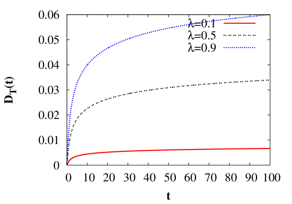
Fig. 1: (Color online) Time evolution of the trace distance $D_{T}(t)\equiv D_{T}[\rho_{\lambda}(t),\rho_{p}(t)]$ between two qubit states (27) and (37) for selected values of the correlation parameter $\lambda$. Time is in unit of $\omega_{c}$, the dimensionless coupling $\alpha\omega_{c}^{\mu}=0.01$ and $\gamma\omega_{c}^{\nu}=0.05$. The remaining parameters are: $\varepsilon=1,\mu=0.01$, $\nu=0.2$ and $|b_{+}^{(1)}|^{2}=|b_{+}^{(2)}|^{2}=1/2$.

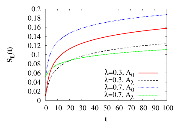
Fig. 2: (Color online) Time evolution of the linear entropy of two qubit states (27) indicated by $A_{\lambda}$ and (37) indicated by $A_{0}$ for selected values of the correlation parameter $\lambda$. Time is in unit of $\omega_{c}$, the dimensionless coupling $\alpha\omega_{c}^{\mu}=0.01$ and $\gamma\omega_{c}^{\nu}=0.05$. The remaining parameters are: $\varepsilon=1,\mu=0.01$, $\nu=0.2$ and $|b_{+}^{(1)}|^{2}=|b_{+}^{(2)}|^{2}=1/2$.

We analyze the distance between two qubit states for the case when two corresponding initial states of the total system are given by Eqs. (19) and (32), respectively. It is the case when at initial time $t=0$ the first state of the qubit is correlated with its environment and the second state is non-correlated. In Fig. 1 we present time evolution of the trace distance $D_{T}(t)=D[\rho_{\lambda}(t),\rho_{p}(t)]$ between two qubit states (27) and (37) for selected values of the correlation parameter $\lambda$. The first observation is the monotonic increase of the distance as time grows and the distance saturates in the long-time limit. The second observation is that increase of the correlation parameter $\lambda$ enhances distinguishability of two states and the distance between two qubit states grows.

Quantum dynamics of an open system results in growing (or at least non–lowering) ’mixedness’ of the reduced state. Equivalently, one may discuss the problem of the entropy production resulting from the dephasing process. Here, as a simplest measure of the information loss due to system-environment interaction we adapt the linear entropy

$$S_{L}[\rho]=1-\mbox{Tr}(\rho^{2})$$ (44)

of any reduced states $\rho$. It takes the form

$$S_{L}[\rho_{\lambda}]=1-\left[|b_{+}|^{4}+|b_{-}|^{4}+2|b_{+}|^{2}|b_{-}|^{2}|A_{\lambda}(t)|^{2}\right]$$ (45)

for the state (27) and

$$S_{L}[\rho_{p}]=1-\left[|b_{+}|^{4}+|b_{-}|^{4}+2|b_{+}|^{2}|b_{-}|^{2}|A_{\lambda}(0)A_{0}(t)|^{2}\right]$$ (46)

for the state (37).

The linear entropy can range between zero, corresponding to a completely pure state, and $1/2$ corresponding to a completely mixed state. In Fig. 2, we compare time evolution of the linear entropy for both types of models Eqs. (27,37). It is seen that the difference $S_{L}[\rho_{p}]-S_{L}[\rho_{\lambda}]$ is greater when $\lambda$ is greater. It means that for any time $t>0$ the mixedness of the reduced state is smaller when the qubit is initially correlated with its environment in comparison to the case when the initial state is uncorrelated. Moreover, if the degree of correlation grows the mixedness decreases. The results exemplified in Fig. 2 allow to conclude that

$$S_{L}[\rho_{p}]\geq S_{L}[\rho_{\lambda}].$$ (47)

As the expression for both $S_{L}[\rho_{\lambda}]$ and $S_{L}[\rho_{p}]$ are known, it can be proven using straightforward analytic methods. Indeed, from (45) and (46), it follows that (47) holds true if $|A_{\lambda}(t)|^{2}\geq|A_{\lambda}(0)A_{0}(t)|^{2}$. In turn, it is equivalent to the requirement $s(t)\geq s(0)$ which is true as follows from Eq. (30).

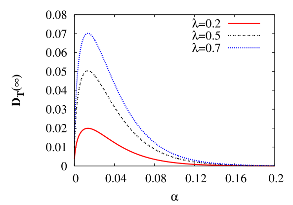
Fig. 3: (Color online) Long–time characteristics of the trace distance between two qubit states (27) and (37) as a function of the qubit-environment coupling constant $\alpha$ in (38) for selected values of the correlation parameter $\lambda$. Time is in unit of $\omega_{c}$, $\gamma\omega_{c}^{\nu}=0.05$. The remaining parameters are: $\varepsilon=1,\mu=0.01$, $\nu=0.2$ and $|b_{+}^{(1)}|^{2}=|b_{+}^{(2)}|^{2}=1/2$.

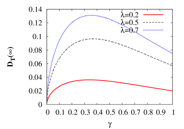
Fig. 4: (Color online) Long–time characteristics of the trace distance between two qubit states Eqs. (27) and (37) as a function of the amplitude $\gamma$ Eq,(39) for selected values of the correlation parameter $\lambda$. Time is in unit of $\omega_{c}$, the dimensionless coupling $\alpha\omega_{c}^{\mu}=0.01$. The remaining parameters are: $\varepsilon=1,\mu=0.01$, $\nu=0.2$ and $|b_{+}^{(1)}|^{2}=|b_{+}^{(2)}|^{2}=1/2$.

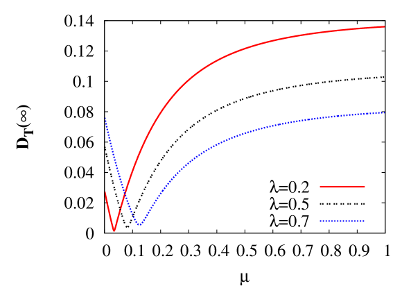
Fig. 5: (Color online) Long–time characteristics of the trace distance between two qubit states (27) and (37) as a function of the ’ohmicity parameter’ $\mu$ in Eq.(38) for selected values of $\lambda$. Time is in unit of $\omega_{c}$, the dimensionless coupling is kept fixed: $\alpha\omega_{c}^{\mu}=0.01$ and $\gamma\omega_{c}^{\nu}=0.05$. The remaining parameters are: $\varepsilon=1$, $\nu=0.2$ and $|b_{+}^{(1)}|^{2}=|b_{+}^{(2)}|^{2}=1/2$.

Now, we analyze the long time limit of the trace distance between two qubit states, $D_{T}(\infty)=\lim_{t\to\infty}D_{T}[\rho_{\lambda}(t),\rho_{p}(t)]$. The dependence of $D_{T}$ on the qubit-environment coupling constant $\alpha$, which occurs in the spectral density (38), exhibits a bell-shaped extremum and then the optimal coupling exists which maximizes the trace distance, see Fig. 3. The maximum is the most pronounced for a strong initial correlations. For weak and strong coupling, the distance tends to zero. In Fig. 4, we depict the influence of the parameter $\gamma$ which characterizes the coherent state of environment. One can also observe a maximum of the distance. Finally, in Fig. 5, we investigate how the spectral properties of the environment, encoded in the ’ohmicity’ parameter $\mu$, influences on the distance. The most important observation is the occurrence of minimum in distance for a particular value of $\mu$. The strong superomic environment is more desired for distingushability of qubit states.

4. Summary

According to Ref. [17], an increase of the distance can be interpreted in terms of the exchange of information between the system and its environment. If the distance increases over its initial value, information which is locally inaccessible at the initial time is transferred to the open system. This transfer of information enlarges the distinguishability of the open-system states which suggests various ways for the experimental detection of initial correlations. The trace metric is one of the most important measures of a distance between states in quantum information processing. Moreover, it has a physical interpretation as a measure of state distinguishability.

With this work, we have studied the role of initial qubit-environment correlations and analyzed two characteristics: trace distance between two qubit states and the linear entropy. We have demonstrated that the trace distance exhibits a rich diversity of characteristics and is sensitive to selected parameters like coupling strength of the qubit and environment. In particular, depending on the chosen parameter regime, we can identify optimal regimes where the distance is locally maximal and distinguishability of the qubit states can be maximal. Moreover, the trace distance increases as time grows and saturates in the long-time limit. The increase of the correlation parameter $\lambda$ enhances distinguishability of two states and the distance between two qubit states grows. The results on the trace distance presented here extend findings of Refs. [16] and [12], where the initial state of the composite system was always a pure state and the initial state of the environment was a mixed state. Here we include the case of a mixed state of the composite system and a pure environment state. Here and there, the initial state of the qubit is mixed.

We have also considered a linear entropy of the reduced state which monotonically grows as time grows (the reduced state is more and more mixed). The impact of initial correlations on the linear entropy is also crucial: For any time $t>0$ the mixedness of the reduced state (i.e. how much the initial state is far from being pure) is smaller when the qubit is initially correlated with its environment and if the degree of correlation grows the mixedness decreases. This work could be continued to extend future theoretical studies. In particular, it would be interesting to study other classes of initial correlations and their impact on distance properties of qubit states and other characteristics of the quantum open systems.

References

- [1] W. K. Wootters and W. H. Zurek, Nature 299, 802 (1982); H. P. Yuen, Phys. Lett. A 113, 405 (1986).
- [2] G. M. D’Ariano and H. P. Yuen, Phys. Rev. Lett. 76, 2832 (1996).
- [3] G. Mauro D’Ariano, Matteo G. A. Paris, Massimiliano F. Sacchi, Advances in Imaging and Electron Physics Vol. 128, p. 205-308 (2003)
- [4] J. B. Altepeter, E. R. Jeffrey, and P. G. Kwiat, “Photonic State Tomography”, Advances in AMO Physics, Vol. 52 (Elsevier, 2006); M. Cramer, M. B. Plenio, S. T. Flammia, R. Somma, D. Gross, S. D. Bartlett, O. Landon-Cardinal, D. Poulin, and Yi-Kai Liu, ”Efficient quantum state tomography”, Nat. Commun. 1:149 doi: 10.1038/ncomms1147 (2010).
- [5] A. Gilchrist, N. K. Langford, and M. A. Nielsen, Phys. Rev. A 71, 062310 (2005).
- [6] S. Luo and Q. Zhang, Phys. Rev. A 69, 032106 (2004).
- [7] A. P. Majtey, P. W. Lamberti, and D. P. Prato, Phys. Rev. A 72, 052310 (2005).
- [8] V. V. Dodonov, O. V. Man’ko, V. I. Man’ko, and A. Wunsche, J. Modern Optics 47, 633 (2000).
- [9] M. A. Nielsen and L. I. Chuang, Quantum Computation and Quantum Information (Cambridge University Press, Cambridge, U.K., 2000).
- [10] I. Bengtsson and K. Życzkowski, Geometry of quantum states: An Introduction to Quantum Entanglement (Cambridge University Press, Cambridge, 2006).
- [11] M. B. Ruskai, Rev. Math. Phys. 6, 1147 (1994).
- [12] J. Dajka, Łuczka and P. Hänggi, Phys. Rev. A 84, 032120 (2011).
- [13] P. Pechukas, Phys. Rev. Lett. 73, 1060 (1994); P. Pechukas, Phys. Rev. Lett. 75, 3021 (1995). P. Stelmachovic and V. Buzek, Phys. Rev. A 64, 062106 (2001); N. Boulant, J. Emerson, T.F. Havel, D.G. Cory, and S. Furuta, J. Chem. Phys. 121, 2955 (2004); T. F. Jordan, A. Shaji, E. C. G. Sudarshan, Phys. Rev. A 70, 052110 (2004).
- [14] K. M. F. Romero, P. Talkner, and P. Hänggi, Phys. Rev. A 69, 052109 (2004).
- [15] A. Smirne, H.-P. Breuer, J. Piilo, and B. Vacchini, Phys. Rev. A 82, 062114 (2010); Hua-Tang Tan and Wei-Min Zhang, Phys. Rev. A 83, 032102 (2010); M. Ban, S. Kitajima, and F. Shibata, Phys. Lett. A375, 2283 (2011); Phys. Rev. A 84, 042115 (2011).
- [16] J. Dajka and J. Łuczka, Phys. Rev. A 82, 012341 (2010).
- [17] E.–M. Laine, J. Pilio and H.-P. Breuer, EPL 92, 60010 (2010).
- [18] Chuan-Feng Li, Jian-Shun Tang, Yu-Long Li, and Guang-Can Guo, Phys. Rev. A 83, 064102 (2011);A. Smirne, D. Brivio, S. Cialdi, B. Vacchini, and M. G. A. Paris, Phys. Rev. A 84, 032112 (2011).
- [19] J. Łuczka, Physica A 167, 919 (1990).
- [20] J. Dajka and J. Łuczka, Phys. Rev. A 77, 062303 (2008); J. Dajka, M. Mierzejewski, and J. Łuczka, Phys. Rev. A 79, 012104 (2009).
- [21] O. Brattelli and D. W. Robinson, Operator Algebras and Quantum Statistical Mechanics 2 (Springer, Berlin, 1997).
- [22] A. J. Legget, S. Chakravarty, A. T. Dorsey, Matthew P. A. Fisher, Anupam Garg, and W. Zwerger, Rev. Mod. Phys. 59, 1 (1987).