Fluctuations and correlations of a driven tracer in a hard-core lattice gas

Abstract

We consider a driven tracer particle (TP) in a bath of hard-core particles undergoing continuous exchanges with a reservoir. We develop an analytical framework which allows us to go beyond the standard force-velocity relation used for this minimal model of active microrheology and quantitatively analyze, for any density of the bath particles, the fluctuations of the TP position and their correlations with the occupation number of the bath particles. We obtain an exact Einstein-type relation which links these fluctuations in the absence of a driving force and the bath particles density profiles in the linear driving regime. For the one-dimensional case we also provide an approximate but very accurate explicit expression for the variance of the TP position and show that it can be a non-monotoneous function of the bath particles density: counter-intuitively, an increase of the density may increase the dispersion of the TP position. We show that this non trivial behavior, which could in principle be observed in active microrheology experiments, is induced by subtle cross-correlations quantified by our approach.

I Introduction

Active probe-based microrheology, which monitors the position of a tracer particle (TP) driven by an external force, has become a powerful experimental tool for the analysis of different systems in physics, chemistry and biology (see, e.g., Ref. Wilson and Poon (2011)). In the constant-forcing microrheology setup, a microscopic particle embedded in a sample is actively manipulated by applying a known force. One measures then the response of the TP and potentially the microstructural deformations of the medium to learn about its microrheological properties. From the theoretical point of view, an unresolved issue, which is disregarded in the available continuous analytical approaches, is to take into account explicitly the discreteness or ”granularity” of the medium Wilson and Poon (2011). This aspect becomes crucial when the probe and the medium particles have comparable sizes, e.g. in colloidal suspensions. In this regime, both fluctuations of the probe that can not be described correctly if the medium is treated as a continuous bath and super-diffusion regimes have been reported Wilson et al. (2011); Winter et al. (2012); Schroer and Heuer (2012); Bénichou et al. (2012); Harrer et al. (2012)

Within a broader context, modeling the response of a medium to a perturbation created by a tracer particle, biased by an external force, is a ubiquitous problem in physics, which has been the subject of a large number of theoretical works Marini Bettolo Marconi et al. (2008); Cugliandolo (2011); Gradenigo et al. (2012). The resulting stochastic dynamics of the whole system is however a many-body problem which is difficult (or even impossible) to solve even in the simplest case when the particle-particle interactions are a mere hard-core. For that reason, in most approaches the microscopic structure of the bath is not taken into account explicitly, and the response functions are determined instead by using some effective bath dynamics, modelled via Langevin or generalized Langevin Lizana et al. (2010) equations (see also Refs. Marini Bettolo Marconi et al. (2008); Cugliandolo (2011); Gradenigo et al. (2012)). While these approaches are rather efficient, they cannot account for the detailed correlations between the tracer particle and the fluctuating density profiles of the bath particles. In this paper, we show that these cross correlations are of crucial importance and can lead to non trivial effects beyond the usual analysis of the force-velocity relation. We predict in particular a non monotonic behavior of the variance of the tracer position with the density of the bath, that in principle could be observed in active microrheology experiments.

Our analysis relies on a model of driven tracer diffusion in a hard-core lattice gas, which appears as a minimal model of active microrheology that explicitly takes into account the dynamics of a bath of discrete particles: A TP driven by an external force performs a biased lattice random walk in a bath of hard-core particles, which themselves perform symmetric random walks constrained by the condition of a single occupancy of each lattice site.

At the theoretical level, the one dimensional version of this model is related to several well known models of out of equilibrium statistical physics. For example, in the absence of external driving, it reduces to the single file diffusion problem Harris (1965). In the absence of external driving and when additional adsorption/desorption processes with a reservoir of particles are considered, it corresponds to the so-called dynamical percolation Druger et al. (1983); Bénichou et al. (2000a). Last, in the case of a constant external forcing experienced by all the particles, it identifies with the asymmetric exclusion process, which has now become a paradigmatic model, both in the absence (see Chou et al. (2011) for a recent review) or in the presence Parmeggiani et al. (2003) of adsorption/desorption processes. This model of driven tracer diffusion has been investigated both in the physical Burlatsky et al. (1992, 1996); Bénichou et al. (1999); Bénichou et al. (2000b); Bénichou et al. (2001) and in the mathematical Landim et al. (1998); Komorowski and Olla (2005) literatures. Most of the obtained results, including proofs of the Einstein relation, are limited to the large time behavior of the mean position $\langle X_{tr}\rangle$ of the tracer particle and the stationary density profiles of the bath $\langle\eta_{\bf r}\rangle$, where $\eta_{\bf r}$ stands for the occupation number of the site ${\bf r}$ of the lattice, equal to 1 if occupied by a bath particle and 0 otherwise. A general method to analyze the fluctuations of the tracer position $\langle\delta X_{tr}^{2}\rangle$ and the cross-correlation functions of the form $\langle\delta X_{tr}\delta\eta_{\bf r}\rangle$ is still lacking .

Here, for this minimal model of active microrheology we develop a theoretical framework allowing to analytically determine these fluctuations in all regimes of bath particles density, and in principle for arbitrary dimension. More precisely, our main results obtained within this formalism are (i) An exact Einstein-type relation satisfied by the cross-correlations in the absence of a driving force and the density profiles of the bath particles in the linear-response regime. (ii) An explicit approximate but accurate expression for the variance of the tracer position in a one-dimensional case valid for any density. (iii) A finding that the variance of the position of the tracer can be a non-monotonic function of the density of bath particles, meaning that, counter-intuitively, an increase of the density of hard-core particles can increase the dispersion of the tracer position. We show that, in fact, subtle correlations between the tracer and the bath particles are responsible for this intriguing behavior. We anticipate that this striking effect could in principle be observed experimentally in the context of active microrheology.

II The model

Consider a $d$-dimensional hypercubic lattice of spacing $\sigma$ in contact with a reservoir of particles kept at a constant chemical potential (see figure 1). Suppose next that the particles in the reservoir may adsorb onto vacant lattice sites at a fixed rate $f/\tau^{*}$. The adsorbed particles may move randomly along the lattice by hopping at a rate $1/2d\tau^{*}$ to any of $2d$ neighboring lattice sites, which process is constrained by a hard-core exclusion preventing multiple occupancy of any of the sites. The adsorbed particles may desorb from the lattice back to the reservoir at rate $g/\tau^{*}$. The occupancy of lattice sites is described by the time-dependent Boolean variable $\eta_{{\bf r}}$, which assumes two values, $1$, if the site ${\bf r}$ is occupied by an adsorbed particle, and $0$, otherwise. Note that the mean density of the bath particles, $\langle\eta_{\bf r}\rangle$, approaches as $t\to\infty$ a constant value $\rho_{s}=f/(f+g)$ but the number of particles on the lattice is not explicitly conserved in such a dynamics.

At $t=0$ we introduce a TP, whose position at time $t$ is denoted as ${\bf R}_{tr}(t)$. The TP dynamics is different from that of the adsorbed particles in two aspects: first, it can not desorb from the lattice and second, it is subject to an external driving force E, which favors its jumps along the direction corresponding to the unit vector ${\bf e_{1}}$ of the lattice. Physically, such a situation is realized in the context of active microrheology where the force on the TP is classically exerted by magnetic tweezers Wilson and Poon (2011).

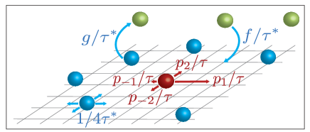
Figure 1: Model notations in the two-dimensional (2D) case.

The TP dynamics is defined in the usual fashion: We suppose that the tracer, which occupies the site ${\bf R}_{tr}$ at time $t$, waits an exponentially distributed time with mean $\tau$, and then attempts to hop onto one of $2d$ neighboring sites, ${\bf R}_{tr}+{\bf e}_{\bm{\nu}}$, where ${\bf e}_{\bm{\nu}}$ are $2d$ unit vectors of the hypercubic lattice. The jump direction is chosen according to the probability $p_{\nu}$, which obeys:

$$p_{\nu}=\exp\left[\frac{\beta}{2}({\bf E\cdot e}_{\nu})\right]\left/\sum_{\mu}\exp\left[\frac{\beta}{2}({\bf E\cdot e}_{\mu})\right]\right.,$$ (1)

where $\beta$ is the inverse temperature and $\sum_{\mu}$ denotes summation over all possible orientations of the vector ${\bf e}_{\mu}$. The hop is instantaneously fulfilled if the target site is vacant at this moment of time; otherwise, i.e., if the target site is occupied by any adsorbed particle, the jump is rejected and the tracer remains at its position.

III Evolution equations

We focus on the projection of the TP position $X_{tr}\equiv{\bf R}_{tr}\cdot{\bf e}_{1}$, which evolves in an infinitesimal time interval $\mathrm{d}t$ according to

$$X_{tr}(t+\mathrm{d}t)=\left\{\begin{array}[]{ll}X_{tr}(t)+\sigma,\mbox{ w.p. $\pi_{1}=p_{1}(1-\eta_{1})\mathrm{d}t$}\\ X_{tr}(t)-\sigma,\mbox{ w.p. $\pi_{-1}=p_{-1}(1-\eta_{-1})\mathrm{d}t$}\\ X_{tr}(t),\mbox{w.p. $1-\pi_{1}-\pi_{-1}$}\end{array}\right.$$

where w.p. stands for with probability. Averaging this equation, it is easy to find that the mean $\langle X_{tr}\rangle$ and the variance $\langle\delta X_{tr}^{2}\rangle$ of the TP position verify:

$$\frac{\mathrm{d}}{\mathrm{d}t}\langle X_{tr}(t)\rangle=\frac{\sigma}{\tau}\{p_{1}(1-k_{1})-p_{-1}(1-k_{-1})\},$$ (2)

and

$$\frac{\mathrm{d}}{\mathrm{d}t}\langle\delta X_{tr}(t)^{2}\rangle=\frac{\sigma^{2}}{\tau}(1-\rho_{s})$$ (3a)

$$-\frac{\sigma^{2}}{\tau}\{p_{1}(k_{1}-\rho_{s})+p_{-1}(k_{-1}-\rho_{s})\}$$ (3b)

$$-\frac{2\sigma}{\tau}\{p_{1}\widetilde{g}_{1}-p_{-1}\widetilde{g}_{-1}\}$$ (3c)

where

$$k_{\bm{\lambda}}\equiv\langle\eta_{\bf R_{tr}+{\bm{\lambda}}}\rangle\;{\rm and}\;\widetilde{g}_{{\bm{\lambda}}}\equiv\langle\delta X_{tr}\delta\eta_{{\bf R}_{tr}+{\bm{\lambda}}}\rangle$$ (4)

and

$$k_{\pm 1}\equiv k_{\pm{\bf e}_{1}}\;\;{\rm and}\;\;\widetilde{g}_{\pm 1}\equiv\widetilde{g}_{\pm{\bf e}_{1}}$$ (5)

Note that the right-hand side of (3a) is a trivial mean-field term in which the effective jump frequency is given by $(1-\rho_{s})/\tau$. In turn, the two other contributions are nontrivial: the first one (3b) originates from the difference between the actual density of bath particles in the TP neighborhood and their unperturbed value $\rho_{s}$. The second one (3c) involves the correlations between the TP position and the occupation numbers in front and behind the tracer. As we proceed to show, these two non trivial contributions, referred to in the following as the density and the cross-correlation contributions, are responsible for a non trivial behavior of the variance $\langle\delta X_{tr}^{2}\rangle$.

Now, in order to calculate $\langle X_{tr}\rangle$ and $\langle\delta X_{tr}^{2}\rangle$, we have to determine the density profiles $k_{\pm 1}$ and the cross-correlation functions $\widetilde{g}_{\pm 1}$ at the sites adjacent to the TP, which requires, in turn, the evaluation of the density profiles $k_{{\bm{\lambda}}}$ and the cross-correlation functions $\widetilde{g}_{{\bm{\lambda}}}$ for arbitrary $\bm{\lambda}$. The evolution equations of these latter quantities can be deduced from the master equation (see appendix A) but these equations are not closed. Actually, they are coupled to the higher order correlations functions, so that one faces the problem of solving an infinite hierarchy of coupled equations. Here we resort to the simplest non-trivial closure of the hierarchy, by using the following decoupling approximation:

$$\langle\eta_{\bm{\lambda}}\eta_{{\bf e}_{\mu}}\rangle\approx\langle\eta_{\bm{\lambda}}\rangle\langle\eta_{{\bf e}_{\mu}}\rangle$$ (6)

$$\langle\delta X_{tr}\eta_{\bm{\lambda}}\eta_{{\bf e}_{\mu}}\rangle\approx\langle\eta_{\bm{\lambda}}\rangle\langle\delta X_{tr}\delta\eta_{{\bf e}_{\mu}}\rangle+\langle\eta_{{\bf e}_{\mu}}\rangle\langle\delta X_{tr}\delta\eta_{\bm{\lambda}}\rangle$$ (7)

for ${\bm{\lambda}}\neq\{{\bf 0},\pm{\bf e}_{1},\pm{\bf e}_{2}\ldots,\pm{\bf e}_{d}\}$. The approximation in Eq. (6) has already been used in Refs. Bénichou et al. (1999); Bénichou et al. (2000b); Bénichou et al. (2001) and was shown to result in very good quantitative estimates of the TP mean position, while the one in (7) is new and, as we proceed to show, gives approximate expressions for the variance of the TP position which are in excellent agreement with numerical simulations. Note that these relations are natural mean-field type approximations, since they can be regarded as expansions at the leading order in the fluctuation parameter $\delta\eta_{\bm{\lambda}}\equiv\eta_{\bm{\lambda}}-\langle\eta_{\bm{\lambda}}\rangle$.

Relying on these approximations, we finally obtain closed equations for $k_{{\bm{\lambda}}}$ and $\widetilde{g}_{{\bm{\lambda}}}$ which hold for all ${\bm{\lambda}}$, except for ${\bm{\lambda}}=\{{\bf 0},\pm{\bf e}_{1},\pm{\bf e}_{2}\ldots,\pm{\bf e}_{d}\}$:

$$2d\tau^{*}\partial_{t}k_{{\bm{\lambda}}}=\tilde{L}k_{{\bm{\lambda}}}+2df,$$ (8)

and

$$2d\tau^{*}\partial_{t}\widetilde{g}_{{\bm{\lambda}}} = \widetilde{L}\widetilde{g}_{{\bm{\lambda}}}+\frac{2d\tau^{*}}{\tau}\sigma\left\{p_{1}(1-k_{{\bf e}_{1}})k_{{\bm{\lambda}}+{{\bf e}_{1}}}\right.$$ (9)

$$- \left.p_{-1}(1-k_{-{\bf e}_{1}})k_{{\bm{\lambda}}-{{\bf e}_{1}}}\right\}-\frac{2d\tau^{*}}{\tau}\sum_{\mu}p_{\mu}\widetilde{g}_{{\bf e}_{\mu}}\nabla_{\mu}k_{{\bm{\lambda}}}$$

$$- \frac{2d\tau^{*}}{\tau}\sigma\left\{p_{1}(1-k_{{\bf e}_{1}})-p_{-1}(1-k_{-{\bf e_{1}}})\right\}k_{{\bm{\lambda}}},$$

where $\tilde{L}$ is the operator

$$\tilde{L}\equiv\sum_{\mu}A_{\mu}\nabla_{\mu}-2d(f+g),$$ (10)

$\nabla_{\mu}$ is the discrete gradient defined by $\nabla_{\mu}f({\bm{\lambda}})\equiv f({\bm{\lambda}}+{\bf e}_{\mu})-f({\bm{\lambda}})$, and

$$A_{\mu}\equiv 1+\frac{2d\tau^{*}}{\tau}p_{\mu}(1-k_{{\bf e}_{\mu}}).$$ (11)

For ${\bm{\lambda}}={\bf e_{\nu}}$ with $\nu=\{\pm 1,\pm 2,\ldots,\pm d\}$, i.e., the sites adjacent to the TP, we find

$$2d\tau^{*}\partial_{t}k_{{\bf e}_{\nu}}=(\tilde{L}+A_{\nu})k_{{\bf e}_{\nu}}+2df$$ (12)

and

$$2d\tau^{*}\partial_{t}\widetilde{g}_{{\bf e}_{\nu}} = (\tilde{L}+A_{\nu})\widetilde{g}_{{\bf e}_{\nu}}+\frac{2d\tau^{*}}{\tau}\sigma\left\{p_{1}(1-k_{{\bf e}_{1}})k_{{\bf e}_{\nu}+{\bf e}_{1}}\right.$$

$$- \left.p_{-1}(1-k_{-{\bf e}_{1}})k_{{\bf e}_{\nu}-{\bf e}_{1}}\right\}-\frac{2d\tau^{*}}{\tau}p_{\nu}\widetilde{g}_{{\bf e}_{\nu}}k_{2{\bf e}_{\nu}}$$

$$+ \frac{2d\tau^{*}}{\tau}p_{-\nu}\widetilde{g}_{-{\bf e}_{\nu}}k_{{\bf e}_{\nu}}-\frac{2d\tau^{*}}{\tau}\sum_{\mu\neq\pm\nu}p_{\mu}\widetilde{g}_{{\bf e}_{\mu}}\nabla_{\mu}k_{{\bf e}_{\nu}}$$

$$- \frac{2d\tau^{*}}{\tau}\sigma\left\{p_{1}(1-k_{{\bf e}_{1}})-p_{-1}(1-k_{-{\bf e}_{1}})\right\}k_{{\bf e}_{\nu}}.$$

Note that Eqs.(12) and (LABEL:systemeg2) represent the boundary conditions for the general evolution equations (8) and (9), imposed on the sites in the immediate vicinity of the TP. Equations (8)-(LABEL:systemeg2) together with Eqs.(2) and (3) constitute a closed system of equations which suffices for computation of the variance $\langle\delta X_{tr}^{2}\rangle$ for any density and in arbitrary dimension. These equations also give access to the cross-correlation functions $\langle\delta X_{tr}\delta\eta_{\bm{\lambda}}\rangle$.

IV Exact Einstein-type relation

Our starting point here is the usual Einstein relation $\mu=\beta D$ between the mobility $\mu$ and the diffusion coefficient $D$, which has been shown to hold exactly for the system we study Komorowski and Olla (2005). We now use the relations (2) and (3) in the long time limit to obtain the mobility and the diffusion coefficient in terms of the density profiles and the correlation functions:

$$\mu=\lim_{E\to 0}\frac{\sigma}{E\tau}\{p_{1}(1-k_{1})-p_{-1}(1-k_{-1})\}$$ (14)

and

$$D = \lim_{E\to 0}\bigg{[}\frac{\sigma^{2}}{2d\tau}\{p_{1}(1-k_{1})+p_{-1}(1-k_{-1})\}$$ (15)

$$- \frac{\sigma}{d\tau}\{p_{1}\widetilde{g}_{1}-p_{-1}\widetilde{g}_{-1}\}\bigg{]}$$

Using Eq(1), as well as the trivial symmetry relations $\widetilde{g}_{-1}(E=0)=-\widetilde{g}_{1}(E=0)$ and $k_{\pm 1}=\rho_{s}\pm\alpha E+o(E)$ where $\alpha$ is a non vanishing constant, we finally get the exact Einstein-type relation of the form

$$\beta\langle\delta X_{tr}\delta\eta_{{\bf R}_{tr}+{\bf e}_{1}}\rangle(E=0)=\lim_{E\to 0}\frac{\langle\eta_{{\bf R}_{tr}+{\bf e}_{1}}\rangle-\rho_{s}}{E}.$$ (16)

This equation relates a cross correlation function (between the tracer and the bath) in the absence of field, to the linear response of the bath itself, and is compatible with the fluctuation dissipation relation described in Cugliandolo (2011).

V Explicit solution in 1d

Lengthy but straightforward calculations lead to analytical expressions of the density profiles $k_{\lambda}$ and cross-correlation functions $\widetilde{g}_{\lambda}$, allowing in particular to determine the dispersion coefficient $K_{tr}=\lim_{t\to\infty}\langle\delta X_{tr}^{2}\rangle/2t$ (expressions given in appendix B). Figure 2 shows that this expression of $K_{tr}$ is in excellent agreement with results of numerical simulations for any density, which validates the decoupling approximation in Eqs. (6) and (7). We here discuss three important consequences stemming from this expression.

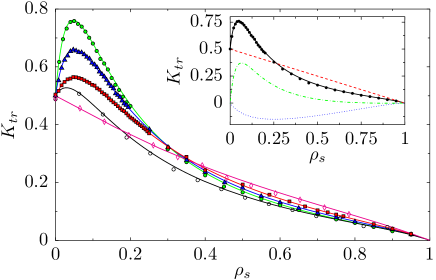
Figure 2: Dispersion coefficient as a function of the density $\rho_{s}$. Analytical expression (solid lines) vs numerical simulations (symbols) for different biases (filled symbols : $p_{1}=0.98$ ; empty symbols : $p_{1}=0.8$) and desorption rates $g$ ($\bullet$, $\circ$ : 0.15 ; $\blacktriangle$ : 0.2 ; $\blacksquare$ : 0.3 ; $\lozenge$ : 0.8). Inset : The different contributions to the dispersion coefficient, as defined in the main text, as a function of the density $\rho_{s}$ for $g=0.15$ : trivial mean-field (dashed), density (dotted), and cross-correlation (dashdotted) contributions. The sum of these contributions is the dispersion coefficient (analytical expression represented by a solid line vs numerical simulations denoted by symbols).

First, in the important limiting situation where no external driving is applied to the system, we find that

$$K_{tr}(E=0)=\frac{\frac{\sigma^{2}(1-\rho_{s})}{2\tau}}{1+\frac{\rho_{s}\tau^{*}}{\tau(f+g)}\frac{2}{1+\sqrt{1+2(1+\tau^{*}(1-\rho_{s})/\tau)/(f+g)}}}.$$

Beyond its own interest, this expression together with the approximate expression for the velocity obtained in Bénichou et al. (1999) in the linear driving regime using the decoupling approximation (6) shows that the Einstein relation (exact for the system under study Komorowski and Olla (2005)) is satisfied under the decoupling approximations, Eqs. (6) and (7). In other words, the approximations (6) and (7) are compatible with each other, which is a further validation of their applicability.

Second, in the high density limit, $\rho_{s}\to 1$, the dispersion coefficient obeys

$$K_{tr}\mathrel{\mathop{\kern 0.0pt\sim}\limits_{\rho_{s}\to 1}}\frac{\sigma^{2}}{2\tau}\frac{f+\sqrt{f(f+2)}}{f+\sqrt{f(f+2)}+2\tau^{*}/\tau}(1-\rho_{s}).$$ (18)

At leading order in $1-\rho_{s}$, $K_{tr}$ is thus independent of the amplitude of the driving force. Quite unexpectedly, it turns out that the dependence on the driving force of the density and of the correlation contributions to the dispersion coefficient exactly compensate each other in this limit.

Last, our analytical expression shows that, strikingly, $K_{tr}$ is a non-monotonic function of the density $\rho_{s}$, for values of $g$ smaller than some critical value $g_{c}$, and has a marked maximum at a certain value of $\rho_{s}$ (see figure 2). This result is a bit counter-intuitive, since one naturally expects that the dispersion will be maximal when there are no hard-core bath particles (i.e., when $\rho_{s}=0$).

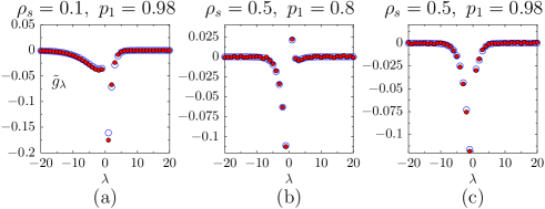
Figure 3: Cross-correlation functions $\tilde{g}_{\lambda}$ as a function of the distance to the tracer $\lambda$ for different values of the density $\rho_{s}$ and of the bias $p_{1}$. Analytical expressions (empty symbols) vs numerical simulations (filled symbols). (a) $f=0.033$, $g=0.3$ ; (b) and (c) $f=0.3$, $g=0.3$.

To gain some insight into this non trivial behavior, we represent (see inset of fig 2) three different contributions to the dispersion coefficient defined above (trivial mean-field, density, and cross-correlation contributions). As can be immediately seen, the non monotonic behavior of the variance originates from the non-monotonic behavior with $\rho_{s}$ of the cross-correlation function $\widetilde{g}_{1}$ in front of the tracer. These cross-correlations functions $\widetilde{g}_{\lambda}$, which provide a quantitative measure of the correlations between the fluctuations of the tracer position and the occupation numbers of the bath particles, are thus crucial in the problem. Actually, they display other non trivial and important behaviours (see fig. 3) revealed by our analytical expressions.

We first stress that the sign itself of these quantities is not trivial. While the analytical expressions allow us to show that, past the tracer, $\widetilde{g}_{\lambda}$ is always negative and corresponds to an anti-correlation of the fluctuations, it is found that $\widetilde{g}_{1}$ is positive in the high density limit

$$\widetilde{g}_{1}\mathrel{\mathop{\kern 0.0pt\sim}\limits_{\rho_{s}\to 1}}\frac{2p_{-1}\sigma(1-\rho_{s})}{2+[f+\sqrt{f(2+f)}]\tau/\tau^{*}}>0$$ (19)

or in the absence of a driving force

$$\widetilde{g}_{1}(E=0)\sim\frac{\sigma(1-\rho_{s})}{2}-\frac{\tau}{\sigma}K_{tr}(E=0)>0$$ (20)

where $K_{tr}(E=0)$ is given by Eq.(V), but can change sign otherwise. In other words, depending on the amplitude of the driving force and the density of the bath particles, positive or negative correlations between the fluctuations of the tracer position and the occupation numbers of the bath particles can take place. In addition, the monotonicity with the distance of these cross-correlation functions is also non-trivial – past (see fig. 3(a)) and in front of (see fig. 3(b)) the tracer – which further mirrors the complexity of these correlations.

VI Conclusion

In conclusion, we have studied the dynamics of a driven tracer in a bath of hard-core particles in the presence of adsorption/desorption processes. For this minimal model of active microrheology, we have developed an analytical framework to go beyond the standard force-velocity relation and quantitatively analyzed the fluctuations of the position of the tracer and their correlations with the occupation number of the bath particles at any position, for any density of the bath particles. This approach allowed us to obtain an exact Einstein-type relation between these correlations in the absence of a driving force and the density profiles of the bath particles in the linear driving regime. In the one-dimensional case we also provided an approximate but accurate explicit expression of the variance of the position of the tracer and shown in particular that it can behave non-monotically with the density of bath particles: counter-intuitively, increasing the density of hard-core particles can significantly increase the dispersion of the tracer position. We have shown that subtle correlations between the tracer position and the occupation of the bath particles past and in front of the tracer are responsible for this non trivial behavior. Altogether, our results put forward cross correlations as observables to analyze active microrheology data and predict a striking non monotonic behavior of the variance of the position of the tracer with respect to the density of the bath, that could in principle be observed experimentally. In a broader context, Equations (8) to (LABEL:systemeg2) together with Eqs.(2) and (3) provide a general framework to investigate important extensions that include the determination of explicit solutions in higher dimensions, in confined geometries and in non-stationary regimes.

Appendix A Master equation

Let $\eta\equiv\{\eta_{\bf R}\}$ denote the entire set of the occupation variables, which defines the instantaneous configuration of the adsorbed particles at the lattice at time moment $t$. Next, let $P({\bf R}_{tr},\eta;t)$ stand for the joint probability of finding at time $t$ the TP at the site ${\bf R}_{tr}$ and all adsorbed particles in the configuration $\eta$. Then, denoting as $\eta^{{\bf r},\nu}$ a configuration obtained from $\eta$ by the Kawasaki-type exchange of the occupation variables of two neighboring sites ${\bf r}$ and ${\bf r+e}_{\nu}$, and as ${\hat{\eta}}^{\bf r}$ a configuration obtained from the original $\eta$ by the replacement $\eta_{\bf r}\to 1-\eta_{\bf r}$, which corresponds to the Glauber-type flip of the occupation variable due to the adsorption/desorption events, we have that the time evolution of the configuration probability $P({\bf R}_{tr},\eta;t)$ obeys the following master equation :

$$2d\tau^{*}\partial_{t}P({\bf R}_{tr},\eta;t)=$$

$$\sum_{\mu=1}^{d}\;\sum_{{\bf r}\neq{\bf R}_{tr}-{\bf e}_{\mu},{\bf R}_{tr}}\;\Big{\{}P({\bf R}_{tr},\eta^{{\bf r},\mu};t)-P({\bf R}_{tr},\eta;t)\Big{\}}$$

$$+\frac{2d\tau^{*}}{\tau}\sum_{\mu}p_{\mu}\Big{\{}\left(1-\eta_{{\bf R}_{tr}}\right)P({\bf R}_{tr}-{\bf e}_{\mu},\eta;t)$$

$$-\left(1-\eta_{{\bf R}_{tr}+{\bf e}_{\mu}}\right)P({\bf R}_{tr},\eta;t)\Big{\}}$$

$$+2dg\sum_{{\bf r}\neq{\bf R}_{tr}}\;\Big{\{}\left(1-\eta_{\bf r}\right)P({\bf R}_{tr},\hat{\eta}^{{\bf r}};t)-\eta_{\bf r}P({\bf R}_{tr},\eta;t)\Big{\}}$$

$$+2df\sum_{{\bf r}\neq{\bf R}_{tr}}\;\Big{\{}\eta_{\bf r}P({\bf R}_{tr},\hat{\eta}^{{\bf r}};t)-\left(1-\eta_{\bf r}\right)P({\bf R}_{tr},\eta;t)\Big{\}}.$$

(21)

Note that the time evolution of the first moment $\langle X_{tr}(t)\rangle$ (Eq. 2) can be obtained by multiplying both sides of Eq. (21) by $({\bf R}_{tr}\cdot{\bf e}_{1})$ and summing over all possible configurations $({\bf R}_{tr},\eta)$.

Eqs. 8 and 12 (respectively 9 and LABEL:systemeg2) are obtained by multiplying both sides of Eq. (21) by $\eta({\bf R}_{tr}+{\bm{\lambda}})$ (respectively $X_{tr}\eta({\bf R}_{tr}+{\bm{\lambda}})$), summing over all possible configurations, and using the approximation 6 (respectively 7).

Appendix B Explicit expression of $K_{tr}$

B.1 Determination of $k_{1}$ and $k_{-1}$

According to Eq. 3, and defining $K_{tr}=\lim_{t\to\infty}\langle\delta X_{tr}^{2}\rangle/2t$,

$$K_{tr}=\frac{\sigma^{2}}{2\tau}(1-\rho_{s})-\frac{\sigma^{2}}{2\tau}\left[p_{1}(k_{1}-\rho_{s})\right.$$

$$\left.+p_{-1}(k_{-1}-\rho_{s})\right]-\frac{\sigma}{\tau}\left(p_{1}\widetilde{g}_{1}-p_{-1}\widetilde{g}_{-1}\right).$$

Thus, the computation of $k_{\pm 1}$ and $\tilde{g}_{\pm 1}$ from Eqs. 8, 12, 9, and LABEL:systemeg2 gives the expression of $K_{tr}$.

For one-dimensional lattices, a general solution of Eqs. 8 and 12 has the following form:

$$k_{n}\equiv k(\lambda)=\begin{cases}\rho_{s}+K_{+}r_{1}^{n}&\text{for $n>0$},\\ \rho_{s}+K_{-}r_{2}^{n}&\text{for $n<0$}.\end{cases}$$ (23)

where

$$r_{\begin{subarray}{c}2\\ 1\end{subarray}} = \frac{1}{2A_{1}}\bigg{(}A_{1}+A_{-1}+2(f+g)$$

$$\pm \left.\sqrt{\Big{(}A_{1}+A_{-1}+2(f+g)\Big{)}^{2}-4A_{1}A_{-1}}\right),$$

while the amplitudes $K_{\pm}$ are given respectively by

$$K_{+} = \rho_{s}\frac{A_{1}-A_{-1}}{A_{-1}-A_{1}r_{1}},$$ (25)

$$K_{-} = \rho_{s}\frac{A_{1}-A_{-1}}{A_{-1}/r_{2}-A_{1}}.$$ (26)

Now, we are in position to obtain a system of two closed-form non-linear equations determining implicitly the unknown parameters $A_{1}$ and $A_{-1}$, which will allow us to compute $k_{1}$ and $k_{-1}$. Substituting Eqs. 23, 25 and 26 into Eq. 11, we find

$$A_{1} = 1+\frac{2p_{1}\tau^{*}}{\tau}\Big{[}1-\rho_{s}-\rho_{s}\frac{A_{1}-A_{-1}}{A_{-1}/r_{1}-A_{1}},\Big{]}$$ (27)

$$A_{-1} = 1+\frac{2p_{-1}\tau^{*}}{\tau}\Big{[}1-\rho_{s}-\rho_{s}\frac{A_{1}-A_{-1}}{A_{-1}-A_{1}r_{2}}\Big{]}.$$ (28)

B.2 Determination of $\tilde{g}_{1}$ and $\tilde{g}_{-1}$

Using Eqs. 9 and LABEL:systemeg2 and the expressions 23 of $k_{n}$, the general equations satisfied by $\widetilde{g}$ become

$$A_{1}(\widetilde{g}_{n+1}-\widetilde{g}_{n})+A_{-1}(\widetilde{g}_{n-1}-\widetilde{g}_{n})-2(f+g)\widetilde{g}_{n}$$

$$+ \frac{2\tau^{*}}{\tau}\sigma\left\{p_{1}K_{+}r_{1}^{n}\left(1-\rho_{s}-K_{+}r_{1}-\frac{\widetilde{g}_{1}}{\sigma}\right)(r_{1}-1)\right.$$

$$- \left.p_{-1}K_{+}r_{1}^{n}\left(1-\rho_{s}-K_{+}r_{1}+\frac{\widetilde{g}_{-1}}{\sigma}\right)(r_{1}^{-1}-1)\right\}=0$$

for $n>1$,

$$A_{1}(\widetilde{g}_{n+1}-\widetilde{g}_{n})+A_{-1}(\widetilde{g}_{n-1}-\widetilde{g}_{n})-2(f+g)\widetilde{g}_{n}$$

$$+ \frac{2\tau^{*}}{\tau}\sigma\left\{p_{1}K_{-}r_{2}^{n}\left(1-\rho_{s}-K_{+}r_{1}-\frac{\widetilde{g}_{1}}{\sigma}\right)(r_{2}-1)\right.$$

$$- \left.p_{-1}K_{-}r_{2}^{n}\left(1-\rho_{s}-K_{+}r_{1}+\frac{\widetilde{g}_{-1}}{\sigma}\right)(r_{2}^{-1}-1)\right\}=0$$

for $n<-1$,

$$A_{1}\widetilde{g}_{2}-\widetilde{g}_{1}\left(A_{-1}+2(f+g)+\frac{2\tau^{*}}{\tau}p_{1}(\rho_{s}+K_{+}r_{1}^{2})\right)$$ (31)

$$+ \frac{2\tau^{*}}{\tau}p_{-1}(\rho_{s}+K_{+}r_{1})\widetilde{g}_{-1}$$

$$= -\frac{2\tau^{*}}{\tau}\sigma p_{1}(1-\rho_{s}-K_{+}r_{1})(\rho_{s}+K_{+}r_{1}^{2})$$

$$+ \frac{2\tau^{*}}{\tau}\sigma[p_{1}(1-\rho_{s}-K_{+}r_{1})$$

$$- p_{-1}(1-\rho_{s}-K_{-}r_{2}^{-1})](\rho_{s}+K_{+}r_{1}),$$

and

$$A_{-1}\widetilde{g}_{-2}-\widetilde{g}_{-1}\left(A_{1}+2(f+g)+\frac{2\tau^{*}}{\tau}p_{-1}(\rho_{s}+K_{-}r_{2}^{-2})\right)$$

$$+ \frac{2\tau^{*}}{\tau}p_{1}(\rho_{s}+K_{-}r_{2}^{-1})\widetilde{g}_{1}$$

$$= \frac{2\tau^{*}}{\tau}\sigma p_{-1}(1-\rho_{s}-K_{-}r_{2}^{-1})(\rho_{s}+K_{-}r_{2}^{-2})$$

$$+ \frac{2\tau^{*}}{\tau}\sigma[p_{1}(1-\rho_{s}-K_{+}r_{1})$$

$$- p_{-1}(1-\rho_{s}-K_{-}r_{2}^{-1})](\rho_{s}+K_{-}r_{2}^{-1}).$$

The general solution is written

$$\widetilde{g}_{n}=\begin{cases}\alpha r_{1}^{n}-\dfrac{V}{A_{1}r_{1}-A_{-1}r_{1}^{-1}}nr_{1}^{n}&\text{for $n>0$},\\ \beta r_{2}^{n}-\dfrac{W}{A_{1}r_{2}-A_{-1}r_{2}^{-1}}nr_{2}^{n}&\text{for $n<0$}.\end{cases}$$ (33)

where $\alpha$ and $\beta$ are constants to be determined,

$$V \equiv K_{+}\frac{2\tau^{*}}{\tau}\sigma\left\{p_{1}\left(1-\rho_{s}-K_{+}r_{1}-\frac{\widetilde{g}_{1}}{\sigma}\right)(r_{1}-1)\right.$$ (34)

$$- \left.p_{-1}\left(1-\rho_{s}-K_{+}r_{1}+\frac{\widetilde{g}_{-1}}{\sigma}\right)(r_{1}^{-1}-1)\right\}$$

and

$$W \equiv K_{-}\frac{2\tau^{*}}{\tau}\sigma\left\{p_{1}\left(1-\rho_{s}-K_{+}r_{1}-\frac{\widetilde{g}_{1}}{\sigma}\right)(r_{2}-1)\right.$$ (35)

$$- \left.p_{-1}\left(1-\rho_{s}-K_{+}r_{1}+\frac{\widetilde{g}_{-1}}{\sigma}\right)(r_{2}^{-1}-1)\right\}.$$

Substituting Eq. 33 into Eqs. 31 and B.2 on the one hand, and writing Eq. 33 for $n=1$ and $n=-1$ on the other hand, leads to a linear system of four equations satisfied by the four unknowns $\alpha$, $\beta$, $\widetilde{g}_{1}$ and $\widetilde{g}_{-1}$. It is finally found that:

$$\widetilde{g}_{1}=\frac{CE-BF}{AE-BD}\;\;{\rm and}\;\;\widetilde{g}_{-1}=\frac{AF-CD}{AE-BD},$$ (36)

where

$$A \equiv \frac{2\tau^{*}}{\tau}\sigma p_{1}K_{+}(r_{1}-1)\frac{A_{1}r_{1}^{2}}{A_{1}r_{1}-A_{-1}r_{1}^{-1}}+A_{1}r_{1}$$ (37)

$$- \left(A_{-1}+2(f+g)+\frac{2\tau^{*}}{\tau}p_{1}(\rho_{s}+K_{+}r_{1}^{2})\right),$$

$$B \equiv \frac{2\tau^{*}}{\tau}\sigma p_{-1}K_{+}(r_{1}^{-1}-1)\frac{A_{1}r_{1}^{2}}{A_{1}r_{1}-A_{-1}r_{1}^{-1}}$$ (38)

$$+ \frac{2\tau^{*}}{\tau}p_{-1}(\rho_{s}+K_{+}r_{1}),$$

$$C \equiv \frac{2\tau^{*}}{\tau}\sigma(p_{1}(1-\rho_{s}-K_{+}r_{1})$$

$$- p_{-1}(1-\rho_{s}-K_{-}r_{2}^{-1}))(\rho_{s}+K_{+}r_{1})$$

$$- \frac{2\tau^{*}}{\tau}\sigma p_{1}(1-\rho_{s}-K_{+}r_{1})(\rho_{s}+K_{+}r_{1}^{2})$$

$$+ \frac{2\tau^{*}}{\tau}\sigma\bigg{[}p_{1}(1-\rho_{s}-K_{+}r_{1})K_{+}r_{1}$$

$$- \left.p_{-1}\left(1-\rho_{s}-\frac{K_{-}}{r_{2}}\right)\frac{K_{+}}{r_{1}}\right]\frac{A_{1}r_{1}^{2}}{A_{1}r_{1}-A_{-1}r_{1}^{-1}},$$

$$D \equiv -\frac{2\tau^{*}}{\tau}\sigma p_{1}K_{-}(r_{2}-1)\frac{A_{-1}r_{2}^{-2}}{A_{1}r_{2}-A_{-1}r_{2}^{-1}}$$ (40)

$$+ \frac{2\tau^{*}}{\tau}p_{1}(\rho_{s}+K_{-}r_{2}^{-1}),$$

$$E \equiv -\frac{2\tau^{*}}{\tau}\sigma p_{-1}K_{-}(r_{2}^{-1}-1)\frac{A_{-1}r_{2}^{-2}}{A_{1}r_{2}-A_{-1}r_{2}^{-1}}+A_{-1}r_{2}^{-1}$$ (41)

$$- \left(A_{1}+2(f+g)+\frac{2\tau^{*}}{\tau}p_{-1}(\rho_{s}+K_{-}r_{2}^{-2})\right)$$

and

$$F \equiv \frac{2\tau^{*}}{\tau}\sigma(p_{1}(1-\rho_{s}-K_{+}r_{1})$$

$$- p_{-1}(1-\rho_{s}-K_{-}r_{2}^{-1}))(\rho_{s}+K_{-}r_{2}^{-1})$$

$$+ \frac{2\tau^{*}}{\tau}\sigma p_{-1}(1-\rho_{s}-K_{-}r_{2}^{-1})(\rho_{s}+K_{-}r_{2}^{-2})$$

$$- \frac{2\tau^{*}}{\tau}\sigma\bigg{[}(p_{1}(1-\rho_{s}-K_{+}r_{1})K_{-}r_{2}$$

$$- \left.p_{-1}\left(1-\rho_{s}-\frac{K_{-}}{r_{2}}\right)\frac{K_{-}}{r_{2}}\right]\frac{A_{-1}r_{2}^{-2}}{A_{1}r_{2}-A_{-1}r_{2}^{-1}},$$

where $K_{+}$, $K_{-}$, $A_{1}$, and $A_{-1}$ have been determined in the previous section.

References

• Wilson and Poon (2011) L. G. Wilson and W. C. K. Poon, PhysChemChemPhys 13, 10617 (2011).
• Wilson et al. (2011) L. G. Wilson, A. W. Harrison, W. C. K. Poon, and A. M. Puertas, Europhys. Lett. 93, 58007 (2011).
• Winter et al. (2012) D. Winter, J. Horbach, P. Virnau, and K. Binder, Phys. Rev. Lett. 108, 028303 (2012).
• Schroer and Heuer (2012) C. F. E. Schroer and A. Heuer, Phys. Rev. Lett. 110, 067801 (2013).
• Bénichou et al. (2012) O. Bénichou, C. Mejía-Monasterio, and G. Oshanin, Phys. Rev. E 87, 020103 (2013).
• Harrer et al. (2012) C. J. Harrer, D. Winter, J. Horbach, M. Fuchs, and T. Voigtmann, J. Phys.: Condens. Matter 24, 464105 (2012).
• Marini Bettolo Marconi et al. (2008) U. Marini Bettolo Marconi, A. Puglisi, L. Rondoni, and A. Vulpiani, Phys. Rep. 461, 111 (2008).
• Cugliandolo (2011) L. F. Cugliandolo, J. Phys. A 44, 483001 (2011).
• Gradenigo et al. (2012) G. Gradenigo, A. Puglisi, A. Sarracino, D. Villamaina, and A. Vulpiani, Out-of-equilibrium generalized fluctuation-dissipation relations (Chapter in the book: R.Klages, W.Just, C.Jarzynski (Eds.), Nonequilibrium Statistical Physics of Small Systems: Fluctuation Relations and Beyond (Wiley-VCH, Weinheim, 2012; ISBN 978-3-527-41094-1), 2012).
• Lizana et al. (2010) L. Lizana, T. Ambjörnsson, A. Taloni, E. Barkai, and M. A. Lomholt, Phys. Rev. E 81, 051118 (2010).
• Harris (1965) T. E. Harris, J. of Appl. Prob. 2, 323 (1965).
• Druger et al. (1983) S. D. Druger, A. Nitzan, and M. A. Ratner, J. Chem. Phys. 79, 3133 (1983).
• Bénichou et al. (2000a) O. Bénichou, J. Klafter, M. Moreau, and G. Oshanin, Phys. Rev. E 62, 3327 (2000a).
• Chou et al. (2011) T. Chou, K. Mallick, and R. K. P. Zia, Rep. on Prog. in Phys. 74, 116601 (2011).
• Parmeggiani et al. (2003) A. Parmeggiani, T. Franosch, and E. Frey, Phys. Rev. Lett. 90, 086601 (2003).
• Burlatsky et al. (1992) S. F. Burlatsky, G. Oshanin, A. Mogutov, and M. Moreau, Phys. Lett. A 166, 230 (1992).
• Burlatsky et al. (1996) S. F. Burlatsky, G. Oshanin, M. Moreau, and W. P. Reinhardt, Phys. Rev. E 54, 3165 (1996).
• Bénichou et al. (1999) O. Bénichou, A. M. Cazabat, A. Lemarchand, M. Moreau, and G. Oshanin, J. of Stat. Phys. 97, 351 (1999).
• Bénichou et al. (2000b) O. Bénichou, A. Cazabat, J. De Coninck, M. Moreau, and G. Oshanin, Phys. Rev. Lett. 84, 511 (2000b).
• Bénichou et al. (2001) O. Bénichou, A. M. Cazabat, J. De Coninck, M. Moreau, and G. Oshanin, Phys. Rev. B 63, 235413 (2001).
• Landim et al. (1998) C. Landim, S. Olla, and S. B. Volchan, Commun. in Math. Phys. 192, 287 (1998).
• Komorowski and Olla (2005) T. Komorowski and S. Olla, J. Stat. Phys. 118, 407 (2005).