Universality and conformal non-invariance in self-affine rough surfaces

Abstract

We show numerically that the roughness and growth exponents of a wide range of rough surfaces, such as random deposition with relaxation (RDR), ballistic deposition (BD) and restricted solid-on-solid model (RSOS), are independent of the underlying regular (square, triangular, honeycomb) or random (Voronoi) lattices. In addition we show that the universality holds also at the level of statistical properties of the iso-height lines on different lattices. This universality is revealed by calculating the fractal dimension, loop correlation exponent and the length distribution exponent of the individual contours. We also indicate that the hyperscaling relations are valid for the iso-height lines of all the studied Gaussian and non-Gaussian self-affine rough surfaces. Finally using the direct method of Langlands et.al we show that the contour lines of the rough surfaces are not conformally invariant except when we have simple Gaussian free field theory with zero roughness exponent.

I Introduction

Many theoretical and numerical efforts have been focused on the study, characterization, and understanding of stochastic surface patterns, for various growth models relevant to non-equilibrium processes Vicsek ; Barabasi ; Meakin . The surface roughening phenomena have been intensively studied via various discrete models and continuum equations. Scaling properties have been observed in time and space fluctuations of these surfaces and such interfaces show self-similar or self-affine properties Meakin .

Various growth models are often characterized and classified by three exponents, the roughness exponent, $\alpha$, the dynamical exponent, $z$, and the growth exponent, $\beta$. Most of the work is thus devoted to identifying the different universality classes to which the models studied belong EW ; Family ; KPZ ; Meakin1 ; Halpin ; BD1 ; BD2 ; RSOS . For example various discrete growth models such as the ballistic deposition (BD) BD1 ; BD2 , Eden Family and the restricted solid-on-solid (RSOS) RSOS models were known to be described by the Kardar-Parisi-Zhang (KPZ) equation in one dimension KPZ . Random deposition with surface relaxation (RDR) is another important discrete growth model that can be described by the Edwards-Wilkinson (EW) equation EW .

One of the most popular methods for characterization of the rough surfaces is based on the concept of fractal properties of iso-height lines called contour lines. The contour plot consists of closed non-intersecting loops in the plane that connect points of equal heights. Several experimental and numerical studies obtained the characterization of the fractal properties of loop ensembles of (2+1)Dimensional self-affine rough surfaces such as glassy interfaces and turbulence kondev1 , (2+1)Dimensional fractional Brownian motion smvaez , discrete scale invariant rough surfaces ghasemi , KPZ surfaces Niry , the multi-fractal surfaces multi , experimental data coming from the AFM analysis of WO₃ surfaces rajabpour and also STM images of rough metal surfaces kondev2 . One of the most important finding in this direction is the dependence of the different exponents i.e. the fractal dimension of one contour, $D_{f}$, the length distribution exponent, $\tau$, and the loop correlation-function exponent, $x_{l}$, related to the contour lines of mono-fractal rough surfaces to the only universal parameter in the system, i.e. roughness (Hurst) exponent. This conjecture confirmed by many numerical simulations but there is no theoretical proof yet kondev2 .

Most of the discrete surface growth models in (2+1)Dimension have been simulated on the square lattice with periodic boundary conditions with the topology of the torus Barabasi . There are a few works devoted to the study of the dynamical scaling exponents of surface growth on substrates with fractal structures fracsub1 ; fracsub2 . Here we numerically study the discrete growth models including random deposition (RD), RDR, BD and RSOS on different two dimensional lattice types such as square ($\mathcal{S}$), honeycomb ($\mathcal{H}$), triangular )$\mathcal{T}$), and also Voronoi random structure ($\mathcal{V}$). We show that universality holds, independent of the lattice type. The dynamical exponents $\alpha$ and $\beta$ for the surface growth process and also the geometrical scaling exponents $D_{f}$, $x_{l}$ and $\tau$ for the contour lines of such surfaces are not affected by the change of the substrate’s lattice type.

Another method to study two dimensional critical systems is by Schramm-Loewner evolution (SLE_κ). It gives a powerful tool to classify all the conformally invariant curves in two dimensions, for review see Baur . Recently, some studies argued that scaling exponents of 2D systems i.e. zero-vorticity lines of Navier-Stokes turbulence turbulence and domain walls in statistical models Baur can be determined by the diffusivity constant $\kappa$. We will show that the contour loop ensemble of RDR model, independent of lattice structure is conformal invariant object and could be described by SLE₄. Our numerical calculations show that the contour lines of RSOS model are not conformal invariant objects, however they can still possibly be classified by the Loewner’s equation.

The structure of this paper is organized as follows: In the next section we will investigate the scaling relations for the discrete surface growth processes. Scaling behaviors and corresponding properties of contour lines are also presented in detail in this section. The numerical results to measure scaling exponents for the stochastic surfaces i.e. RD, RDR, BD and RSOS models on different lattice types are discussed in the third section. In this section we also identify geometrical properties of loop ensembles by means of conformal invariant test. In the last section we will summarize our studies and we draw some concluding remarks.

II Scaling of rough surfaces

There are many non-equilibrium surface growth processes which exhibit scaling properties. Different models with the same scaling exponents are grouped into universality classes characterized by the same value of the critical exponents. Two methods to get some information about the scaling properties of the surface growth processes are $i)$ the dynamic evolution of the aggregate interface and, $ii)$ iso-height lines of the surfaces in the saturation regime.

II.1 Dynamical scaling exponents

The simplest quantitative behavior of a given aggregate interface is its interface width $W(t,L)\equiv\sqrt{\big{\langle}\frac{1}{L^{d}}\sum_{i=1}^{L^{d}}(h_{i}(t)-\bar{h}(t))^{2}\big{\rangle}}$ where $\bar{h}(t)$ is spatial average of height at time $t$ and $h_{i}(t)$ is the local height variable at the site $i$. The averaged roughness over different configurations show scaling behaviors. The width is saturated as $W\propto t^{\beta}$ with growth exponent $\beta$ and $W\propto L^{\alpha}$ with roughness $\alpha$ for short time and long time limits, respectively. The scaling exponents $\alpha$ and $\beta$ are used to characterize a given universality class of surface growth process Barabasi . Another quantity that describes dynamic of the growing rough surfaces is the height-height correlation function $C(r,t)\equiv\langle\left[h(\mathbf{r}_{0}+\mathbf{r},t)-h(\mathbf{r}_{0},t)\right]^{2}\rangle$. The heights separated by the short distances $r\ll L$ are fully correlated and the correlation function scales as $C(r,t)\propto r^{2\alpha}$ Barabasi .

II.2 Geometrical scaling exponents

For a given scale invariant height configuration $h(\mathbf{r})$, at the level cut at the mean height $h(\mathbf{r})=h_{0}$, there are many closed non-intersecting contour loops that connect points of equal height. A few scaling functions and scaling exponents need to characterize the size distribution of such contour lines. Contour loops with length $s$ and radius $R$ are scale invariant and follows a power law $\langle s\rangle\sim\langle R\rangle^{D_{f}}$, where $D_{f}$ is the fractal dimension of a contour loop. The contour line properties can be described by the probability distribution of contour lengths $\tilde{P}(s)$. This function measures the probability that one loop has length $s$ and it follows the scaling behavior $\tilde{P}(s)\sim s^{-\tau}$ where $\tau$ is a scaling exponent. Another interesting quantity with the scaling property is the loop correlation function $G_{c}(\mathbf{r})$. This function is a probability measure for the two points in the plane where separated by the distance $|\mathbf{r}|$ lie on the same contour. For iso-height lines on the grid with lattice constant $\mathbf{c}$ and in the limit $|\mathbf{r}|\gg\mathbf{c}$, the two point correlation function is also scale invariant $G_{c}(\mathbf{r})\sim\frac{1}{|\mathbf{r}|^{2x_{l}}}$, where $x_{l}$ is the loop correlation-function exponent. For the contour loops on a Gaussian surface, $x_{l}=\frac{1}{2}$ is conjectured kondev3 . There is no any mathematical proof for this hypothesis yet. The estimated value $x_{l}=\frac{1}{2}$ is confirmed by various numerical works for large class of the known self-affine rough surfaces kondev1 ; ghasemi ; kondev2 .

For the Gaussian self-affine rough surfaces with the roughness exponent $\alpha$ and the scaling exponents $D_{f}$, $\tau$ and $x_{l}$, it was shown that the two well known hyper-scaling relations

$$D_{f}(\tau-1)=2-\alpha,\hskip 28.45274ptD_{f}(\tau-3)=2x_{l}-2,$$ (1)

are valid kondev2 . Finally there is another measure associated with a given contour loop ensemble which is called the two point correlation function for contour lines with length $s$, $G_{s}$. Scaling properties of the contours force $G_{s}(r)$ to scale with $s$ and $r$ as $G_{s}(\mathbf{r})\sim s^{m}|\mathbf{r}|^{-n}f_{G_{s}}(\frac{r}{R})$ where the new exponents satisfy kondev1

$$2-n=D_{f}(1-m).$$ (2)

In the next section we numerically calculate all introduced exponents $\alpha$, $\beta$, $D_{f}$, $\tau$, $x_{l}$, $n$ and $m$ for RD, RDR, BD and RSOS on different lattice structures and we will show the validity of the two scaling relations in Eq. (1) and also the Eq. (2).

III Numerical results

The lattice version of RD, RDR, BD and RSOS models are simple to describe. In all of them particles fall on vertical direct line onto the substrate from a random position above the surface Barabasi . In the simple on-top site RD model, the particle deposits on randomly chosen site position. In RDR model a particle is released on the top of a selected column, but it does not stick to the surface immediately and it can diffuse to a nearest neighbor site of lower height Barabasi ; EW . Surface diffusion generates correlation between neighbor sites and it causes surface width saturation effect. In BD model, falling particle sticks to the old one either on the top or a nearest neighbor occupied site Barabasi ; BD1 ; BD2 . In RSOS surface growth process the particle aggregates to the substrate if and only if the difference between heights of all pairs of nearest-neighbor columns satisfies the condition $\Delta h\leq 1$; otherwise, if this condition is not met, the corresponding aggregation attempt is rejected from the system RSOS .

In order to find dynamical and geometrical scaling properties of RD, RDR, BD and RSOS models on the initially flat substrates, we have generated these models on different lattice types, i.e. honeycomb, triangular, square and Voronoi with size $L=512$ and all measurements are made using an ensemble of 2000 realizations (for BD model the simulation were also done on lattices with size $L=2048$ with 500 samples). In order to reduce the errors due to the substrate’s boundaries, we used periodic boundary condition during particle deposition in horizontal and vertical directions. Each time step is defined as the number of particles to fall up surface on the average, which is equal to $L\times L$. To extract the contour lines of the saturated surfaces at the mean height, $h_{0}$ we used Hoshen-Kopelman algorithm HK .

III.1 Distribution of heights

To check that the surface that we have is a Gaussian surface or not we used the definition of local curvature at $\mathbf{r}$ and at scale $b$ which is kondev3

$$C_{b}(\mathbf{r})\equiv\sum_{m=1}^{M}\left[h(\mathbf{r}+b\mathbb{e}_{m})-h(\mathbf{r})\right]$$ (3)

where the sum of $\mathbb{e}_{m}$’s are a fixed set of vectors summing to zero. The distribution of the local curvature in Gaussian surfaces is Gaussian. In Fig.  1 one can see that the distribution is Gaussian for RDR but non-Gaussian for RDR and BD. To quantify this claim we depicted in Fig.  2 the third $\frac{\langle C_{b}(\mathbf{r})^{3}\rangle}{\langle C_{b}(\mathbf{r})^{2}\rangle^{3/2}}$ and fourth moments $\frac{\langle C_{b}(\mathbf{r})^{4}\rangle}{\langle C_{b}(\mathbf{r})^{2}\rangle^{2}}$ of the local curvature which should be $0$ and $3$ for a Gaussian surfaces respectively. Based on these two figures we conclude that among the surfaces that we are going to study just the RDR is a Gaussian surface. It is worth mentioning that by increasing the scale $b$, the results of RDR and BD surface growth models converge to the Gaussian process. We also repeated these computations for the other lattice types and the results are the same as that of for square lattice type. Finally we also checked the self-affinity of our surfaces by showing that for all the surfaces we have $\langle[C_{b}(\mathbf{r})]^{q}\rangle\sim b^{q\alpha}$.

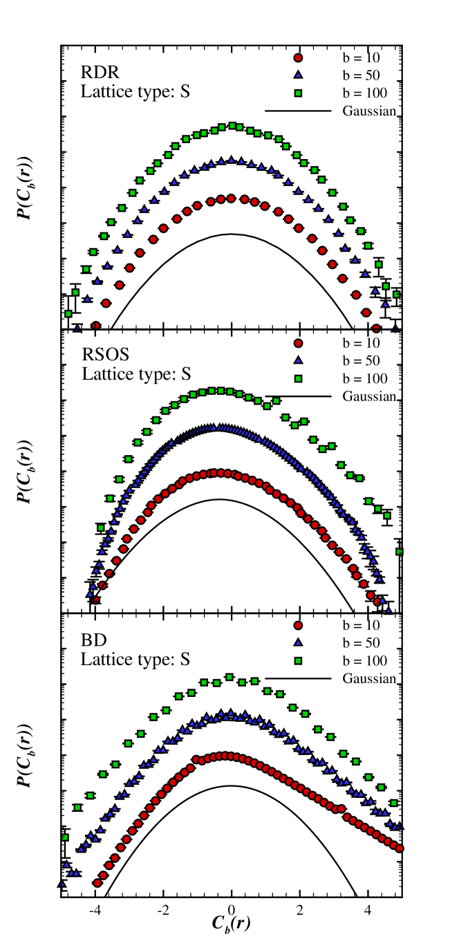
Figure 1: (Color online) The distribution of the local curvature in RDR, BD and RSOS model. To make more sense we shifted various plots vertically.

Figure 2: (Color online) The third and fourth moments of the local curvature in RDR, BD and RSOS models on square lattice type.

III.2 Scaling exponents

One approach to show that two rough surface models belong to the same universality class is to compute all scaling exponents of the models. In this sub-section we report measured values of the scaling exponent for various models.

• The growth scaling exponent

In Table. 1, we have shown the results for various growth models on different lattice types. Our measurements of the scaling exponent $\beta$ on the square lattice are consistent with previous studies Barabasi ; saberi .

Table 1: Numerical values of the scaling exponents $\beta$ for different surface growth models on the different lattices ($\mathcal{H}$: Honeycomb, $\mathcal{S}$: Square, $\mathcal{T}$: Triangular, $\mathcal{V}$:Voronoi). The numbers inside the parenthesis are the error bars of the last digits.

	Lattice type
Model	$\mathcal{H}$	$\mathcal{S}$	$\mathcal{T}$	$\mathcal{V}$
RD	$0.500(1)$	$0.500(1)$	$0.500(1)$	$0.500(1)$
RSOS	$0.240(2)$	$0.240(5)$	$0.240(5)$	$0.240(3)$
BD	$0.24(1)$	$0.24(1)$	$0.23(2)$	$0.24(1)$

Our result confirms logarithmic scaling of roughness $W(t,L)\sim\ln(t)$ for RDR model where is in agreement with the predictions Barabasi ; EW .

• Roughness exponent

To measure the roughness exponent $\alpha$ we have calculated the height-height correlation function $C(r)$ with respect to the distance separation $r$ for saturated time. Using numerical calculations for small values of $r$, the roughness exponent can be read where Table 2 reports all the measured values of the roughness exponent for BD and RSOS lattice growth models on different lattice types. Results from numerical computation of $\alpha$ for growth processes on the square lattice is in good agreement with the previously reported values Barabasi ; saberi .

Table 2: Numerical values of the scaling exponents $\alpha$ for BD and RSOS models on different lattice types.

	Lattice type
Model	$\mathcal{H}$	$\mathcal{S}$	$\mathcal{T}$	$\mathcal{V}$
RSOS	$0.400(2)$	$0.400(2)$	$0.400(3)$	$0.400(5)$
BD	$0.30(4)$	$0.29(4)$	$0.29(4)$	$0.30(4)$

For RDR model deposited on different lattice types, we observed $C(r)\sim\ln(r)$ Barabasi ; EW .

• Geometrical scaling exponents

Table 3: Numerical values of different geometrical exponents $x_{l}$, $D_{f}$ and $\tau-1$ at $1\sigma$ confidence interval for the discrete surface growth models on different lattices.

		Lattice type
		$\mathcal{H}$	$\mathcal{S}$	$\mathcal{T}$	$\mathcal{V}$
$2x_{l}$	RDR	$1.0(1)$	$1.0(1)$	$1.0(1)$	$1.0(1)$
	RSOS	$1.0(1)$	$1.0(1)$	$1.0(1)$	$1.0(1)$
	RD	$0.53(5)$	$0.47(5)$	$0.49(4)$	$0.52(5)$
	BD	$1.0(2)$	$1.0(2)$	$1.0(2)$	$1.0(2)$
$D_{f}$	RDR	$1.50(1)$	$1.50(1)$	$1.49(1)$	$1.49(2)$
	RSOS	$1.30(1)$	$1.30(1)$	$1.30(1)$	$1.30(1)$
	RD	$1.73(1)$	$1.73(1)$	$1.75(1)$	$1.73(1)$
	BD	$1.36(2)$	$1.36(2)$	$1.36(2)$	$1.36(2)$
$\tau-1$	RDR	$1.33(1)$	$1.34(1)$	$1.34(1)$	$1.33(1)$
	RSOS	$1.22(1)$	$1.23(1)$	$1.22(1)$	$1.22(1)$
	RD	$1.18(1)$	$1.19(1)$	$1.19(1)$	$1.19(1)$
	BD	$1.32(2)$	$1.31(2)$	$1.32(3)$	$1.32(2)$
$n$	RDR	$0.49(2)$	$0.50(2)$	$0.50(2)$	$0.51(2)$
	RSOS	$0.69(2)$	$0.69(2)$	$0.68(2)$	$0.69(2)$
	RD	$0.30(2)$	$0.29(2)$	$0.30(2)$	$0.31(2)$
	BD	$0.66(2)$	$0.67(3)$	$0.65(2)$	$0.66(2)$
$m$	RDR	$0.02(3)$	$0.02(2)$	$0.02(2)$	$0.02(2)$
	RSOS	$0.03(3)$	$0.03(3)$	$0.03(3)$	$0.02(3)$
	RD	$0.03(3)$	$0.02(3)$	$0.02(2)$	$0.03(3)$
	BD	$0.04(5)$	$0.04(4)$	$0.03(4)$	$0.03(3)$

The most important exponent in fractal contour lines is the loop correlation function exponent $x_{l}$. For a given loop ensemble we followed the algorithm reported in the Ref. kondev1 to find the correlation function $G_{c}(r)$. The first part of the Table .3 shows that the measured values for the exponent $x_{l}$ for discrete growth processes i.e. RDR model with the Gaussian statistics are in agreement with the predicted value $2x_{l}=1$, within the statistical error. According to our results, it is quite interesting that the relation $2x_{1}=1$ is valid also for non-Gaussian interfaces such as RSOS model. We observed $2x_{l}=\frac{1}{2}$ for the RD model which is in agreement with the predicted value for the two point correlation exponent of the percolation model lolo . The difference between RD model and the other growth processes comes from the correlation between lattice sites in the deposition process. There are no any correlations between nearest neighbor sites in the RD model. The same calculations are done for the BD model on different lattice types. The large error bars which lead to the less agreement in the equality $2x_{1}=1$ come from finite size effects. One can compute the perimeter, $s$, and gyration, $R$, radius of contour loops to calculate fractal dimension $D_{f}$. Here $R$ is defined by $R^{2}=\frac{1}{N}\sum_{i=1}^{N}\left[(x_{i}-x_{c})^{2}+(y_{i}-y_{c})^{2}\right]$, with $x_{c}=\frac{1}{N}\sum_{i=1}^{N}x_{i}$ and $y_{c}=\frac{1}{N}\sum_{i=1}^{N}y_{i}$. In the second part of the Table 3 we have shown the measured values of the fractal dimension of contour loops for all surface growth processes on different lattice types. The next remark concerns the probability distribution of contour length $\tilde{P}(s)$ with the scaling exponent $\tau$. We measured $\tau$ for different models, results are shown in the third part of Table .3. A suitable value of the parameter $\tau$ obtained form the best fit to $\ln(\tilde{P}(s))$ versus $\ln(s)$ (We measured $\tau-1$ instead of $\tau$). Finally we also calculated $G_{s}(r)$ and the exponents $m$ and $n$; the results are listed in Table .3.

• Scaling relations

Finally the relation between measured scaling exponents $\alpha$, $x_{l}$, $D_{f}$, $\tau$, $m$ and $n$ given by Eq. 1 and Eq. 2 can be examined. We have depicted the results for all growth models on different lattice types in the Table .4. As can be seen from the Tables. 1, 2 and 3 the error bars for the BD results are very large. It seems that to get conclusive results one needs to simulate the BD model on very large lattice sizes LargBD which is very time consuming. However, due to the finite size effect, we concluded that our results are roughly consistent with the predictions.

Table 4: Verification of three basic hyper-scaling relations for discrete surface growth process on different lattice types.

		$D_{f}(\tau-1)$	$2-\alpha$	$D_{f}(\tau-3)$	$2-2x_{l}$	$D_{f}(1-m)$	$2-n$
RD	$\mathcal{H}$	$2.04(3)$	$2$	$1.42(3)$	$1.47(5)$	$1.68(4)$	$1.70(2)$
	$\mathcal{S}$	$2.06(5)$	$2$	$1.40(5)$	$1.53(5)$	$1.69(4)$	$1.71(2)$
	$\mathcal{T}$	$2.08(6)$	$2$	$1.42(6)$	$1.51(4)$	$1.71(3)$	$1.70(2)$
	$\mathcal{V}$	$2.06(5)$	$2$	$1.40(5)$	$1.48(5)$	$1.68(4)$	$1.69(2)$
BD	$\mathcal{H}$	$1.79(6)$	$1.70(4)$	$0.93(4)$	$1.0(2)$	$1.30(6)$	$1.34(2)$
	$\mathcal{S}$	$1.78(8)$	$1.71(4)$	$0.94(6)$	$1.0(2)$	$1.30(6)$	$1.33(3)$
	$\mathcal{T}$	$1.79(6)$	$1.71(4)$	$0.93(4)$	$1.0(2)$	$1.32(6)$	$1.35(2)$
	$\mathcal{V}$	$1.79(6)$	$1.70(4)$	$0.93(4)$	$1.0(2)$	$1.32(5)$	$1.34(2)$
RDR	$\mathcal{H}$	$2.00(3)$	$2$	$1.01(3)$	$1.0(1)$	$1.47(4)$	$1.51(2)$
	$\mathcal{S}$	$2.01(3)$	$2$	$0.99(3)$	$1.0(1)$	$1.47(3)$	$1.50(2)$
	$\mathcal{T}$	$2.00(3)$	$2$	$0.98(3)$	$1.0(1)$	$1.46(3)$	$1.50(2)$
	$\mathcal{V}$	$1.98(4)$	$2$	$1.00(4)$	$1.0(1)$	$1.46(3)$	$1.49(2)$
RSOS	$\mathcal{H}$	$1.59(2)$	$1.60(1)$	$1.01(2)$	$1.0(1)$	$1.26(4)$	$1.31(2)$
	$\mathcal{S}$	$1.60(2)$	$1.60(1)$	$1.00(2)$	$1.0(1)$	$1.26(4)$	$1.31(2)$
	$\mathcal{T}$	$1.59(2)$	$1.60(1)$	$1.01(2)$	$1.0(1)$	$1.26(4)$	$1.32(2)$
	$\mathcal{V}$	$1.59(2)$	$1.60(1)$	$1.01(2)$	$1.0(1)$	$1.27(4)$	$1.31(2)$

III.3 Conformal invariance (CI) test

It is well-known, for a recent discussion see Rajabpour , that the action corresponding to Gaussian self-affine rough surfaces is conformally invariant just for the surfaces with zero roughness exponent. However, recently many authors claimed that despite the non-conformal invariant height ensembles of these surfaces, their contour lines might be conformally invariant turbulence2 ; Niry ; saberi . In the following we examine this guess by using the direct conformal invariance test used first in langlands1 . Suppose a conformal mapping defined by $w=g_{t}(z)$. For any domain $\mathcal{D}$ with boundary $\mathcal{C}$, one can find a conformal map $g_{t}$ where maps $\mathcal{D}$ to $\mathcal{D^{\prime}}$ and $\mathcal{C}$ to $\mathcal{C^{\prime}}$. For the critical statistical systems, the measure on distributions on $\mathcal{C^{\prime}}$ is obtained by transport of the measure on distributions on $\mathcal{C}$ using conformal mapping $g_{t}$ from $\mathcal{D}$ to $\mathcal{D^{\prime}}$ where this measure is invariant at the critical point of the model.

Statistical systems such as, percolation and Potts models at the critical point, exhibit a unique spanning cluster, where connect the boundaries of domain from one side to the other (i.e. left to right or up to down) along the spanning cluster stauffer . In the scaling limit when the size of the system goes to infinity, one can define the crossing probability $\pi_{h}$ ($\pi_{v}$), the probability of a system to percolate only in the horizontal (vertical) direction langlands1 . In the conformal invariant statistical systems, the measure $\pi_{h}$ ($\pi_{v}$) is unchanged under any conformal map $g_{t}$ where it maps a given boundary $\mathcal{C}$ to $\mathcal{C}^{\prime}$ langlands1 ; langlands2 ; langlands3 ; blanchard .

The conformally invariant curves should be statistically equivalent to Schramm Loewner evolution (SLE_κ). In this method the conformal map $g_{t}(z)$ which maps the half-plane minus the trace $\gamma_{t}$ into itself, obeys the Loewner’s formula $\partial_{t}g_{t}=2/{(g_{t}-\xi_{t})}$ where the driving function $\xi_{t}$ is related to the Brownian motion with the diffusivity $\kappa$. The fractal dimension of such scaling curves is given by the relation $d_{f}=1+\kappa/8$. In turbulence2 ; Niry ; saberi , using a discretized Loewner equation and iterative conformal slit map they extracted the drift $\xi_{t}$ for iso-height lines in the different rough surfaces. They found that an ensemble of the driving function $\xi_{t}$ for these models looks like converging to a Gaussian process with zero mean $\langle\xi_{t}\rangle\approx 0$ and the variance $\langle\xi_{t}^{2}\rangle\approx\kappa t$ with $\kappa$ compatible with the fractal dimension of the curves. It shows for example that the model with logarithmic height correlation can be related to SLE₄. However, it seems that the calculations based on Loewner evolution (using Schramm Loewner equation to find $\kappa$) are not accurate enough. Especially it is not easy to find the exact Gaussian distribution for the increments of the driving function and also it is difficult to show stationarity of increments of the drift to conclude that the drift is really a Brownian motion. For example even for RDR (which is a Gaussian free field) we know that usually the drift is not just a Brownian motion, it is a complicated function related to the Brownian motionGFF .

An alternative way is to apply directly the conformal invariant test to a two dimensional slice of random rough surface. For a given rough surface sample $h(x,y)$, a horizontal cut is made at a certain level $h_{c}=\langle h\rangle+\delta\sqrt{\langle[h-\langle h\rangle]^{2}\rangle}$, where the symbol $\langle...\rangle$ is averaging over ensemble of rough surfaces. A set of nearest-neighbor connected sites of positive (negative) height form a cluster. The cluster is spanning one if spans two opposite sides of a given domain, such that infinite connectivity first occurs, and one can measure the crossing probabilities $\pi_{h}(\delta)$ and $\pi_{v}(\delta)$ for a given domain geometry.

In this study we considered square boundary as $\mathcal{C}$ and rhombus domains with different angle as $\mathcal{C}^{\prime}$ . There is a conformal map that takes interior of our choice of $\mathcal{C}$ to the interior of $\mathcal{C}^{\prime}$ and takes vertices to vertices and sides to sides. The basic method to perform this test composed of three steps: (I) draw the boundary $\mathcal{C}$ ( $\mathcal{C^{\prime}}$) defining cluster ensemble on the lattice. (II) assign a state $+1$ ($-1$) to each site of the lattice located inside $\mathcal{C}$ ($\mathcal{C^{\prime}}$) when $h(x,y)>h_{c}$ ($h(x,y)\leq h_{c}$). (III) find cluster of nearest-neighbor connected sites with the same values (for example $+1$) by using Hoshenn-Kopelman (HK) algorithm HK . These three steps are repeated for all of the configurations of level set ensemble for various $\delta$’s to find the largest cluster where spans left and right, to measure $\pi_{h}$ (up and down to measure $\pi_{v}$). The expected value of $\pi_{h}$ ($\pi_{v}$), is then the ratio of the number of configurations spanning two opposite horizontal or vertical sides of the boundary $\mathcal{C}$ ( $\mathcal{C}^{\prime}$) to the sample size.

We examined the above test for two dimensional slice of RD, RDR, RSOS and also synthetic (2+1)Dimensional self-affine surfaces which known as fractional Brownian motion (2D FBM) smvaez for different $\delta$’s and we measured crossing probability $\pi_{h}(\delta)$ ($\pi_{v}(\delta)$) for different boundaries $\mathcal{C}$ (square with side length $L$) and $\mathcal{C}^{\prime}$ (rhombus with angle $\theta$ and side $L$). In order to have an ensemble of surface height profiles, we have obtained $2\times 10^{5}$ samples from the grown rough surfaces with side $L=512$ for each model. We measured the probabilities $\pi_{h}(\delta)$ and $\pi_{v}(\delta)$ that at each level height $\delta$, an infinite island spans two opposite boundaries of the domains.

As shown in Fig 3 the measured crossing probabilities for RDR model on rhombus domains with different angles $\theta$, cross each other at $\delta=\delta_{c}$, implying that the crossing probabilities remain constant by conformal transformation. This means that the two dimensional slices of RDR model at the critical level $\delta_{c}$ is possibly conformally invariant and the crossing probabilities do not change by conformal transformations. We also applied this test to 2D FBM with Hurst exponent $0\leq H\leq 1$ and we observed conformal invariance only for $H=0$. We observed that the 2D FBM with $H>0$ is conformal non-invariant and the spanning probability $\pi_{h}(\delta)$ do not show any fixed point. In addition we presented in Fig. 3 the curves $\pi_{h}(\delta)$ obtained for RSOS model on different boundaries. It shows that the crossing probability for two dimensional slice of RSOS model for different $\delta$’s, change by conformal transformation of the boundary. Increasing the number of ensembles and the size of the system did not make significant change in this pattern. We concluded that this model is also conformally non-invariant.

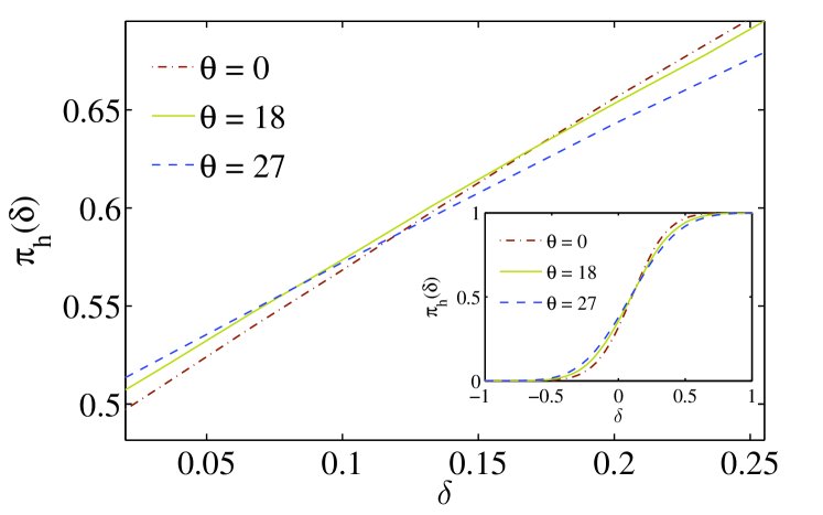
Figure 3: (Color online) The spanning probability $\pi_{h}(\delta)$ for two dimensional slice of RSOS model on rhombus domain with different angles $\theta$. Inset: The same quantity for RDR.

Our results show that the contour ensemble of RD model on the triangular lattice at the mean height ($\delta=0$) is conformally invariant. Two dimensional slice of RD model at the mean level for other lattice types is conformal non-invariant. This is obvious if we think to the clusters of RD as a simple percolation clusters. Our numerical results are summarized in Tabel. (5).

Table 5: CI test results of two dimensional loop ensembles of random rough surfaces.

	Lattice type
model	$\mathcal{S}$	$\mathcal{T}$
RD	No	Yes
RDR	Yes	Yes
RSOS	No	No
FBM$(H\neq 0)$	No	No

IV Conclusion

In this paper we showed that many properties of rough surfaces such as the roughness exponent and dynamical exponent are independent of the underlying lattices, see Table. 1 and 2. We also showed that the fractal dimension and correlation exponent and many other exponents of contour lines of the surfaces are also independent of the underlying lattices and the distribution of the heights. All the calculations were carried out on four different regular and irregular lattices such as the square, triangular, honeycomb and Voronoi lattices, see Table. 3. Although the calculations for BD were not conclusive we were able to show that the extracted critical exponents of the contour lines of RDR, RSOS and RD follow the hyperscaling relations independent of having a Gaussian or non-Gaussian surface, see Table. 4. Finally using direct conformal maps we showed that the contour lines of self-affine rough surfaces (RSOS, BD and fractional Gaussian rough surfaces) with non-zero roughness exponents are not conformally invariant. To be specific just the contour lines of RDR on different lattices and RD on the triangular lattices are conformally invariant, see Table. 5.

Acknowledgment: We thank M. Ghasemi Nezhadhaghighi for many discussions and helps. We also thank A Saberi and S Rouhani for reading the manuscript. The work of S. Hosseinabadi was supported by Islamic Azad University, East Tehran Branch. MAR thanks FAPESP for finantial support.

References

- (1) T. Vicsek , Fractal Growth Phenomena, World Scientific, Singapore (1992)
- (2) A. L. Barabsi and H.E. Stanley, Fractal Concepts in Surface Growth, Cambridge University Press: Cambridge (1995)
- (3) P. Meakin, Fractals, Scaling, and Growth Far From Equilibrium, Cambridge University Press: Cambridge (1998) and G. R. Jafari, S. M. Fazeli, F. Ghasemi, S. M. Vaez Allaei, M. Reza Rahimi Tabar, A. Iraji zad, G. Kavei, Phys. Rev. Lett, 91 (2003) 226101
- (4) S. F. Edwards and D. R. Wilkinson, Proc. Roy. Soc. London A, 381 (1982) 17 and A. Iraji zad, G. Kavei, M. Reza Rahimi Tabar, S.M. Vaez Allaei, J. Phys: Condens. Matter, 15 (2003) 1889
- (5) F. Family T. Vicsek, J. Phys. A, 18(1985) L75
- (6) M. Kardar, G. Parisi and Y. C. Zhang, Phys. Rev. Lett, 56 (1986) 889
- (7) P. Meakin, Phys. Rep, 235 (1993) 189
- (8) T. Halpin-Healy and Y.C. Zhang, Phys. Rep, 254(1995)215
- (9) P. Meakin, P. Ramanlal, L.M. Sander and R. C. Ball, Phys. Rev. A, 34 (1986) 5091
- (10) J. Krug and P. Meakin, Phys. Rev. A, 40 (1989) 2064
- (11) J. M. Kim and J. M. Kosterlitz, Phys. Rev. Lett, 62 (1989) 2289; F. D. A. A. Reis, Phys. Rev. E, 63(2001)056116; S. Hosseinabadi, A. A. Masoudi, M. Sadegh Movahed, Physica B: Condensed Matter, 405 (2010) 2072
- (12) C. Zeng, J. Kondev, D. McNamara and A. A. Middleton, Phys. Rev. Lett, 80 (1998)109; J. Kondev and G. Huber, Phys. Rev. Lett, 86(2001)26
- (13) M. A. Rajabpour and S. M. Vaez Allaei, Phys. Rev. E, 80(2009)011115 [arXiv:0907.0881]
- (14) M. G. Nezhadhaghighi and M. A. Rajabpour, Phys. Rev. E, 83(2011)021122 [arXiv:1011.1118]
- (15) A. A. Saberi, M. D. Niry , S. M. Fazeli, M. R. Rahimi Tabar and S. Rouhani, Phys. Rev. E, 77(2008)051607
- (16) S. Hosseinabadi, M. A. Rajabpour, M. Sadegh Movahed and S. M. Vaez Allaei, Physical Review E, 85(2012)031113 [arxiv:1107.5287v1]
- (17) A. A. Saberi, M. A. Rajabpour and S. Rouhani S, Phys. Rev. Lett, 100(2008)044504
- (18) J. Kondev and C. L. Henley, Phys. Rev. Lett, 74 (1995)4580; J. Kondev, C. L. Henley and D. G. Salinas, Phys. Rev. E, 61 (2000)104
- (19) C. M. Horowitz, F. Romá and V. Albano Ezequiel, Phys. Rev. E, 78(2008)061118
- (20) Sang Bub Lee et al, J. Stat. Mech (2008)P12013; Dae Ho Kim and Jin Min Kim, J. Stat. Mech (2010)P08008; Dae Ho Kim and Jin Min Kim, Phys Rev E, 84 (2011) 011105
- (21) M. Bauer and D. Bernard, Phys. Rep, 432(2006)115
- (22) D. Bernard, G. Boffetta, A. Celani and G. Falkovich, Nature Phys, 2(2006)124
- (23) J. J. Ramasco, J. M. Lopez and M. A. Rodriguez, Phys. Rev. Lett, 84(2000)2199
- (24) J. Kondev and C. L. Henley, Nuclear Physics B, 464(1996)540
- (25) J. Hoshen and R. Kopelman, Phys. Rev. B, 14(1976)3438
- (26) A. A. Saberi, H. Dashti-Naserabadi and S. Rouhani, Phys Rev E, 82(2010)020101
- (27) H. Saleur and B. Duplantier, Phys. Rev. Lett, 58(1987)2325 2328
- (28) B. Farnudi and D. D. Vvedensky, Phys Rev E, 83(2011)020103; C. Lehnen and T. M. Lu, Phys Rev B, 82(2010)085437
- (29) M. A. Rajabpour, JHEP, 06(2011)076 [arXiv:1103.3625]
- (30) D. Bernard, G. Boffetta, A. Celani and G. Falkovich, Phys. Rev. Lett, 98(2007)024501
- (31) R. P. Langlands, Ph. Pouliot and Y. Saint-Aubin, Bull. AMS, 30(1994)1
- (32) D. Stauffer and A. Aharony, Introduction to Percolation Theory Taylor Francis, London (1994)
- (33) R. P. Langlands, C. Pichet, Ph. Pouliot and Y. Saint-Aubin, J. Stat. Phys, 67(1992)553
- (34) R. P. Langlands, M-A. Lewis and Y. Saint-Aubin, J. Stat. Phys, 98(2000)131
- (35) Ph. Blanchard, S. Digal, S. Fortunato, D. Gandolfo, T. Mendes and H. Satz, J. Phys. A: Math. Gen, 33(2000)8603
- (36) O. Schramm and S. Sheffield, Acta Math, 202(2009)21