Generalized Projected Dynamics For Non-System Observables of Nonequilibrium Quantum Impurity Models

Abstract

The reduced dynamics formalism has recently emerged as a powerful tool to study the dynamics of nonequilibrium quantum impurity models in strongly correlated regimes. Examples include the nonequilibrium Anderson impurity model near the Kondo crossover temperature and the nonequilibrium Holstein model, for which the formalism provides an accurate description of the reduced density matrix of the system for a wide range of timescales. In this work, we generalize the formalism to allow for non-system observables such as the current between the impurity and leads. We show that the equation of motion for the reduced observable of interest can be closed with the equation of motion for the reduced density matrix and demonstrate the new formalism for a generic resonant level model.

I Introduction

The study of open quantum impurity models, where the coupling of a small system to multiple baths drives it permanently away from the possibility of an equilibrium state, is an active and rapidly progressing field of research. It has recently become possible to make quantitative statements about experimentally measurable transport properties in certain cases;Neaton et al. (2006); Quek et al. (2007); Darancet et al. (2012) however, in general many unresolved issues remain. For example, the nature of the charge and spin dynamics within the Kondo regime of a quantum dot driven out of equilibrium is currently under investigation,Cohen et al. (2013) and basic questions regarding hysteresis and bi-stability in systems governed by strong electron-phonon couplings remain under debate.Galperin et al. (2004, 2008); Alexandrov and Bratkovsky (2007, 2009); Dzhioev and Kosov (2011); Albrecht et al. (2012) Notably, many successful approaches to problems of this kind are based on master equation treatments and cumulant expansions,Li et al. (2005a, b); Luo et al. (2007); Jin et al. (2008); Li et al. (2011) or on diagrammatic partial summations,König et al. (1995) all of which are approximate in general. A major theoretical challenge lies in the need to provide an accurate account of time propagation of open quantum systems, starting from some known initial state and proceeding all the way to an unknown steady-state.

Numerically exact methods play a particularly important role in the quest to obtain a reliable, unbiased description of nonequilibrium phenomena. Several different types of brute-force approaches developed in recent years have been applied to open nonequilibrium quantum systems. These include the time-dependent numerical renormalization groupAnders and Schiller (2005) and functional renormalization group,Jakobs et al. (2007); Kennes et al. (2012, 2013) time-dependent density matrix renormalization group,White (1992); Schmitteckert (2004); Dias da Silva et al. (2008); Heidrich-Meisner et al. (2009) iterative Weiss et al. (2008); Eckel et al. (2010); Segal et al. (2010); Hützen et al. (2012) and stochastic Mühlbacher and Rabani (2008); Werner et al. (2009); Schiró and Fabrizio (2009); Werner et al. (2010); Gull et al. (2010) diagrammatic methods, and wavefunction based approaches.Wang and Thoss (2009a); Wang et al. (2011) While the application of these approaches to the the nonequilibrium Holstein, the Anderson impurity, and the spin-fermion models has been very fruitful, they are still restricted to a relatively small range of parameters, typically characterized by a rapid decay to steady-state. Situations or observables exhibiting slow dynamics are inaccessible by these brute-force methods.

An alternative approach recently proposed by Cohen and Rabani Cohen and Rabani (2011) is based on a combination of a brute-force impurity solver (one of the above) with a generalized quantum master equation (GQME). The Nakajima–Zwanzig–Mori Nakajima (1958); Zwanzig (1960); Mori (1965) formalism was used to derive an exact equation of motion for the reduced density matrix of the system, which includes a memory kernel giving rise to non-Markovian effects. This kernel, along with some information regarding the initial conditions, determines the dynamics of the system and contains all information about the time dependence of single-time system observables and their steady-state values. In many situations of interest, in particular when the bandwidth of the baths is large compared to other energy scales in the problem, the memory kernel is expected to decay rapidly to zero.Weiss et al. (2008); Cohen and Rabani (2011); Cohen et al. (2013); Wilner et al. Thus, one can safely truncate the memory kernel at a finite time, performing a “cutoff approximation”. Brute-force impurity solvers limited to short times are well suited for the kernel’s numerical evaluation up to the cutoff time, and once the memory kernel has been obtained, the GQME is exact and tractable at all times.

The GQME formalism has recently been combined with the Bold impurity solver Gull et al. (2010, 2011) to uncover the spin dynamics near the Kondo crossover temperature Cohen et al. (2013) and with the multilayer multi-configuration time-dependent Hartree method to reveal the nature of bi-stability in systems with electron-phonon couplings.Wilner et al. Despite the open nature of the systems studied in these works, transport properties were not addressed; this is due to one of the formalism’s main limitations, in that observables outside the impurity part of the Hilbert space are not accessible, and only system observables such as the dot’s population or magnetization can be calculated. On the other hand, perturbative expressions for transport properties in terms of vertex functions have been derived and evaluated before in approximate methodologies built on the GQME,Leijnse and Wegewijs (2008); Schoeller (2009) and it seems reasonable to expect that a general exact formulation in the spirit of Ref. Cohen and Rabani (2011) should exist.

In this paper we extend the GQME formalism (reviewed in Section II) to describe non-system observables. This allows for comparison of predictions made by the GQME with a much wider variety of experimental observables, of which an important example (worked out in detail here) is the current. Equally important, it facilitates access to the spectral functions by way of measuring the current to an infinitesimally coupled auxiliary bath Sun and Guo (2001); Lebanon and Schiller (2001); Mühlbacher et al. (2011). The key idea discussed in Section III is based on deriving a reduced equation of motion for the observable of interest, which can then be expressed in terms of the reduced density matrix. This leads to an introduction of an additional, observable-specific memory kernel with properties qualitatively similar to those of the memory kernel appearing in the standard GQME. Section IV is devoted to expressing the steady-state properties in terms of the memory kernels alone, while in Section V we show how the projected quantities appearing in the GQME can be translated into the language of ordinary observables expressed as second-quantized operators, using a noninteracting model as an illustrative example. In Section VI we present several test cases and examples for the non-interacting case, where the properties of memory kernels can be explored without the need for technically complicated numerical solvers. Finally, a summary is given in Section VII.

II Projected dynamics for system observables

We will begin by reviewing the derivation of exact projected (or reduced) equations of motion,Zwanzig (2001) and the process of going from projected to unprojected dynamics.Zhang et al. (2006) These details are provided here in a self-contained manner because they will be of particular importance later, when we discuss how the process can be generalized. Consider an operator Hilbert space $\mathcal{H}=\mathcal{S}\otimes\mathcal{B}$ composed of two subspaces $\mathcal{S}$ and $\mathcal{B}$, which we will call the system and bath subspaces. We are interested in a Hamiltonian of the form

$$H=H_{S}+H_{B}+V,$$ (1)

where $H_{S}\in\mathcal{S}$ is the system or impurity Hamiltonian, $H_{B}\in\mathcal{B}$ is the bath Hamiltonian and $V\in\mathcal{H},\,V\notin\mathcal{S},\,\mathcal{B},$ is the coupling Hamiltonian. Generally, the motivation for employing such a description is to describe a small, strongly interacting impurity coupled to large noninteracting baths, but we need make no further assumptions at this stage. We can now define a projection operator $P$ onto the $\mathcal{S}$ subspace by tracing out the bath degrees of freedom, in the process also defining its complementary operator $Q$:

$$P = \rho_{B}\mathrm{Tr}_{B},$$ (2)

$$Q = 1-P.$$ (3)

Here $\rho_{B}=e^{-\beta H_{B}}/\mathrm{Tr}_{B}e^{-\beta H_{B}}$. We also define $\rho_{S}\in\mathcal{S}$ to be the initial impurity density matrix, and $\rho_{0}=\rho_{B}\otimes\rho_{S}$ the initial full density matrix. The expectation value of a system operator $A\in\mathcal{S}$ is given by

$$\left\langle A\left(t\right)\right\rangle = \mathrm{Tr}\rho\left(t\right)A$$ (4)

$$= \mathrm{Tr}_{S}\left[\left(\mathrm{Tr}_{B}\rho\left(t\right)\right)A\right]$$ (5)

$$\equiv \mathrm{Tr}_{S}\left\{\sigma\left(t\right)A\right\},$$ (6)

and the reduced density matrix $\sigma\left(t\right)=\mathrm{Tr}_{B}\rho\left(t\right)$ contains information about all single-time properties of system observables. This object has a lower dimensionality than that of $\rho$, and it would thus be economical to describe its equations of motion without referring to the system as a whole. This is the basic idea behind reduced quantum dynamics.

To proceed, one considers the Liouville–von Neumann equation, which governs the dynamics of the full density matrix:

$$i\hbar\frac{\mathrm{d}}{\mathrm{d}t}\rho =\left[H,\rho\right]\equiv \mathcal{L}\rho.$$ (7)

The Liouvillian superoperator $\mathcal{L}$ denotes performing a commutation with the Hamiltonian, such that $\mathcal{L}A\equiv\left[H,A\right]$. We also define $\mathcal{L}_{S}A\equiv\left[H_{S},A\right]$, $\mathcal{L}_{V}A\equiv\left[V,A\right]$ and $\mathcal{L}_{B}A\equiv\left[H_{B},A\right]$. Applying each of the projection operators from the left and using $1=P+Q$ within the commutator gives:

$$i\hbar\frac{\mathrm{d}}{\mathrm{d}t}P\rho = P\left[H,\left(P+Q\right)\rho\right],$$ (8)

$$i\hbar\frac{\mathrm{d}}{\mathrm{d}t}Q\rho = Q\left[H,\left(P+Q\right)\rho\right].$$ (9)

Eq. (9) has the formal solution

$$Q\rho = e^{-\frac{i}{\hbar}Q\mathcal{L}t}Q\rho_{0}$$ (10)

$$\,-\frac{i}{\hbar}\int_{0}^{t}\mathrm{d}\tau\,e^{-\frac{i}{\hbar}Q\mathcal{L}\tau}Q\mathcal{L}\rho_{B}\sigma\left(t-\tau\right),$$

which can be inserted into Eq. (8) to obtain the Nakajima–Zwanzig–Mori equation (NZME)Nakajima (1958); Zwanzig (1960); Mori (1965):

$$i\hbar\dot{\sigma}\left(t\right) = \mathcal{L}_{S}\sigma\left(t\right)+\vartheta\left(t\right)-\frac{i}{\hbar}\int_{0}^{t}\mathrm{d}\tau\kappa\left(\tau\right)\sigma\left(t-\tau\right),$$ (11)

$$\kappa\left(t\right) \equiv \mathrm{Tr}_{B}\left\{\mathcal{L}_{V}e^{-\frac{i}{\hbar}Q\mathcal{L}t}Q\mathcal{L}\rho_{B}\right\},$$ (12)

$$\vartheta\left(t\right) \equiv \mathrm{Tr}_{B}\left\{\mathcal{L}_{V}e^{-\frac{i}{\hbar}Q\mathcal{L}t}Q\rho_{0}\right\}.$$ (13)

Let us take a moment to examine the important relation of Eq. (11). It has the form of an operator linear Volterra integro-differential equation of the second kind. As we have made no approximations, it is exact; yet it contains only operators and superoperators within the low-dimensional system space. The time derivative of the reduced density matrix $\sigma$ is given by the sum of three contributions: the first term ($\mathcal{L}_{S}\sigma\left(t\right)$) describes the exact evolution of the system if the coupling to the bath were set to zero. The second term ($\vartheta\left(t\right)$) expresses initial correlations between the system and bath, and it is easy to verify from its definition in Eq. (13) that it equals zero for the factorized initial conditions $\rho_{0}=\rho_{B}\otimes\rho_{S}$ (we will assume this later, but keep this term for generality, as access to general initial conditions is of some interest when considering, for instance, quenching). The last term includes the memory kernel ($\kappa\left(\tau\right)$), and depends on the complete history of $\sigma\left(t\right)$ at earlier times. The appearance of this non-Markovian term is the price of going to reduced dynamics, and to make headway with the NZME one must begin by evaluating $\kappa\left(t\right)$.

The definition of $\kappa\left(t\right)$ in Eq. (12) includes the troublesome component $e^{-\frac{i}{\hbar}Q\mathcal{L}\tau}$. To understand why it is troubling, consider the following: it is easy to show that the superoperator $e^{-\frac{i}{\hbar}\mathcal{L}\tau}$ evolves the density matrix with respect to the Hamiltonian, thus simply expressing our familiar notion of dynamics:

$$e^{-\frac{i}{\hbar}i\mathcal{L}\tau}\rho=e^{\frac{i}{\hbar}H\tau}\rho e^{-\frac{i}{\hbar}H\tau}.$$ (14)

The modified operator $e^{-\frac{i}{\hbar}Q\mathcal{L}\tau}$, however, contains a projection operator within the exponent, and so does something else entirely—something which turns out to be substantially harder to understand or calculate. Our next step is therefore to get rid of these inconvenient projected dynamics. While several ways to go about this task exist, we will limit the discussion to a particular method suggested by Zhang et al.Zhang et al. (2006)

Consider the function $\vartheta\left(t\right)$ of Eq. (13). By applying the identity

$$e^{-\frac{i}{\hbar}Q\mathcal{L}t}=e^{-\frac{i}{\hbar}\mathcal{L}t}+\frac{i}{\hbar}\int_{0}^{t}\mathrm{d}\tau e^{-\frac{i}{\hbar}\mathcal{L}\left(t-\tau\right)}P\mathcal{L}e^{-\frac{i}{\hbar}Q\mathcal{L}\tau}$$ (15)

to its definition, we can obtain:

$$\vartheta\left(t\right) = \mathrm{Tr}_{B}\left\{\mathcal{L}_{V}e^{-\frac{i}{\hbar}Q\mathcal{L}t}Q\rho_{0}\right\}$$ (18)

$$= \mathrm{Tr}_{B}\Bigg{\{}\mathcal{L}_{V}e^{-\frac{i}{\hbar}\mathcal{L}t}Q\rho_{0}$$

$$+\frac{i}{\hbar}\int_{0}^{t}\mathrm{d}\tau\mathcal{L}_{V}e^{-\frac{i}{\hbar}\mathcal{L}\left(t-\tau\right)}P\mathcal{L}e^{-\frac{i}{\hbar}Q\mathcal{L}\tau}Q\rho_{0}\Bigg{\}}$$

$$= \Xi\left(t\right)-\Phi\left(t\right)\sigma\left(0\right)$$

$$+\frac{i}{\hbar}\int_{0}^{t}\mathrm{d}\tau\Phi\left(t-\tau\right)\vartheta\left(\tau\right),$$

where

$$\Xi\left(t\right) = \mathrm{Tr}_{B}\left\{\mathcal{L}_{V}e^{-\frac{i}{\hbar}\mathcal{L}t}\rho_{0}\right\},$$ (19)

$$\Phi\left(t\right) = \mathrm{Tr}_{B}\left\{\mathcal{L}_{V}e^{-\frac{i}{\hbar}\mathcal{L}t}\rho_{B}\right\}.$$ (20)

Applying the same identity Eq. (15) to Eq. (12) yields:

$$\kappa\left(t\right)=i\hbar\dot{\Phi}\left(t\right)-\Phi\left(\tau\right)\mathcal{L}_{S}+\frac{i}{\hbar}\int_{0}^{t}\mathrm{d}\tau\Phi\left(t-\tau\right)\kappa\left(\tau\right).$$ (21)

Eqs. (18) and (21) are superoperator linear Volterra integral equations of the second kind, with both the inhomogeneous contributions and the kernels determined by the combination of Eq. (19) and (20) and the form of the system Liouvillian operator. Like the NZME, Eq. 11, they consist of objects which inhabit the low-dimensional impurity subspace—however, they have a higher dimensionality due to their superoperator nature (if $\sigma$ can be represented by an $N\times N$ matrix, then $\vartheta$ and $\kappa$ are $N^{2}\times N^{2}$). Their importance lies in the fact that $\Phi$ and $\Xi$, which are propagated by the full Hamiltonian with normal dynamics, can be written in terms of physical observables; this means they can be evaluated with a variety of computational methods, and then used to solve Eqs. (18) and (21) numerically.

We now have the necessary machinery at hand to introduce the cutoff approximation: if we have some way of evaluating $\kappa\left(t\right)$ up to some finite time, it is sometimes possible to make an ansatz about later times. Importantly, if the memory has decayed to zero to within a numerical accuracy over a finite time, one can assume that it will remain zero at all later times. One then solves the NZME with this cutoff memory kernel to obtain an approximate value for $\sigma\left(t\right)$; however, if $\sigma(t)$ can be converged in the cutoff time to within the desired accuracy, the entire procedure is numerically exact. Note that while in principle this procedure can be performed for any Hamiltonian (regardless of the form of the interactions), for it to be beneficial in practice the system in question should exhibit dynamical timescales substantially longer than those of the memory decay time.

III Generalized projected dynamics for non-system observables

The time-dependent electronic current flowing through an impurity does not have a single definition, as it depends in general on the topology of the surface through which electronic flow is measured. In steady state populations must be constant, and the current must therefore become independent of this definition (if it is unique); however, the definition itself remains arbitrary. This is well known and usually does not warrant much discussion, yet in the context of reduced dynamics a subtle point occurs: if the impurity model in question is, for instance, given by a chain Hamiltonian, current may be measured at any point along the chain and may be obtained from knowledge of $\sigma\left(t\right)$. However, in models where not all current must flow between impurity sites, it is necessary to measure currents at the junction between the impurity and one of the leads(baths). In a setup involving two Fermionic baths held at different chemical potentials, often referred to as the left ($L$) and right ($R$) leads, one is therefore interested in quantities such as the so-called “left current” (or alternatively the “right current”):

$$I_{L}\equiv\frac{\mathrm{d}}{\mathrm{d}t}eN_{L}=\sum_{q\in L}\left\langle\frac{ie}{\hbar}\left[H,a_{q}^{\dagger}a_{q}\right]\right\rangle.$$ (22)

Here the $a_{k}^{\dagger}$ and $a_{k}$ are creation and destruction operators in the left lead subspace $L\subset\mathcal{B}$. The current operator will therefore in general not be a member of the impurity subspace $\mathcal{S}$, and cannot be obtained from Eq. (6) along with knowledge of the reduced density matrix $\sigma\left(t\right)$. It should be mentioned briefly that one simple way of dealing with this issue is to define an effective Hamiltonian and a repartitioning of $\mathcal{H}$ in such a way that the current can be measured within the system; however, this will invariably raise the dimensionality of $\mathcal{S}$, which may complicate the problem beyond the applicability of many numerical methods.

In order to allow for the calculation of non-system observables, we proceed by deriving a Nakajima–Zwanzig–Mori-like equation for the expectation value of a general operator $I$. While $I$ implies that we are interested in the current, nothing in this section is limited to that specific case. The ideas to follow could work equally well for any operator, but for the current one might expect them to converge quickly with a cutoff time, since it is expected to be determined largely by quantities local to the dot.

We start from the equation of motion for $I$ in the Schrödinger picture, where $\rho$ has a time dependence but $I$ does not:

$$i\hbar\frac{\mathrm{d}}{\mathrm{d}t}I\rho=I\left[H,\rho\right].$$ (23)

Applying the projection operators using the definitions and procedure of the previous section yields:

$$i\hbar\frac{\mathrm{d}}{\mathrm{d}t}PI\rho = PI\mathcal{L}P\rho+PI\mathcal{L}Q\rho,$$ (24)

$$i\hbar\frac{\mathrm{d}}{\mathrm{d}t}QI\rho = QI\mathcal{L}P\rho+QI\mathcal{L}Q\rho.$$ (25)

In addition to these, we still have equations (8) and (9) for the density matrix, which may be written in the form:

$$i\hbar\frac{\mathrm{d}}{\mathrm{d}t}P\rho = P\mathcal{L}P\rho+P\mathcal{L}Q\rho,$$ (26)

$$i\hbar\frac{\mathrm{d}}{\mathrm{d}t}Q\rho = Q\mathcal{L}P\rho+Q\mathcal{L}Q\rho.$$ (27)

The latter equation, as before, has the formal solution Eq. (10). Putting this expression together with Eq. (24) and defining $\iota\left(t\right)=\mathrm{Tr}_{B}I\rho$, we obtain (with $\dot{\iota}\equiv\frac{\mathrm{d}\iota}{\mathrm{d}t}$)

$$i\hbar\dot{\iota}\left(t\right) = \mathrm{Tr}_{B}I\mathcal{L}\rho_{B}\sigma\left(t\right)+\mathrm{Tr}_{B}I\mathcal{L}e^{-\frac{i}{\hbar}Q\mathcal{L}t}Q\rho_{0}$$

$$\,-\frac{i}{\hbar}\int_{0}^{t}\mathrm{d}\tau\,\mathrm{Tr}_{B}\left\{I\mathcal{L}e^{-\frac{i}{\hbar}Q\mathcal{L}\left(t-\tau\right)}Q\mathcal{L}\rho_{B}\right\}\sigma\left(\tau\right),$$

or

$$i\hbar\dot{\iota}\left(t\right)=\mathcal{L}_{\iota}\sigma\left(t\right)+\vartheta_{\iota}\left(t\right)-\frac{i}{\hbar}\int_{0}^{t}\mathrm{d}\tau\,\kappa_{\iota}\left(t-\tau\right)\sigma\left(\tau\right).$$ (29)

The terms of this equation appear similar to those of the NZME in Eq. (11), though it is a solution in closed form rather than an integro-differential equation, since $\iota\left(t\right)$ appears only on the left hand side. In writing it we have defined:

$$\mathcal{L}_{\iota} \equiv \mathrm{Tr}_{B}\left\{I\mathcal{L}\rho_{B}\right\},$$ (30)

$$\vartheta_{\iota}\left(t\right) \equiv \mathrm{Tr}_{B}\left\{I\mathcal{L}e^{-\frac{i}{\hbar}Q\mathcal{L}t}Q\rho_{0}\right\},$$ (31)

$$\kappa_{\iota}\left(t\right) \equiv \mathrm{Tr}_{B}\left\{I\mathcal{L}e^{-\frac{i}{\hbar}Q\mathcal{L}t}Q\mathcal{L}\rho_{B}\right\}.$$ (32)

The initial correlation term $\vartheta_{\iota}$ is once again zero for uncorrelated initial conditions and this time we will remove it for the sake of brevity. As in the formalism for $\sigma$, in order to phrase everything in terms of quantities with unprojected dynamics we now once again perform the Zhang–Ka–Geva transformationZhang et al. (2006) on the current memory kernel $\kappa_{\iota}$. Applying the identity (15) allows us to write

$$\kappa_{\iota}\left(t\right) = \mathrm{Tr}_{B}\left\{I\mathcal{L}e^{-\frac{i}{\hbar}\mathcal{L}t}Q\mathcal{L}\rho_{B}\right\}$$ (34)

$$+\frac{i}{\hbar}\int_{0}^{t}\mathrm{d}\tau\mathrm{Tr}_{B}\left\{I\mathcal{L}e^{-\frac{i}{\hbar}\mathcal{L}\left(t-\tau\right)}P\mathcal{L}e^{-\frac{i}{\hbar}Q\mathcal{L}\tau}Q\mathcal{L}\rho_{B}\right\}$$

$$= i\hbar\dot{\Phi}_{\iota}\left(t\right)-\Phi_{\iota}\left(t\right)\mathcal{L}_{S}$$

$$+\frac{i}{\hbar}\int_{0}^{t}\mathrm{d}\tau\Phi_{\iota}\left(t-\tau\right)\kappa\left(\tau\right),$$

or

$$\kappa_{\iota}\left(t\right) = i\hbar\dot{\Phi}_{\iota}\left(t\right)-\Phi_{\iota}\left(t\right)\mathcal{L}_{S}$$ (35)

$$\,+\frac{i}{\hbar}\int_{0}^{t}\mathrm{d}\tau\Phi_{\iota}\left(t-\tau\right)\kappa\left(\tau\right).$$

Once again, this is a closed form solution rather than an integral equation. Its inputs are the same $\kappa\left(\tau\right)$ defined in Eq. (12), as well as the new quantity

$$\Phi_{\iota}\left(t\right) = \mathrm{Tr}_{B}\left\{I\mathcal{L}e^{-\frac{i}{\hbar}\mathcal{L}t}\rho_{B}\right\}.$$ (36)

Eqs. (35) and (29) amount to a generalization of the Nakajima–Zwanzig–Mori formalism to non-system operators. The structure of these equations is reminiscent of the structure of the corresponding equations in the original theory, on which the extension relies—and yet they are simpler in a certain sense, as they are closed form solutions up to quadrature rather than integro-differential or integral equations. In addition to $\sigma\left(t\right)$ and $\kappa\left(t\right)$, which can be obtained from the original theory, the extended formalism relies on a new input, $\Phi_{\iota}\left(t\right)$, which is defined in terms of regular (rather than projected) time propagation and must be calculated explicitly. Once $\Phi_{\iota}\left(t\right)$ is available one can solve Eq. (35) to obtain $\kappa_{\iota}\left(t\right)$, and then solve Eq. (29) to obtain $\iota\left(t\right)$, a system-space operator which can be traced over to obtain the expectation value of the operator $I$.

IV Steady state

If we wish to examine the $t\rightarrow\infty$ limit of $\sigma\left(t\right)$, it is more convenient to define the Laplace transform

$$\hat{\sigma}\left(z\right)=\int_{0}^{\infty}e^{-zt}\sigma\left(t\right)\,\mathrm{d}t$$ (37)

When applied to Eq. (11), this yields:

$$i\hbar\left[z\hat{\sigma}\left(z\right)-\sigma\left(0\right)\right] = \mathcal{L}_{S}\hat{\sigma}\left(z\right)+\hat{\vartheta}\left(z\right)-\frac{i}{\hbar}\hat{\kappa}\left(z\right)\hat{\sigma}\left(z\right),$$

$$\Downarrow$$

$$\hat{\sigma}\left(z\right) = \frac{\sigma\left(0\right)+\frac{1}{i\hbar}\hat{\vartheta}\left(z\right)}{z-\frac{1}{i\hbar}\mathcal{L}_{S}+\frac{1}{\hbar^{2}}\hat{\kappa}\left(z\right)}.$$ (39)

Using the final value theorem $\sigma\left(\infty\right)=\lim_{z\rightarrow 0}z\hat{\sigma}\left(z\right)$, we can obtain an expression for $\hat{\sigma}$ at long times:

$$\sigma\left(t\rightarrow\infty\right)=\lim_{z\rightarrow 0}\frac{i\hbar\sigma\left(0\right)+\hat{\vartheta}\left(z\right)}{\left(i\hbar+\frac{i}{\hbar}\frac{1}{z}\hat{\kappa}\left(z\right)-\frac{1}{z}\mathcal{L}_{S}\right)}.$$ (40)

We can also obtain a stationary-state equation by considering a time independent solution $\sigma\left(t\rightarrow\infty\right)$ to Eq. (11), such that we can set the time derivative to zero and take $\sigma$ outside the integral before taking the Laplace transform. If we also assume that the initial correlations are either zero to begin with or die out at infinite time, this gives:

$$\left(\mathcal{L}_{S}-\frac{i}{\hbar}\hat{\kappa}\left(z\rightarrow i0\right)\right)\sigma\left(t\rightarrow\infty\right)=0.$$ (41)

This last equation is of particular interest, because it allows us to go from the memory kernel and system Liouvillian directly to the steady state properties of the reduced density matrix, without passing through the dynamics and without any reference to the initial state or correlations of the system. This is very useful when we are interested in general questions regarding the steady state, such as that of its existence or uniqueness. When applying the cutoff approximation, $\hat{\kappa}\left(z\rightarrow i0\right)$ must be calculated to sufficient accuracy that the steady state density matrix converges.

It is natural to attempt deriving a similar expression for the current directly at steady state. One way of going about this task is to begin with Eq. (29) and take the Laplace transform:

$$i\hbar\left[z\hat{\iota}\left(z\right)-\overset{{\scriptstyle=0}}{\overbrace{\iota\left(0\right)}}\right] = \mathcal{L}_{\iota}\hat{\sigma}\left(z\right)+\hat{\vartheta}_{\iota}\left(z\right)$$ (42)

$$\,-\frac{i}{\hbar}\hat{\kappa}_{\iota}\left(z\right)\hat{\sigma}\left(z\right).$$

Extracting $z\hat{\iota}\left(z\right)$ and using the final value theorem then gives

$$\iota\left(t\rightarrow\infty\right) = \lim_{z\rightarrow 0}\frac{1}{i\hbar}\left(\mathcal{L}_{\iota}-\frac{i}{\hbar}\hat{\kappa}_{\iota}\left(z\right)\right)\hat{\sigma}\left(z\right)$$ (43)

$$= \lim_{z\rightarrow 0}\frac{1}{i\hbar z}\left(\mathcal{L}_{\iota}-\frac{i}{\hbar}\hat{\kappa}_{\iota}\left(z\right)\right)\sigma\left(t\rightarrow\infty\right).$$ (44)

This suggests that in order for a steady state to exist, we must have

$$\lim_{z\rightarrow 0}\mathcal{L}_{\iota}-\frac{i}{\hbar}\hat{\kappa}_{\iota}\left(z\right)\sim z.$$ (45)

The constant of proportionality (itself a superoperator) determines the value of the current at steady state. In the case of impurity observables, it is sufficient to know the zero frequency component of the memory kernel in order to obtain the steady-state value. Here, however, one must also know something about the low-frequency properties (or linear frequency response) of the current memory kernel, $\hat{\kappa}_{\iota}\left(z\right)$.

V Expressing the kernels in second-quantized form

Everything up to this point has been independent of the details of any particular model, requiring only that a partitioning between the impurity and bath part be made. In order to illustrate the process of using the formalism presented above in a particular model, we will continue by way of the simplest possible example: that of a noninteracting junction (the formalism is not limited to this caseCohen and Rabani (2011); Cohen et al. (2013); Wilner et al. ). This model, often called the resonant level model, is defined by the Hamiltonian

$$H = H_{S}+H_{L}+V,$$ (46)

$$H_{S} = \varepsilon d^{\dagger}d,$$ (47)

$$H_{L} = \sum_{q}\varepsilon_{q}a_{q}^{\dagger}a_{q},$$ (48)

$$V = \sum_{q}t_{q}da_{q}^{\dagger}+t_{q}^{*}a_{q}d^{\dagger}.$$ (49)

A complete definition must include the $\varepsilon_{q}$and $t_{q}$, and in this case all necessary information is contained in the lead coupling function

$$\Gamma\left(\omega\right)=2\pi\sum_{q}\left|t_{q}\right|^{2}\delta\left(\omega-\omega_{q}\right).$$ (50)

The first step in the calculation is the evaluation of the system Liovillian. It is convenient to work in the Hubbard representation for operators in the impurity subspace: an operator $\hat{A}\in\mathcal{S}$ can be written as $\hat{A}=\sum_{ij}a_{ij}\left|i\right\rangle\left\langle j\right|$, where the indices $i$ and $j$ can take on the values of states in the impurity subspace—in this case $0$ and $1$ for unoccupied and occupied, respectively. This superoperator simply performs a commutation with the system Hamiltonian, and using Eq. (47) to insert the explicit form of $H_{S}$ yields an expressions for $\mathcal{L}_{S}$ in matrix (or tetradic) form:

$$\left[\mathcal{L}_{s}\right]_{ij,kl} = \mathrm{Tr}_{S}\left\{\left(\left|i\right\rangle\left\langle j\right|\right)^{\dagger}\mathcal{L}_{S}\left|k\right\rangle\left\langle l\right|\right\}$$ (51)

$$= \sum_{m=0}^{1}\left\langle m\right|\left(\left|i\right\rangle\left\langle j\right|\right)^{\dagger}\left[\varepsilon\left|1\right\rangle\left\langle 1\right|,\left|k\right\rangle\left\langle l\right|\right]\left|m\right\rangle$$ (52)

$$= \varepsilon\left[\delta_{jl0}\delta_{ik1}+\delta_{ijkl1}-\delta_{jl1}\delta_{ik}\right].$$ (53)

Here $\delta_{a_{1}a_{2}...a_{N}}$ is one if all indices take the same value and zero otherwise. When no bath is present the model is reduced to a two-level system, and Eq. (11) gives the expected result:

$$i\hbar\frac{\mathrm{d}\sigma_{ij}}{\mathrm{d}t} = \sum_{kl}\left[\mathcal{L}_{s}\right]_{ij,kl}\sigma_{kl}$$ (54)

$$= \varepsilon\left(\delta_{i1}\delta_{j0}\sigma_{10}-\delta_{i0}\delta_{j1}\sigma_{01}.\right)$$ (55)

That is, off-diagonal density matrix elements oscillate with a frequency $\frac{\varepsilon}{\hbar}$ while diagonal elements remain stationary.

Next, we need to evaluate the memory kernel. This requires the evaluation of the superoperator

$$\Phi\left(t\right)A = \mathrm{Tr}_{B}\left\{\mathcal{L}_{V}e^{-\frac{i}{\hbar}\mathcal{L}t}\rho_{B}A\right\}$$ (57)

$$= \mathrm{Tr}_{B}\left\{Ve^{-\frac{i}{\hbar}Ht}\rho_{B}Ae^{\frac{i}{\hbar}Ht}\right.$$

$$\,\left.-e^{-\frac{i}{\hbar}Ht}\rho_{B}Ae^{\frac{i}{\hbar}Ht}V\right\},$$

which can also be represented in matrix form:

$$\Phi_{ij,kl}\left(t\right) = \mathrm{Tr}_{S}\left\{\left(\left|i\right\rangle\left\langle j\right|\right)^{\dagger}\phi\left(t\right)\left|k\right\rangle\left\langle l\right|\right\}$$ (58)

$$= A-A^{\prime},$$ (59)

with

$$A \equiv \mathrm{Tr}_{S}\left\{\left|j\right\rangle\left\langle i\right|\mathrm{Tr}_{B}\left\{Ve^{-\frac{i}{\hbar}Ht}\rho_{B}\left|k\right\rangle\left\langle l\right|e^{\frac{i}{\hbar}Ht}\right\}\right\},$$ (60)

$$A^{\prime} \equiv \mathrm{Tr}_{S}\left\{\left|j\right\rangle\left\langle i\right|\mathrm{Tr}_{B}\left\{e^{-\frac{i}{\hbar}Ht}\rho_{B}\left|k\right\rangle\left\langle l\right|e^{\frac{i}{\hbar}Ht}V\right\}\right\}.$$ (61)

Consider the term $A$. Let us perform the trace over the impurity space and take the Hubbard operators to second quantized form:

$$A = \mathrm{Tr}_{B}\left\{\rho_{B}\left\langle l\right|e^{\frac{i}{\hbar}Ht}\right.$$ (63)

$$\,\left(\delta_{i1}\delta_{j1}d^{\dagger}d+\delta_{i0}\delta_{j0}dd^{\dagger}+\delta_{i1}\delta_{j0}d+\delta_{i0}\delta_{j1}d^{\dagger}\right)$$

$$\,\left.Ve^{-\frac{i}{\hbar}Ht}\left|k\right\rangle\right\}$$

$$= \mathrm{Tr}_{B}\Big{\{}\rho_{B}\left\langle l\right|$$

$$\,\left(\delta_{i1}\delta_{j1}d^{\dagger}\left(t\right)d\left(t\right)+\delta_{i0}\delta_{j0}d\left(t\right)d^{\dagger}\left(t\right)\right.$$

$$\,\left.+\delta_{i1}\delta_{j0}d\left(t\right)+\delta_{i0}\delta_{j1}d^{\dagger}\left(t\right)\right)$$

$$\,V\left(t\right)\left|k\right\rangle\Big{\}}.$$

In the final step, the operators were given their full time dependence in the Heisenberg picture. Using $V\left(t\right)=\sum_{q}t_{q}d\left(t\right)a_{q}^{\dagger}\left(t\right)+t_{q}^{*}a_{q}\left(t\right)d^{\dagger}\left(t\right)$ and the fact that all pairs of dot and lead operators maintain normal commutation relations when taken at the same times, one can now show that

$$A = \sum_{q}t_{q}\mathrm{Tr}_{B}\left\{\rho_{B}\left\langle l\right|\delta_{i0}\delta_{j0}d\left(t\right)a_{q}^{\dagger}\left(t\right)\left|k\right\rangle\right\}$$

$$\,+\sum_{q}t_{q}\mathrm{Tr}_{B}\left\{\rho_{B}\left\langle l\right|\delta_{i0}\delta_{j1}d^{\dagger}\left(t\right)d\left(t\right)a_{q}^{\dagger}\left(t\right)\left|k\right\rangle\right\}$$

$$\,-\sum_{q}t_{q}^{*}\mathrm{Tr}_{B}\left\{\rho_{B}\left\langle l\right|\delta_{i1}\delta_{j1}d^{\dagger}\left(t\right)a_{q}\left(t\right)\left|k\right\rangle\right\}$$

$$-\sum_{q}t_{q}^{*}\mathrm{Tr}_{B}\left\{\rho_{B}\left\langle l\right|\delta_{i1}\delta_{j0}d\left(t\right)d^{\dagger}\left(t\right)a_{q}\left(t\right)\left|k\right\rangle\right\}.$$

Similarly,

$$A^{\prime} = \sum_{q}t_{q}\mathrm{Tr}_{B}\left\{\rho_{B}\left\langle l\right|\delta_{i1}\delta_{j1}d\left(t\right)a_{q}^{\dagger}\left(t\right)\left|k\right\rangle\right\}$$

$$\,-\sum_{q}t_{q}\mathrm{Tr}_{B}\left\{\rho_{B}\left\langle l\right|\delta_{i0}\delta_{j1}d\left(t\right)d^{\dagger}\left(t\right)a_{q}^{\dagger}\left(t\right)\left|k\right\rangle\right\}$$

$$\,-\sum_{q}t_{q}^{*}\mathrm{Tr}_{B}\left\{\rho_{B}\left\langle l\right|\delta_{i0}\delta_{j0}d^{\dagger}\left(t\right)a_{q}\left(t\right)\left|k\right\rangle\right\}$$

$$\,+\sum_{q}t_{q}^{*}\mathrm{Tr}_{B}\left\{\rho_{B}\left\langle l\right|\delta_{i1}\delta_{j0}d^{\dagger}\left(t\right)d\left(t\right)a_{q}\left(t\right)\left|k\right\rangle\right\}.$$

Putting the expressions for $A$ and $A^{\prime}$ into their defining equation then yields

$$\Phi_{ij,kl}\left(t\right) = -2i\left(\delta_{i1}\delta_{j1}-\delta_{i0}\delta_{j0}\right)\Im\left\{\varphi_{kl}\right\}$$ (66)

$$+\delta_{i0}\delta_{j1}\psi_{kl}-\delta_{i1}\delta_{j0}\psi_{lk}^{*},$$

with

$$\varphi_{kl} = \mathrm{Tr}_{B}\left\{\sum_{q}t_{q}\rho_{B}\left\langle l\right|d\left(t\right)a_{q}^{\dagger}\left(t\right)\left|k\right\rangle\right\},$$ (67)

$$\psi_{kl} = \mathrm{Tr}_{B}\left\{\sum_{q}t_{q}\rho_{B}\left\langle l\right|a_{q}^{\dagger}\left(t\right)\left|k\right\rangle\right\}.$$ (68)

The $\varphi$ elements have a rather simple physical interpretation: they are directly proportional to the time derivative of the total population on the dot. The $\psi$ elements are harder to interpret in such a manner.

The equations therefore collapse to a simple form, phrased in terms of the system-space matrix elements $\varphi_{kl}$ and $\psi_{kl}$ of normal second quantization operators propagated under the influence of the full Hamiltonian. Some further simplification can be made by considering Eq. (67) as a function of time when we go to the interaction picture under $H_{0}=H_{S}+H_{B}$:

$$\varphi_{kl} = \mathrm{Tr}_{B}\left\{\sum_{q}t_{q}\rho_{B}\left\langle l\right|e^{iHt}da_{q}^{\dagger}e^{-iHt}\left|k\right\rangle\right\}$$ (70)

$$= \sum_{q}t_{q}\mathrm{Tr}_{B}$$

$$\,\left\{\rho_{B}\left\langle l\right|U^{\dagger}\left(t\right)d_{H_{0}}\left(t\right)a_{H_{0},q}^{\dagger}\left(t\right)U\left(t\right)\left|k\right\rangle\right\}.$$

It is easy to verify that the time dependence of $d$ and $a_{q}^{\dagger}$ in the interaction-picture is described by a simple oscillation, and that the $U$ and $U^{\dagger}$ are sums over products of terms containing either $a_{q}^{\dagger}d$ or $d^{\dagger}a_{q}$ in the interaction picture. The trace over the bath may then be performed at time zero, throwing out all terms which do not have the same number of $a_{q}$ and $a_{q}^{\dagger}$ operators. Yet, from the argument we have just stated, such terms will also have the same number of $d$ and $d^{\dagger}$ operators, and $\varphi_{kl}$ must be zero unless $k=l$. For similar considerations, $\psi_{kl}$ is zero unless $k\neq l$ and we have

$$\varphi_{kl} = \mathrm{Tr}_{B}\left\{\sum_{q}t_{p}\rho_{B}\left\langle p\right|d\left(t\right)a_{q}^{\dagger}\left(t\right)\left|k\right\rangle\right\}\delta_{kl},$$ (71)

$$\psi_{kl} = \mathrm{Tr}_{B}\left\{\sum_{q}t_{q}\rho_{B}\left\langle l\right|a_{q}^{\dagger}\left(t\right)\left|k\right\rangle\right\}\left(1-\delta_{kl}\right).$$ (72)

Considering the role of $\varphi$ and $\psi$ in Eq. (66), one can see that $\Phi$ contains terms which couple the populations and terms which couple the coherences; it contains no terms which couple the populations to the coherences. Examining Eq. (21), one realizes that terms with no inhomogeneous contribution must identically vanish, such that

$$\kappa_{ij,kl}=\begin{cases}\kappa_{ii,kk}:&i=j,\,k=l,\\ \kappa_{ij,kl}:&i\neq j,\,k\neq l,\\ 0:&\mathrm{otherwise}.\end{cases}$$ (73)

Similarly, Eq. (11), along with the Liouvillian (53), immediately leads us to the conclusion that the diagonal elements of $\sigma$ form one coupled block within the formalism, while the off-diagonal elements of $\sigma$ form a second block: in other words, within the resonant level model, the reduced dynamics of the diagonal elements (the populations) are decoupled from those of the off-diagonal elements (the coherences).

Among other things, this implies that if we are interested only in the populations we do not need to calculate the $\psi_{kl}$, and vice-versa for the coherences. Since the populations are also unaffected by the Liouvillian, and assuming factorized initial conditions, the equation of motion turns from a superoperator equation into a matrix equation for the population vector $\sigma_{ii}$:

$$i\hbar\frac{\mathrm{d}}{\mathrm{d}t}\sigma_{ii}\left(t\right)=-\frac{i}{\hbar}\int_{0}^{t}\mathrm{d}\tau\,\sum_{j}\kappa_{ii,jj}\left(\tau\right)\sigma_{jj}\left(t-\tau\right).$$ (74)

Interestingly, this analytic block structure conclusion holds in the generalized Holstein model Wilner et al. as well (though this will not be shown here), and continues to hold for the Anderson model Cohen and Rabani (2011) even in the presence of a magnetic field.Cohen et al. (2013)

We continue to examine the memory formalism for the non-system current operator in the noninteracting case. We will define a simplified left current operator as

$$\tilde{I}\equiv\sum_{q\in L}t_{q}da_{q}^{\dagger},$$ (75)

such that $\tilde{\iota}\left(t\right)=\mathrm{Tr}_{B}\left\{\tilde{I}\rho\left(t\right)\right\}$ and the physical current is

$$\left\langle I\left(t\right)\right\rangle=-2\frac{e}{\hbar}\Im\left\langle\tilde{I}\left(t\right)\right\rangle=-2\frac{e}{\hbar}\Im\mathrm{Tr}_{S}\left\{\tilde{\iota}\left(t\right)\right\}.$$ (76)

First, consider the current Liouvillian operator:

$$\mathrm{Tr}_{B}\left\{\tilde{I}\mathcal{L}\rho_{B}\right\} = \mathrm{Tr}_{B}\left\{\tilde{I}\mathcal{L}\rho_{B}\right\}$$ (77)

$$= \mathrm{Tr}_{B}\left\{\sum_{q\in L}t_{q}da_{q}^{\dagger}\mathcal{L}_{V}\rho_{B}\right\}.$$ (78)

The term containing $\mathcal{L}_{B}$ can be dropped because $\mathcal{L}_{B}\rho_{B}A=\left(\mathcal{L}_{B}\rho_{B}\right)A=0$ for any system variable $A$, while the term containing $\mathcal{L}_{S}$ is zero because it must contain a trace over an odd number of lead creation or destruction operators. It is then simple to show by the same procedure from which the system Liouvillian was derived that

$$\left[\mathcal{L}_{\iota}\right]_{ij,ml} = \mathrm{Tr}_{S}\left\{\left(\left|i\right\rangle\left\langle j\right|\right)^{\dagger}\mathrm{Tr}_{B}\left\{\tilde{I}\mathcal{L}\rho_{B}\right\}\left|m\right\rangle\left\langle l\right|\right\}$$ (79)

$$= \sum_{q\in L}\left|t_{q}\right|^{2}\mathrm{Tr}\left\{\left(\left|i\right\rangle\left\langle j\right|\right)^{\dagger}dd^{\dagger}a_{q}^{\dagger}a_{q}\rho_{B}\left|m\right\rangle\left\langle l\right|\right\}$$

$$\,-\sum_{q\in L}\left|t_{q}\right|^{2}\mathrm{Tr}\left\{\left(\left|i\right\rangle\left\langle j\right|\right)^{\dagger}da_{q}^{\dagger}\rho_{B}\left|m\right\rangle\left\langle l\right|a_{q}d^{\dagger}\right\}$$

$$= \sum_{q\in L}\left|t_{q}\right|^{2}\mathrm{Tr}_{B}\left\{\left\langle i\right|dd^{\dagger}f_{q}\rho_{B}\left|m\right\rangle\left.\left\langle l\right|j\right\rangle\right\}$$

$$\,-\sum_{q\in L}\left|t_{q}\right|^{2}\mathrm{Tr}_{B}\left\{\left\langle i\right|da_{q}^{\dagger}\rho_{B}\left|m\right\rangle\left\langle l\right|a_{q}d^{\dagger}\left|j\right\rangle\right\},$$

where $f_{q}=\frac{1}{1+e^{\beta(\varepsilon_{q}-\mu_{L})}}$ is the Fermi-Dirac distribution. In the above equation, we have used the factorized initial conditions by assuming an equilibrium Fermi distribution at $t=0$ in the baths (it is worth noting that this distribution is allowed to evolve freely under the influence of the full Hamiltonian in the reduced dynamics formalism, yet the full details of bath dynamics are no longer accessible from the information stored in $\sigma\left(t\right)$). With this, it is straightforward to show that

$$\left[\mathcal{L}_{\iota}\right]_{ij,ml} = \delta_{i0}\delta_{m0}\delta_{lj}\Delta^{<}\left(0\right)-\delta_{i0}\delta_{j0}\delta_{m1}\delta_{l1}\Delta^{>}\left(0\right),$$ (82)

where the hybridization functions

$$\Delta^{<}\left(t\right) = \int\mathrm{d}\omega\,e^{i\omega t}\sum_{q\in L}\left|t_{q}\right|^{2}f_{q}\delta\left(\omega-\omega_{q}\right),$$ (83)

$$\Delta^{>}\left(t\right) = \int\mathrm{d}\omega\,e^{i\omega t}\sum_{q\in L}\left|t_{q}\right|^{2}\left(1-f_{q}\right)\delta\left(\omega-\omega_{q}\right),$$ (84)

can easily be evaluated in terms of the frequency-space coupling density given in Eq. (50).

The final object we need to evaluate is $\Phi_{\iota}$. Since no new conceptual issues arise here as compared with the calculation performed for $\Phi$, we will simply write down the final answer. With the definitions

$$\varphi_{\iota,1}^{<} \equiv \sum_{q\in L,q^{\prime}}t_{q}t_{q^{\prime}}^{*}\left\langle a_{q}^{\dagger}\left(t\right)a_{q^{\prime}}\left(t\right)\right\rangle$$

$$\,-\sum_{q\in L}\left(\left|t_{q}\right|^{2}\left\langle d^{\dagger}\left(t\right)d\left(t\right)\right\rangle+t_{q}\varepsilon_{q}\left\langle d\left(t\right)a_{q}^{\dagger}\left(t\right)\right\rangle\right),$$

$$\varphi_{\iota,2} \equiv \sum_{q\in L}t_{q}\left\langle d\left(t\right)a_{q}^{\dagger}\left(t\right)\right\rangle,$$ (86)

$$\psi_{\iota,1} \equiv \sum_{q\in L,q^{\prime}}t_{q}t_{q^{\prime}}^{*}\left\langle d^{\dagger}\left(t\right)a_{q}^{\dagger}\left(t\right)a_{q^{\prime}}\left(t\right)\right\rangle,$$ (87)

$$\psi_{\iota,2} \equiv \sum_{q\in L,q^{\prime}}t_{q}t_{q^{\prime}}\left\langle da_{q^{\prime}}^{\dagger}\left(t\right)a_{q}^{\dagger}\left(t\right)\right\rangle,$$ (88)

$\Phi_{\iota}\left(t\right)$ takes the simple form:

$$\left[\Phi_{\iota}\right]_{ij,kl}\left(t\right) = \left\langle l\right|\left\{\delta_{i0}\delta_{j0}\left(\varepsilon\varphi_{\iota,2}+\varphi_{\iota,1}^{<}\right)\right.$$ (89)

$$\,\left.+\delta_{i0}\delta_{j1}\left(\psi_{\iota,1}-\psi_{\iota,2}\right)\right\}\left|k\right\rangle.$$

The inherent asymmetry of the expression above is due to the asymmetric definition of $\tilde{I}$ (a symmetric definition would have generated nonzero matrix elements at $i=j=1$ and at $i=1,\,j=0$, and thus our choice was motivated by computational economy). As before, it is easy to show that the block structure is such that the current can be determined without reference to the off-diagonal elements of either $\sigma(t)$ or $\iota(t)$. Furthermore, it is straightforward to show that for the resonant level model (and for the Holstein model)$\left[\Phi_{\iota}\right]_{00,00}\left(t\right)=\frac{d\tilde{I}}{dt}(0)$ for an initially empty dot and $\left[\Phi_{\iota}\right]_{00,11}\left(t\right)=\frac{d\tilde{I}}{dt}(1)$ for an initially occupied dot. These are useful relations as they provide an alternative way of computing $\kappa_{\iota}\left(t\right)$ directly from the left current (at short times), without the need to evaluate $\varphi_{\iota,2}(t)$ or $\varphi_{\iota,1}^{<}(t)$.

VI Results

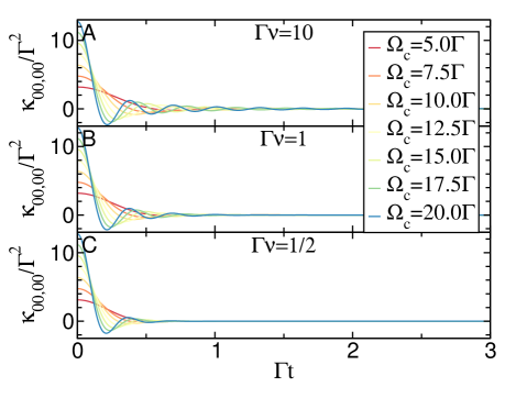
Figure 1: An element of the memory kernel $\kappa$ of the fully symmetric, resonant level model at a range of band parameters. Due to the symmetry, the results shown here are independent of both temperature and voltage. Panel A through C show the effect of softening the band edge by varying $\nu$, while within each separate panel the effect of varying the bandwidth (which is approximately twice the cutoff frequency $\Omega_{C}$) is illustrated.

The physics of the resonant level model are generally well known, yet the literature has seen little exploration of the properties of the memory kernel in this model, and of course none of the current memory kernel which has been introduced here. We therefore present some results below which we expect to be of interest to the field, as they provide insight into those aspects of the problem which do not rely on interaction. In order to restrict the parameter space explored, we will discuss the symmetric case in which $\varepsilon=0$ with a bias voltage applied symmetrically such that $V=2\mu_{L}=-2\mu_{R}$ (from here on we set $\hbar=e=1$). The lead coupling densities are taken to be $\Gamma_{L,R}\left(\omega\right)=\frac{1}{\left(1+e^{\nu\left(\omega-\Omega_{C}\right)}\right)\left(1+e^{\nu\left(-\omega-\Omega_{C}\right)}\right)}$. We will limit our attention only to the diagonal elements of the reduced density matrix and the corresponding element of the memory kernel; these elements are completely decoupled from the off-diagonal coherences, as discussed above, and therefore no approximation ensues from this.

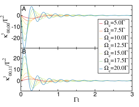
Figure 2: The two nonzero elements of $\kappa_{\iota}$ for the left current are shown in panels A and B, with $\Gamma\nu=10$, $\Gamma\beta=1$ and $V=4\Gamma$. In each panel, the time dependence of the $\kappa_{\iota}$ element is shown at a range of bandwidths.

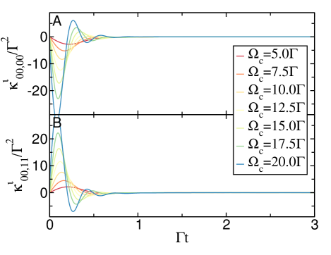
Figure 3: The two nonzero elements of $\kappa_{\iota}$ for the left current are shown in panels A and B, with $\Gamma\nu=0.5$, $\Gamma\beta=1$ and $V=4\Gamma$. In each panel, the time dependence of the $\kappa_{\iota}$ element is shown at a range of bandwidths.

All the results presented in this section are exact and have been calculated by a direct solution of the full equation of motion of the complete density matrix, a technique which relies on the quadratic form of the Hamiltonian and is therefore applicable only to the noninteracting case. In general, making similar progress for interacting systems requires a numerical solver of one type or another.Mühlbacher and Rabani (2008); Weiss et al. (2008); Werner et al. (2009); Wang and Thoss (2009b); Segal et al. (2010)

We begin with a discussion of the behavior of the memory kernel. The symmetrical parameters we have chosen are of particular interest because in the absence of interaction both $\sigma\left(t\right)$ and $\kappa\left(t\right)$ are completely independent of both the temperature and voltage. In addition, all nonzero matrix elements of $\kappa$ are all identical to within a sign ($\kappa_{00,00}=\kappa_{11,11}=-\kappa_{11,00}=-\kappa_{00,11}$). In Fig. 1 we therefore explore the dependence of one arbitrarily chosen element of $\kappa$ on a range of band parameters: cutoff energies $\Omega_{C}$ (the bandwidth is $\sim 2\Omega_{C}$) and band cutoff widths $\frac{1}{\nu}$. In each panel we go from a small bandwidth (red) to a large one (blue) at a set cutoff width, with the sharpest cutoff shown in panel A, an intermediate value in B and the smoothest in C.

The effect of the the two parameters describing our chosen band shape on the memory kernel can be understood quite well by considering the trends shown in the plot: as $\nu$ decreases, reflections are softened by the gradual slope at the band edge and the memory kernel decays more quickly. On the other hand, increasing the bandwidth induces oscillations at a frequency $\omega\approx\Omega_{C}$, but also increases the proportional weight of the short-time part of the memory kernel. Eventually, if we were to approach the wide band limit, the memory would approach the form of a delta function and a Markovian description of the dynamics would become exact.

The current memory kernel $\kappa_{\iota}$ is not as highly symmetric as $\kappa$, and depends to some extent on all the parameters of the problem. There are two distinct (though similar) elements in $\kappa_{\iota}$ at nonzero voltage, and these are plotted for the left current with $\Gamma\nu=10$ in panels A and B of Fig 2. The figure illustrates the dependence of $\kappa_{\iota}$ on the bandwidth, which exhibits the same properties observed in $\kappa$. This is also true of its $\nu$ dependence: to exemplify this, Fig 3 displays the same data for $\Gamma\nu=0.5$, where $\kappa_{\iota}$ decays more quickly and smoothly. Interestingly, the timescale over which $\kappa_{\iota}$ decays to zero does not appear to differ markedly from the corresponding timescale for $\kappa$ at similar parameters; this suggests that the cutoff approximation remains as useful for the current as it is for impurity observables.

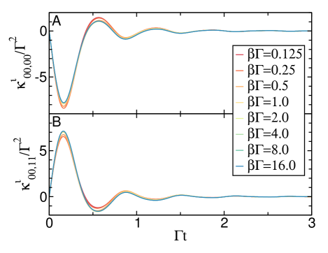
Figure 4: The two nonzero elements of $\kappa_{\iota}$ are shown in panels A and B, with $\Gamma\nu=10$, $\Omega_{c}=10\Gamma$ and $V=4\Gamma$. In each panel, the time dependence of the $\kappa_{\iota}$ element is shown at a range of inverse temperatures $\beta$.

The effect of temperature on $\kappa_{\iota}$ depends greatly on the choice of other parameters. At the parameters we have chosen for Fig. 4 the asymmetry between the two $\kappa_{\iota}$ elements is increased somewhat when the temperature is lowered, corresponding to an increase in the current (not shown). One would expect a rather different effect when, for instance, things are set up in such a way that thermal enhancement of the current occurs. Unlike $\kappa$, $\kappa_{\iota}$ depends on temperature even in the fully symmetric and noninteracting case is interesting, and expresses the fact that this quantity is connected to bath observables as well as to those in the impurity subspace.

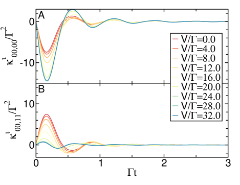
Figure 5: The two nonzero elements of $\kappa_{\iota}$ are shown in panels A and B, with $\Gamma\nu=10$, $\Omega_{c}=10\Gamma$ and $\Gamma\beta=1$. In each panel, the time dependence of the $\kappa_{\iota}$ element is shown at a range of bias voltages $V$.

Fig. 5 shows how voltage affects the current memory kernel: at zero voltage the two elements of $\kappa_{\iota}$ are identical up to a sign, and the application of a voltage increases the diagonal element while suppressing the off-diagonal terms. Additionally, an increase in the oscillation frequency is observed for $\kappa_{00,11}$, but no such clear trend exists for the oscillation frequency in $\kappa_{00,00}$. As $V$ passes the bandwidth ($\sim 20\Gamma$ here), the left lead becomes entirely occupied and the right entirely empty, and further increasing the voltage ceases to have any effect on the current memory kernel, just as occurs in the case of the current itself (not shown).

To show that the generalized NZME formalism introduced in this work indeed reproduces the correct results for the current as a function of time, Fig. 6 presents a comparison between the current obtained directly (lighter solid lines) and by way of Eq. (29) (darker dashed lines). Pairs of lines describing the two different ways of obtaining currents at identical parameters overlap to within numerical errors, expressing the equivalence between the two methods when convergence in the cutoff time has been attained and the correctness of the approach at the $t_{c}\rightarrow\infty$ limit.

Finally, while the NZME memory kernel technique and the cutoff approximation have been shown to be efficient for $\sigma$ in a variety of interacting and noninteracting cases,Cohen and Rabani (2011); Cohen et al. (2013); Wilner et al. meaning that results at long times $t\gg t_{c}$ converge at a finite $t_{c}$, no such calculations have previously been carried out for the generalized technique. This entails a convergence analysis of the type exemplified graphically in Fig. 7. In essence, the cutoff time $t_{c}$ must be increased until the desired accuracy is reached. In the example shown in Fig. 7, convergence is achieved quickly and even short-time oscillations beyond the range of $t_{c}$ are predicted with some accuracy (as can be seen from the extension of the oscillatory ridges beyond the boundary of the transparent $t=t_{c}$ plane). As an alternative (if partial) representation of this idea, in Fig. 8 several plane cuts through this function are shown, but this time at $\Gamma\nu=0.5$; both the current and its time derivative are displayed. The rapid convergence visible in either representation illustrates that the idea of the reduced dynamics technique and the cutoff approximation remains useful in practice even for the current, despite it being a non-system operator not accessible within the confines of the standard NZME formalism.

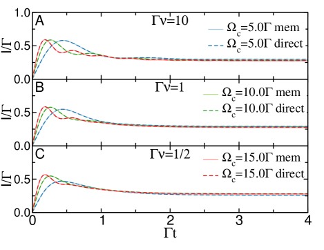
Figure 6: The left current is shown as a function of the physical time $t$ at a variety of band parameters. Dashed lines in dark colors correspond to exact results calculated directly. Each such line is paired with a solid line in a brighter color at the same parameters showing converged results obtained from tracing over the $\iota$ operator obtained from solving the generalized NZME Eq. (29). In all cases we have set $\Gamma\beta=1$ and $V=4\Gamma$.

VII Summary and conclusions

We have reviewed the process of implementing reduced dynamics techniques by way of the NZME and the memory cutoff approximation, which have recently been introduced with great success into several numerically exact nonequilibrium impurity solvers. The procedure of deriving a memory kernel scheme for a general impurity model and obtaining calculable expressions in terms of standard second-quantization operators was outlined, and the example of the noninteracting resonant level model was worked out in full detail. For this noninteracting case, some illustrative examples of the physical properties of the memory kernel were discussed.

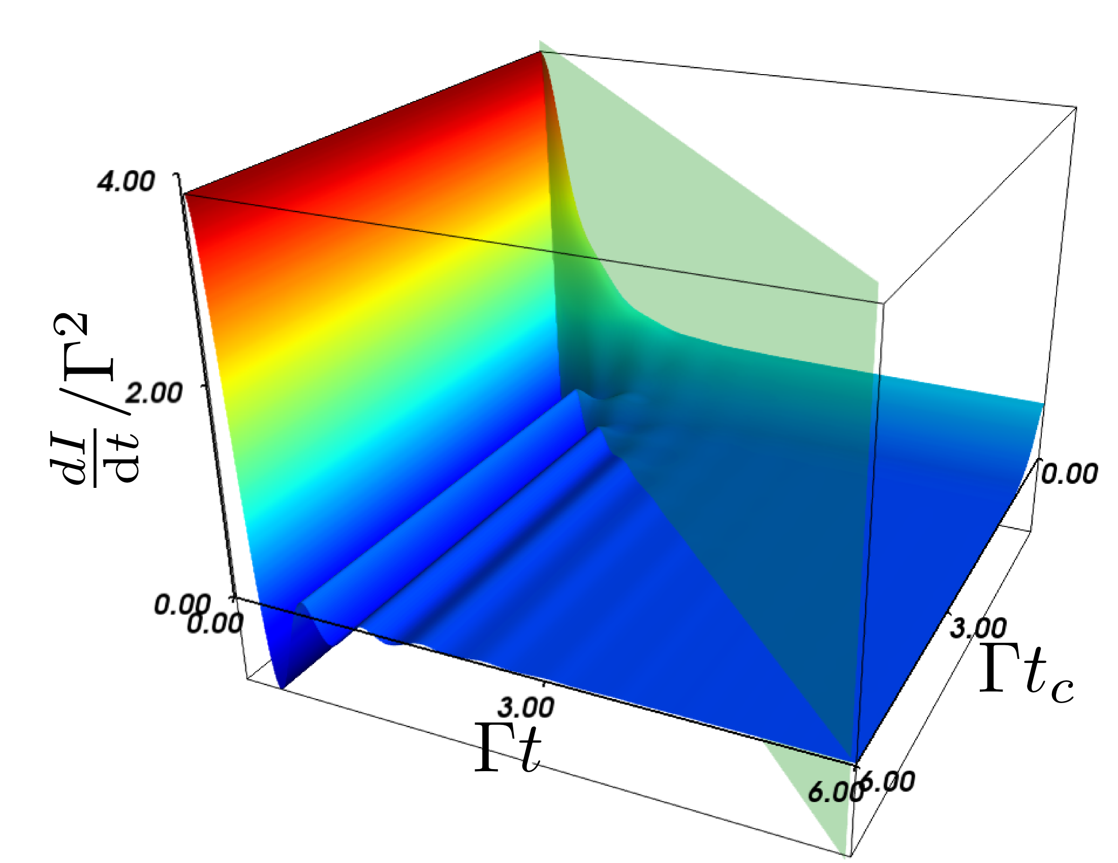
Figure 7: The time derivative of the left current in the cutoff approximation is shown as a function of both physical time $t$ and the cutoff time $t_{c}$. The transparent plane marks $t=t_{c}$, and for $t<t_{c}$ (to the left of the plane) the results are exact. To converge the results for the current within some numerical accuracy, one must increase $t_{c}$ until $\frac{\mathrm{dI\left(t\right)}}{\mathrm{d}t}$ ceases to vary within that accuracy. Parameters are $\Gamma\nu=10$, $\Omega_{c}=10\Gamma$, $\Gamma\beta=1$ and $V=4\Gamma$.

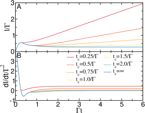
Figure 8: The left current (top) and its time derivative (bottom) are shown as a function of the physical time $t$ at $\Gamma\nu=0.5$, $\Omega_{c}=10\Gamma$, $\Gamma\beta=1$ and $V=4\Gamma$, for a range of cutoff times $t_{c}$. The final line, labeled $t_{c}=\infty$, shows the exact result for comparison.

An important limitation of the reduced dynamics techniques so far has been the lack of access to none-impurity observables, such as the electronic current in the resonant level model, the Anderson impurity model, and the Holstein model. A generalization of the NZME formalism which allows access to general operators was therefore introduced here, and the implementation of this formalism was carried through for the example of the current in the non-interacting limit. This led to the definition and evaluation of a current memory kernel $\kappa_{\iota}$, which was subsequently explored for its dependence on time, bandwidth, voltage and temperature. The validity of the cutoff approximation for the current memory kernel was then verified and discussed.

Looking forward, we expect the ideas expounded upon here to have several major implications: first, we hope to see them become a standard part of the toolbox of high quality time domain numerical simulations of impurity models, and extended to a variety of models and methods; in this context the memory technique should be viewed not as competing with existing direct solvers, but as a supplemental tool which allows efficient extension of any general short-time solver to long timescales, in situations where the memory timescale is short. Second, since access to current enables access to Green’s functions, the benefits offered by memory techniques are expected to be applicable to interacting lattice simulations as well, by way of mapping schemes such as dynamical mean field theory and its various extensions. Finally, we believe the memory kernel framework is a fertile ground for defining new approximation schemes more general than the cutoff approximation, and in this context it will be particularly interesting to understand the long-time behavior of the memory kernel in interacting cases and its behavior in larger impurity models.