Abstract

Effects of CP-violating phases in active-sterile solar neutrino oscillations are discussed in a general scheme of 3+$N_{s}$ mixing, without any constraint on the mixing between the three active and the $N_{s}$ sterile neutrinos, assuming only a realistic hierarchy of neutrino mass-squared differences. A generalized Parke formula describing the neutrino oscillation probabilities inside the Sun is calculated. The validity of the analytical calculation and the probability variation due to the unknown CP-violating phases are illustrated with a numerical calculation of the evolution equation in the case of 3+1 neutrino mixing.

PACS numbers: 14.60.St, 13.35.Hb, 14.60.Pq, 26.65.+t

1 Introduction

Despite the success of standard three-neutrino oscillations [1] in explaining the results of solar (SOL), atmospheric (ATM), reactor and accelerator neutrino experiments with two distinct mass-squared differences (i.e., $\Delta{m}^{2}_{\mathrm{SOL}}$ and $\Delta{m}^{2}_{\mathrm{ATM}}$) and three non-zero mixing angles (i.e., $\theta_{12}$, $\theta_{23}$ and $\theta_{13}$), some anomalies in short baseline (SBL) neutrino oscillation experiments (e.g., LSND [2], MiniBooNE [3], the Reactor anomaly [4] and Gallium anomaly [5]) indicate the existence of oscillations with much shorter baselines. This would imply the existence of extra mass-squared differences (i.e., $\Delta{m}^{2}_{\mathrm{SBL}}$) with the hierarchy

$$\Delta{m}^{2}_{\mathrm{SOL}}\ll\Delta{m}^{2}_{\mathrm{ATM}}\ll\Delta{m}^{2}_{\mathrm{SBL}}\quad,$$ (1)

and therefore the mixing of three active neutrinos with extra sterile neutrino states [6, 7, 8]. Furthermore, the analysis [9, 10] of cosmic microwave background and large scale structure data may hint at the existence of additional radiation in the Universe, with sterile neutrinos being one of the plausible candidates. One extra sterile neutrino is also allowed by recent analyses of Big Bang Nucleosynthesis [11]. Therefore, we should be open-minded on the existence of sterile neutrinos and it might be instructive to study the effects of the light sterile neutrino hypothesis in solar neutrino [12, 13, 14] and atmospheric neutrino [15] oscillation experiments or in non-oscillation processes including beta decay [16] and neutrinoless double-beta decay [17].

Solar neutrinos produced in the core of the Sun can undergo matter-enhanced Mikheev-Smirnov-Wolfenstein (i.e., MSW [18, 19]) oscillations when they propagate inside the Sun. When a generic scheme with one or more sterile neutrinos is considered, some sub-leading effects including the effects of light sterile neutrinos [20], non-unitarity of the lepton mixing matrix (NU) [21] and non-standard interactions (NSI) [22] may contribute to the neutrino oscillation probabilities and modify the standard MSW picture in the three-neutrino mixing scheme. Therefore, it is possible to constrain or measure these high-order effects with future precision solar neutrino experiments.

In an earlier work [12] by two of the present authors, we proposed a general method to calculate the matter effects of solar neutrino oscillations with an arbitrary number of sterile neutrinos, without any constraint on the magnitudes of the active-sterile mixing. However, the oscillation probabilities derived in Ref. [12] are only valid for a real neutrino mixing matrix because of an incorrect treatment of the CP-violating phases. As will be explained in Section 3, in Ref. [12] the effects of the CP-violating phases have been removed with an inappropriate phase-transformation.

In this work, we study the evolution of the neutrino flavor amplitudes inside the Sun by taking into account the roles of the CP-violating phases of the neutrino mixing matrix. We calculate the generalized Parke formula describing the electron neutrino survival probability and the electron-to-sterile neutrino transition probability. Furthermore, we validate our analytical calculations through a numerical solution of the neutrino evolution equation in the case of four-neutrino mixing and we illustrate numerically the effects on the survival and transition probabilities of the three CP-violating phases.

This paper is organized as follows. We review the general framework of neutrino flavor evolution in Sec. 2 and we present the analytical expressions for the neutrino oscillation probabilities in Sec. 3. In Sec. 4 a numerical validation of the analytical results and an illustration of the effects of the CP-violating phases is presented in the simplest case of four-neutrino mixing. Finally, we conclude in Sec. 5. At the end of the paper there are three appendices on the analytical derivation of the non-adiabatic crossing probability, on the explicit parametrization of the mixing matrix and on the density matrix method.

2 General Framework

Following the notation of Ref. [12], in this Section we shall give a brief review on the general framework of neutrino flavor evolution with three active and $N_{s}$ sterile neutrinos. The flavor eigenstates of active neutrinos and sterile neutrinos can be written as

$$\left|{\nu_{\alpha}}\right\rangle=\sum^{N}_{i=1}U^{*}_{\alpha i}\left|{\nu_{i}}\right\rangle\;,$$ (2)

where $N=3+N_{s}$, $\alpha$ runs over $e$, $\mu$ and $\tau$ for three active neutrinos and $s_{1},\ldots,s_{N_{s}}$ for $N_{s}$ sterile neutrinos, $\nu_{i}$ is one of the $N$ mass eigenstates with mass $m_{i}$, and $U_{\alpha i}$ stands for an element of the $(3+N_{s})\times(3+N_{s})$ neutrino mixing matrix. In the general case, solar neutrinos are described by the state

$$|\nu(x)\rangle=\sum_{\alpha=e,\mu,\tau,s_{1},\ldots,s_{N_{s}}}\psi_{\alpha}(x)|\nu_{\alpha}\rangle\quad,$$ (3)

where $x$ is the distance from the production point during the propagation with the initial condition $\psi_{\alpha}(0)=\delta_{\alpha e}$ and the normalization $\sum_{\alpha}|\psi_{\alpha}(x)|^{2}=1$. The Mikheev-Smirnov-Wolfenstein (MSW) equation[18, 19] describing the evolution of the flavor transition amplitudes $\psi_{\alpha}(x)$ is given by (see Ref. [23])

$$i\frac{\mathrm{d}}{\mathrm{d}x}\Psi=\mathcal{H}_{\rm F}\Psi=\left(U\mathcal{M}U^{\dagger}+\mathcal{V}\right)\Psi\quad,$$ (4)

with

$$\Psi=\hbox{} \hbox{}\left(\psi_{e},\psi_{\mu},\psi_{\tau},\psi_{s_{1}},\ldots,\psi_{s_{N_{s}}}\right)^{T}\quad,$$ (5)

$$\mathcal{M}=\hbox{} \hbox{}\mathrm{diag}\!\left(0,\frac{\Delta{m}^{2}_{21}}{2E},\frac{\Delta{m}^{2}_{31}}{2E},\frac{\Delta{m}^{2}_{41}}{2E},\ldots,\frac{\Delta{m}^{2}_{N1}}{2E}\right)\quad,$$ (6)

$$\mathcal{V}=\hbox{} \hbox{}\mathrm{diag}\!\left(V_{\mathrm{CC}}+V_{\mathrm{NC}},V_{\mathrm{NC}},V_{\mathrm{NC}},0,\ldots,0\right)\quad,$$ (7)

where $E$ is the neutrino energy and $\Delta{m}^{2}_{kj}=m_{k}^{2}-m_{j}^{2}\,$. The charged-current and neutral-current matter potentials are defined as

$$V_{\mathrm{CC}}=\sqrt{2}G_{\mathrm{F}}N_{e}\simeq 7.63\times 10^{-14}\,\frac{N_{e}}{N_{\mathrm{A}}\,\mathrm{cm}^{-3}}\,\mathrm{eV}\quad,\qquad V_{\mathrm{NC}}=-\frac{1}{2}\sqrt{2}G_{\mathrm{F}}N_{n}\quad,$$ (8)

where $G_{\mathrm{F}}$ is the Fermi constant, $N_{e}$ is the electron number density, $N_{n}$ is the neutron number density, and $N_{\mathrm{A}}$ is the Avogadro’s number. By using the definition of electron fraction $Y_{e}=N_{e}/(N_{e}+N_{n})$, we have

$$N_{e}=\frac{\rho}{\mathrm{g}}\,N_{\mathrm{A}}Y_{e}\quad,\qquad N_{n}=\frac{\rho}{\mathrm{g}}\,N_{\mathrm{A}}\left(1-Y_{e}\right)\quad,$$ (9)

in an electro-neutral medium, with $\rho$ being the mass density. Thus, we have the following relation between the two matter potentials:

$$V_{\mathrm{NC}}=R_{\mathrm{NC}}V_{\mathrm{CC}}\quad,\quad\mathrm{with}\quad R_{\mathrm{NC}}=-\frac{1-Y_{e}}{2Y_{e}}\quad.$$ (10)

Next, we can introduce the vacuum mass basis as

$$\Psi^{\mathrm{V}}=\left(\psi^{\mathrm{V}}_{1},\ldots,\psi^{\mathrm{V}}_{N}\right)^{T}=U^{\dagger}\Psi\quad,$$ (11)

which satisfies the following evolution equation

$$i\frac{\mathrm{d}}{\mathrm{d}x}\Psi^{\mathrm{V}}=\left(\mathcal{M}+U^{\dagger}\mathcal{V}U\right)\Psi^{\mathrm{V}}\quad.$$ (12)

Then we can decouple the flavor transitions generated by $\Delta{m}^{2}_{21}$ from those generated by the larger mass-squared differences, according to the following hierarchy

$$V_{\mathrm{CC}}\sim|V_{\mathrm{NC}}|\sim\frac{\Delta{m}^{2}_{21}}{2E}\ll\frac{|\Delta{m}^{2}_{k1}|}{2E}\quad\mathrm{for}\quad k\geq 3\quad,$$ (13)

for the solar matter density. Therefore, the N-component evolution equation Eq. (12) can be truncated to

$$i\frac{\mathrm{d}}{\mathrm{d}x}\begin{pmatrix}\psi^{\mathrm{V}}_{1}\\ \psi^{\mathrm{V}}_{2}\end{pmatrix} =\begin{pmatrix}\sum_{\alpha}|U_{\alpha 1}|^{2}\mathcal{V}_{\alpha}&\sum_{\alpha}U_{\alpha 1}^{*}U_{\alpha 2}\mathcal{V}_{\alpha}\\ \sum_{\alpha}U_{\alpha 2}^{*}U_{\alpha 1}\mathcal{V}_{\alpha}&\Delta m^{2}_{21}/(2E)+\sum_{\alpha}|U_{\alpha 2}|^{2}\mathcal{V}_{\alpha}\end{pmatrix}\begin{pmatrix}\psi^{\mathrm{V}}_{1}\\ \psi^{\mathrm{V}}_{2}\end{pmatrix}\quad,$$ (14)

and

$$\psi^{\mathrm{V}}_{k}(x) \simeq\psi^{\mathrm{V}}_{k}(0)\,\exp\!\left(-i\,\frac{\Delta{m}^{2}_{k1}x}{2E}\right)\quad,\quad\mathrm{for}\quad k\geq 3\quad.$$ (15)

By subtracting a diagonal term

$$\frac{\Delta{m}^{2}_{21}}{4E}+\frac{1}{2}\sum_{\alpha}\left(|U_{\alpha 1}|^{2}+|U_{\alpha 2}|^{2}\right)\mathcal{V}_{\alpha}\quad,$$ (16)

which generates an irrelevant common phase, the evolution equation in Eq. (14) can be written as

$$i\frac{\mathrm{d}}{\mathrm{d}x}\Psi^{\mathrm{V}}_{2} =\mathcal{H}^{\mathrm{V}}_{2}\Psi^{\mathrm{V}}_{2}\quad,$$ (17)

with $\Psi^{\mathrm{V}}_{2}=(\psi^{\mathrm{V}}_{1},\psi^{\mathrm{V}}_{2})^{\rm T}$ and

$$\mathcal{H}^{\mathrm{V}}_{2}=\begin{pmatrix}-\delta+V\cos 2\xi&V\sin 2\xi e^{i\varphi}\\ V\sin 2\xi e^{-i\varphi}&\delta-V\cos 2\xi\end{pmatrix}\quad,$$ (18)

where the variables $\delta$, $V$ and $\xi$ are defined as

$$\delta =\frac{\Delta m^{2}_{12}}{4E}\quad,$$ (19)

$$V\cos 2\xi =\sum_{\alpha}\left(|U_{\alpha 1}|^{2}-|U_{\alpha 2}|^{2}\right)\mathcal{V}_{\alpha}=\frac{1}{2}V_{\mathrm{CC}}X\quad,$$ (20)

$$V\sin 2\xi e^{i\varphi} =\sum_{\alpha}U_{\alpha 1}^{*}U_{\alpha 2}\mathcal{V}_{\alpha}=\frac{1}{2}V_{\mathrm{CC}}Y=\frac{1}{2}V_{\mathrm{CC}}|Y|e^{i\varphi}\quad,$$ (21)

with

$$X =|U_{e1}|^{2}-|U_{e2}|^{2}+R_{\mathrm{NC}}\sum_{\alpha=e,\mu,\tau}\left(|U_{\alpha 1}|^{2}-|U_{\alpha 2}|^{2}\right){}$$

$$=|U_{e1}|^{2}-|U_{e2}|^{2}-R_{\mathrm{NC}}\sum_{i=1}^{N_{s}}\left(|U_{s_{i}1}|^{2}-|U_{s_{i}2}|^{2}\right)\quad,$$ (22)

$$Y =2\left(U_{e1}^{*}U_{e2}+R_{\mathrm{NC}}\sum_{\alpha=e,\mu,\tau}U_{\alpha 1}^{*}U_{\alpha 2}\right){}$$

$$=2\left(U_{e1}^{*}U_{e2}-R_{\mathrm{NC}}\sum_{i=1}^{N_{s}}U_{s_{i}1}^{*}U_{s_{i}2}\right)\quad.$$ (23)

Therefore, we can obtain the full expressions for $\varphi$, $\xi$ and $V$ as

$$\varphi =\arg(Y)\quad,$$ (24)

$$\tan 2\xi =\frac{|Y|}{X}\quad,$$ (25)

$$V =\frac{1}{2}V_{\mathrm{CC}}\sqrt{X^{2}+|Y|^{2}}\quad.$$ (26)

To be more explicit, we can rewrite the Hamiltonian in Eq. (18) in a compact form:

$$\mathcal{H}^{\mathrm{V}}_{2}=\mathcal{M}_{2}+U^{\dagger}_{2}\mathcal{V}_{2}U_{2}\quad,$$ (27)

with $\mathcal{M}_{2}=\mathrm{diag}(-\delta,\delta)$, $\mathcal{V}_{2}=\mathrm{diag}(V,-V)$ and

$$U_{2} =W_{2}(\xi,\varphi)\equiv\begin{pmatrix}\cos\xi&\sin\xi e^{i\varphi}\\ -\sin\xi e^{-i\varphi}&\cos\xi\end{pmatrix}\quad,$$ (28)

where $W_{2}(\xi,\varphi)$ is the complex rotation matrix which can be generated by a real rotation matrix $R_{2}(\xi)$ and a diagonal phase matrix $D_{2}(\varphi)$ (see Ref. [23]),

$$W_{2}(\xi,\varphi) =D^{\dagger}_{2}(\varphi)R_{2}(\xi)D_{2}(\varphi)\quad,$$ (29)

$$R_{2}(\xi) \equiv\begin{pmatrix}\cos\xi&\sin\xi\\ -\sin\xi&\cos\xi\end{pmatrix}\quad,$$ (30)

$$D_{2}(\varphi) \equiv\mathrm{diag}(1,e^{i\varphi})\quad.$$ (31)

Using the definition of these effective parameters, we have obtained an evolution equation analogous to that in the two-neutrino mixing scheme. But one should keep in mind that the effective mixing angle $\xi$ and phase $\varphi$ are not simple mixing parameters given by a specific parametrization but medium-dependent parameters which are constant only when the electron fraction $Y_{e}$ remains unchanged along the neutrino propagation path.

To solve the evolution equation in Eq. (17), we can first diagonalize the Hamiltonian in Eq. (27) with a complex rotation

$$\Psi^{\mathrm{V}}_{2} =W_{2}(\omega,\varphi)\Psi^{\mathrm{M}}_{2}\quad,$$ (32)

where

$$\tan 2\omega =\frac{V\sin 2\xi}{\delta-V\cos 2\xi}\quad,$$ (33)

$\varphi$ is the complex phase defined in Eq. (24), and $\Psi^{\mathrm{M}}_{2}$ is the amplitude vector in the effective mass basis in matter. Then the evolution equation becomes

$$i\frac{\mathrm{d}}{\mathrm{d}x}\Psi^{\mathrm{M}}_{2} =\mathcal{H}^{\mathrm{M}}_{2}\Psi^{\mathrm{M}}_{2}\quad,$$ (34)

where the Hamiltonian can be decomposed into the adiabatic (ad) and non-adiabatic (na) parts,

$$\mathcal{H}^{\mathrm{M}}_{2} =\mathcal{H}^{\mathrm{M}}_{\mathrm{ad}}+\mathcal{H}^{\mathrm{M}}_{\mathrm{na}}{}$$

$$\equiv\begin{pmatrix}-\delta_{\mathrm{M}}&0\\ 0&\delta_{\mathrm{M}}\end{pmatrix}+\begin{pmatrix}-\dot{\varphi}\sin^{2}\omega&(\frac{1}{2}\dot{\varphi}\sin 2\omega-i\dot{\omega})e^{i\varphi}\\ (\frac{1}{2}\dot{\varphi}\sin 2\omega+i\dot{\omega})e^{-i\varphi}&\dot{\varphi}\sin^{2}\omega\end{pmatrix}\quad,$$ (35)

with

$$\delta_{\mathrm{M}} =\sqrt{(\delta-V\cos 2\xi)^{2}+(V\sin 2\xi)^{2}}{}$$

$$=\sqrt{(V-\delta\cos 2\xi)^{2}+(\delta\sin 2\xi)^{2}}\quad,$$ (36)

$$\dot{\varphi}\equiv\frac{\mathrm{d}\varphi}{\mathrm{d}x}\quad,\quad\dot{\omega}\equiv\frac{\mathrm{d}\omega}{\mathrm{d}x}\quad.$$ (37)

Finally, we can arrive at a formal solution of Eq. (34),

$$\left\{\begin{array}[]{ll}\overline{|\psi^{\mathrm{M}}_{1}(x_{d})|^{2}}&=|\psi^{\mathrm{M}}_{1}(0)|^{2}\left(1-P_{12}\right)+|\psi^{\mathrm{M}}_{2}(0)|^{2}P_{12}\\ \overline{|\psi^{\mathrm{M}}_{2}(x_{d})|^{2}}&=|\psi^{\mathrm{M}}_{1}(0)|^{2}P_{12}+|\psi^{\mathrm{M}}_{2}(0)|^{2}\left(1-P_{12}\right)\end{array}\right.\quad\,,$$ (40)

for the averaged amplitudes of solar neutrino evolution, where $x_{d}$ is the coordinate of the detector on the Earth, $P_{12}$ is the level-crossing probability between two effective mass eigenstates $\psi^{\mathrm{M}}_{1}$, $\psi^{\mathrm{M}}_{2}$ during their propagation inside the Sun. By definition, $P_{12}$ is zero when the off-diagonal terms in Eq. (35) are vanishing, which is defined as the adiabatic approximation.

Before finishing this Section, we want to point out that, as an improvement to the results in Ref.[12], in this paper we consider the general case in which the effective phase $\varphi$ cannot be absorbed by a simple rephasing transformation when the electron fraction $Y_{e}$ is not constant along the neutrino path. In this case, the CP-violating phases in the mixing matrix may influence the neutrino flavor evolution inside the Sun through the effective phase $\varphi$, which is the complex argument of $Y$ Eq. (23). Moreover, since also the module of $Y$ depends on the CP-violating phases in $U_{\alpha 1}$ and $U_{\alpha 2}$, these phases can affect also on the behavior of $\xi$, $V$ and $\omega$. In the next Section we derive the analytic expression for the average oscillation probabilities of solar neutrinos taking into account the effects of the CP-violating phases in the mixing matrix.

3 Generalized Parke Formula

In this Section, we derive the neutrino oscillation probabilities based on the framework presented in the previous Section. Due to the energy resolution of the detector and the uncertainty of the production region, the interference terms between the massive neutrinos are not measurable [25]. As a result, we obtain the averaged oscillation probabilities

$$\overline{P}^{\mathrm{S}}_{\nu_{e}\to\nu_{\beta}}= \overline{|\psi_{\beta}(x_{d})|^{2}}=\overline{\left|\sum_{k=1}^{N}U_{\beta k}\psi^{\mathrm{V}}_{k}(x_{d})\right|^{2}}{}$$

$$= \sum_{k=1}^{N}|U_{\beta k}|^{2}\overline{|\psi^{\mathrm{V}}_{k}(x_{d})|^{2}}{}$$

$$= \sum_{k=1}^{2}|U_{\beta k}|^{2}\overline{|\psi^{\mathrm{M}}_{k}(x_{d})|^{2}}+\sum_{k=3}^{N}|U_{\beta k}|^{2}|\psi^{\mathrm{V}}_{k}(0)|^{2}\quad,$$ (41)

where the matter effects in the detector are neglected. According to Eq. (15), $\psi^{\mathrm{V}}_{k}$ with ($k\geq 3$) is decoupled from other amplitudes inside the Sun and evolves independently. All we need is to solve the evolution equation in the truncated 1-2 sector, given in Eq. (17) in the vacuum basis or in Eq. (34) in the effective mass basis in matter. From the initial conditions for the flavor amplitudes $\psi_{\beta}(0)=\delta_{\beta e}$, one obtain that in the vacuum basis $\psi^{\mathrm{V}}_{k}(0)=U_{ek}^{*}$.

Writing $U_{\beta 1}$ and $U_{\beta 2}$ as

$$\left\{\begin{array}[]{ll}U_{\beta 1}&=\cos\theta_{\beta}\,\cos\chi_{\beta}\,e^{i\,\phi_{\beta 1}}\\ U_{\beta 2}&=\sin\theta_{\beta}\,\cos\chi_{\beta}\,e^{i\,\phi_{\beta 2}}\end{array}\right.\quad\text{with}\quad\cos^{2}\chi_{\beta}=|U_{\beta 1}|^{2}+|U_{\beta 2}|^{2}\quad,$$ (42)

the initial conditions in the effective mass basis in matter are

$$\left\{\begin{array}[]{ll}\psi^{\mathrm{M}}_{1}(0)&=\cos\chi_{e}(\cos\omega^{0}\cos\theta_{e}e^{-i\phi_{e1}}-\sin\omega^{0}\sin\theta_{e}e^{-i(\phi_{e2}-\varphi^{0})})\\ \psi^{\mathrm{M}}_{2}(0)&=\cos\chi_{e}(\sin\omega^{0}\cos\theta_{e}e^{-i(\varphi^{0}+\phi_{e1})}+\cos\omega^{0}\sin\theta_{e}e^{-i\phi_{e2}})\end{array}\right.\quad,$$ (45)

where $\omega^{0}$ and $\varphi^{0}$ are the rotation parameters [see the definition in Eq. (32)] between the vacuum mass basis and effective mass basis at the production point.

Using the relations in Eq. (40), we obtain the averaged solar neutrino oscillation probabilities

$$\overline{P}^{\mathrm{S}}_{\nu_{e}\to\nu_{\beta}} =\cos^{2}\chi_{e}\cos^{2}\chi_{\beta}\overline{P}^{\mathrm{(2\nu)}}_{\nu_{e}\to\nu_{\beta}}+\sum_{k=3}^{N}|U_{ek}|^{2}|U_{\beta k}|^{2}\quad,$$ (46)

with

$$\overline{P}^{\mathrm{(2\nu)}}_{\nu_{e}\to\nu_{\beta}} \equiv\frac{1}{2}+(\frac{1}{2}-P_{12})\cos 2\theta_{\beta}[\cos 2\theta_{e}\cos 2\omega^{0}-\cos\Phi^{0}\sin 2\theta_{e}\sin 2\omega^{0}]\quad,$$ (47)

where

$$\Phi^{0}=\phi_{e1}-\phi_{e2}+\varphi^{0}\,.$$ (48)

One can check that the survival probability reduces to the well-known Parke formula [26] in the limit of two-neutrino mixing, in which $\cos^{2}\chi_{e}=\cos^{2}\chi_{\beta}=\cos\Phi^{0}=1$ and $[\cos 2\theta_{e}\cos 2\omega^{0}-\cos\Phi^{0}\sin 2\theta_{e}\sin 2\omega^{0}]\to\cos 2\theta_{e}^{0}$, where $\theta_{e}^{0}=\theta_{e}+\omega^{0}$ is the effective mixing angle between the flavor basis and the effective mass basis in matter at the production point.

The oscillation probabilities reduce to the ones in Ref. [12] in the case of CP invariance, in which $\cos\Phi^{0}=1$. Note, however, that in the case of CP violation the expression (46) for the oscillation probabilities do not reduce to the corresponding Eq. (61) of Ref. [12] even if the electron fraction $Y_{e}$ is constant along the neutrino path. In this case, as explained in Ref. [12] one can eliminate the phase $\varphi$ by an appropriate rephasing of the mixing matrix. In fact, since the MSW evolution equation (4) is invariant under the phase transformation

$$U_{\alpha k}\to e^{i\varphi_{\alpha}}U_{\alpha k}e^{i\varphi_{k}}\,,$$ (49)

which transforms $\varphi\to\varphi+\varphi_{2}-\varphi_{1}$, one can eliminate $\varphi$ by choosing $\varphi_{1}-\varphi_{2}=\varphi$. However, in this case there is no remaining phase freedom to eliminate both $\phi_{e1}$ and $\phi_{e2}$, contrary to what has been incorrectly stated in Ref. [12]. Indeed, since $\phi_{e1}-\phi_{e2}+\varphi$ is invariant under the phase transformation (49) (as well as $X$ and $|Y|$, and hence $\overline{P}^{\mathrm{S}}_{\nu_{e}\to\nu_{\beta}}$), it is clear that it cannot be eliminated. Hence, the oscillation probabilities in Eq. (46) represents the improvement of the corresponding oscillation probabilities in Eq. (61) of Ref. [12] which takes into account in a proper way the effect of the CP-violating phases in the mixing matrix .

The CP-violating phases can contribute to the oscillation probabilities in several different aspects. It is obvious to identify $\cos\Phi^{0}$ as a term which gives a direct impact, but in practice $\cos\Phi^{0}$ is very close to unity for solar neutrinos, as shown in the next Section (see, for example, Fig. 7). However, there can be a significant phase dependence of the oscillation probabilities coming from $\omega^{0}$, which depends on the CP-violating phases through $X$ and $|Y|$ and through the modules of the mixing matrix elements in two different rows, which depend on the cosines of the CP-violating phases.

When counting the relevant number of CP-violating phases in solar neutrino oscillations, one should take into account that $\nu_{\mu}$ and $\nu_{\tau}$ are indistinguishable and all sterile neutrinos are indistinguishable. Therefore, if the mixing matrix is written as a product of complex rotations, the rotation in the $\nu_{\mu}$-$\nu_{\tau}$ sector and all the complex rotations among sterile neutrinos do not have any effect on the observables in solar neutrinos. These complex rotations can be eliminated from the evolution equation (12) by choosing a parameterization of the mixing matrix in which they occupy the left-most positions. Then, the remaining part of the mixing matrix can be written in terms of two complex rotations among active neutrinos and three complex rotations between the three active neutrinos and each sterile neutrino, with a total of $2+3N_{s}$ complex rotations. Of the corresponding phases, there are $2+N_{s}$ Majorana phases which can be factorized in a diagonal matrix on the right of the mixing matrix (see Section 6.7.3 of Ref. [23]) and have no effect on oscillations. Therefore, solar neutrino oscillations depend on $2N_{s}$ Dirac CP-violating phases.

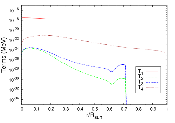
Figure 1: The magnitudes of four different terms in Eq. (35): $T_{1}=\delta_{\mathrm{M}}$, $T_{2}=|\dot{\varphi}\sin^{2}\omega|$, $T_{3}=|\frac{1}{2}\dot{\varphi}\sin 2\omega|$ and $T_{4}=|\dot{\omega}|$. The mixing parameters are set to M1 and P1 in Appendix B and the matter density distribution is taken from the BSB2005(OP) Standard Solar Model [30].

In conclusion of this Section, let us discuss the problem of calculation of the crossing probability $P_{12}$. In Appendix A we describe two different approximations which allow us to derive analytical expressions for $P_{12}$. The first method [12], described in Appendix A.1, can be applied when the electron fraction $Y_{e}$ is approximately constant along the neutrino propagation path. In this case, we can employ the similarity of the neutrino flavor evolution in Eq. (34) to that of two-neutrino mixing and obtain the crossing probability with the help of non-perturbative calculations [27]. The second method, described in Appendix A.2, can be applied when the non-adiabatic contribution in the Hamiltonian (35) is much smaller than the adiabatic one. In this case, one can use the general perturbation theory [28, 29] and calculate the effective crossing probability to include the non-adiabatic contribution along the whole path of neutrino propagation inside the Sun.

Both of the above approximations are quite good for the solar neutrino evolution inside the Sun. As shown in Fig. 1 of Ref. [12], the electron fraction $Y_{e}$ is almost constant in the radiative ($0.25\lesssim r\lesssim 0.7$) and convective ($r\gtrsim 0.7$) zones, with the only exception of the core region with $r\lesssim 0.25$. However, the effects of the variation of $Y_{e}$ in the core are negligible if the flavor transitions occur mainly in a resonance located in the radiative or convective zone. The numerical analysis in Ref. [12] validated this approximation. For the approximation of perturbative expansion, we show the magnitudes of different terms of Eq. (35) in Fig. 1, considering, as an example, the values of the mixing parameters M1 and P1 in Appendix B and using the matter density distribution in the BSB2005(OP) Standard Solar Model [30]. One can see that the order of magnitude of the non-adiabatic terms can only reach at most about $0.1\%$ of the adiabatic term, verifying the accuracy of the perturbative approximation. In practice, the numerical calculations of $P_{12}$ with the two methods are consistent and both show that $P_{12}$ is negligibly small. Therefore, in the numerical analysis discussed in the following Section we neglect the crossing probability $P_{12}$.

4 Numerical Discussion

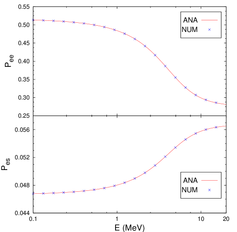
Figure 2: Energy spectra of the analytical and numerical evaluations of the solar neutrino electron survival (upper panel) and electron-to-sterile transition (lower panel) probabilities. All the oscillation parameters are set to M1 and P1 in Appendix B.

In this Section, we illustrate the validity of the neutrino oscillation probabilities in Eq. (46) and the effects of the CP-violating phases by using a numerical calculation of the neutrino evolution equation in the scheme of four-neutrino mixing. The explicit parametrization of the $4\times 4$ neutrino mixing matrix and the values of the oscillation parameters used in the discussion are presented in Appendix B.

As explained in Section 3, in the case $N_{s}=1$ the observable effects of solar neutrino oscillations depend on two Dirac CP-violating phases. In fact, we can write the mixing matrix as $U=W^{23}U^{\prime}$, where $W^{23}=W(\theta_{23},\eta_{23})$ is defined in Eq. (69) and $U^{\prime}$ is a proper product of the other rotations, which contains two Dirac CP-violating phases. Since $W^{23}$ drops out of the evolution equation (12), the oscillation probabilities are independent from $\eta_{23}$ (as well as from $\theta_{23}$). They depend only on the two Dirac CP-violating phases in $U^{\prime}$. However, in the following we will discuss the possibility to reveal the effects of the phases in a future scenario in which the absolute values $|U_{\alpha 4}|$ of the elements of the mixing matrix with $\alpha=e,\mu,\tau$ have been determined by precision short-baseline neutrino oscillation experiments. Hence, we adopt the parametrization in Appendix B in which $|U_{e4}|$, $|U_{\mu 4}|$ and $|U_{\tau 4}|$ are independent of the phases and determine the mixing angles $\theta_{14}$, $\theta_{24}$ and $\theta_{34}$ (there is no way to get such result with $U=W^{23}U^{\prime}$). Hence, although in the following we consider the three CP-violating phases in the parametrization in Appendix B, one should keep in mind that the oscillation probabilities depend only on two phases, which are complicated functions of the three CP-violating phases and of the mixing angles in the parametrization in Appendix B.

We employ the data of the matter density distribution in the BSB2005(OP) Standard Solar Model [30] and we consider, for simplicity, neutrinos produced at the solar center. To obtain the numerical evolution of solar neutrinos inside the Sun, we use the fourth-order Runge-Kutta method described in Numerical Recipes [34]. Since the unitarity condition is not automatically guaranteed in a straightforward application of the evolution equation in Eq. (17) and can be violated by the errors of the numerical computation, especially for the evolution in the crucial resonance region where the amplitudes oscillate rapidly, we employ the equivalent density matrix formalism (e.g., see Chapter 9 in Ref. [23]) in which the unitarity condition is fulfilled by definition. We refer to Appendix C for a brief introduction on the basics of the density matrix method.

In Fig. 2 we compare the analytical forms (ANA) of the electron neutrino survival probability $P_{ee}\equiv\overline{P}^{\mathrm{S}}_{\nu_{e}\to\nu_{e}}$ and the electron-to-sterile neutrino transition probability $P_{es}\equiv\overline{P}^{\mathrm{S}}_{\nu_{e}\to\nu_{s}}$ given by Eq. (46) with the corresponding numerical evaluations (NUM) of the neutrino flavor transitions. The upper and lower panels represent the electron survival and electron-to-sterile transition probabilities, respectively. We illustrate the comparisons with solid lines and cross points for the analytical and numerical oscillation probabilities, which show a perfect agreement between two different calculations of the evolution equation. Numerically, the accuracy of the analytical calculation is better than $10^{-5}$ and no systematic deviation appears.

Next, we want to illustrate the effects of the CP-violating phases in solar neutrino active-sterile oscillations. We can observe from Eq. (46) that the oscillation probabilities are only sensitive to the absolute values of the elements of the neutrino mixing matrix, except for the explicit contribution of the phases in $\cos\Phi^{0}$. However, as discussed in the last Section, the CP-violating phases determine also the contributions of the modules of the elements of the mixing matrix, since two distinct rows (i.e., the electron and sterile rows) are involved in the oscillation probabilities. In the specific parametrization of the neutrino mixing matrix presented in Appendix B, the modules of the matrix elements in the electron row are independent of the CP-violating phases, but those in other rows are phase-dependent. Therefore, the effects of the CP-violating phases in the electron neutrino survival probability arise only in the effective two-neutrino oscillation probability in Eq. (47) via the effective mixing parameters $\omega^{0}$ and $\Phi^{0}$. On the other hand, the CP-violating phases manifest themselves in the electron-to-sterile neutrino transition probability by the phase dependence in $\omega^{0}$, $\Phi^{0}$, $\theta_{s}$, $\chi_{s}$. Note that the constant term in Eq. (46) (i.e., $\sum_{k=3}^{4}|U_{ek}|^{2}|U_{sk}|^{2}$) depends on the variations of the CP-violating phases via $\chi_{s}$ in our specific parametrization.

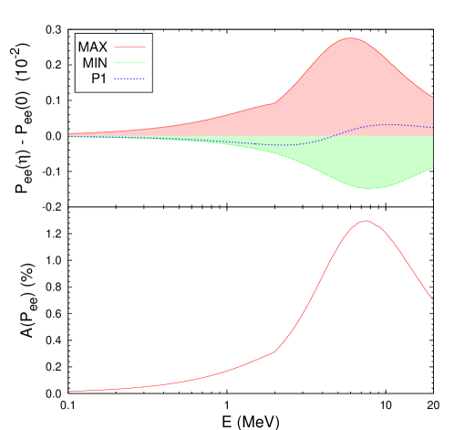
Figure 3: Energy spectra of ${\rm P}_{ee}(\eta)-{\rm P}_{ee}(0)$ (upper panel) and $A({\rm P}_{ee})$ (lower panel) for the electron neutrino survival probability. The mass and mixing parameters are set to M1 in Appendix B and the three CP-violating phases are randomly scanned in the full parameter space. The short-dashed line in the upper panel corresponds to the set of phases P1 in Appendix B.

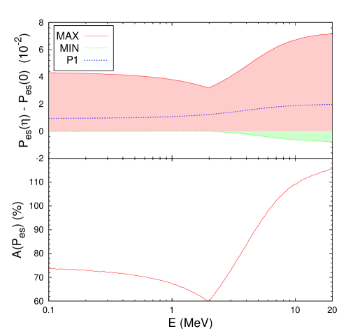
Figure 4: Same as Fig. 3, but for the electron-to-sterile neutrino transition probability.

Figure 5: Energy spectrum of $\cos 2\Theta^{0}_{e}$ in Eq. (51). The mass and mixing parameters are taken as M1 in Appendix B and the three CP-violating phases are randomly scanned in the full parameter space.

To show the variation of the oscillation probabilities for different values of the CP-violating phases, we can measure the possible size of the probability variation as the difference between the maximal (MAX) and minimal (MIN) values of the probabilities in the full parameter space of the three CP-violating phases. Therefore, we define the following asymmetries of the oscillation probabilities:

$$A(Q)=2\times\frac{{\rm MAX}[Q]-{\rm MIN}[Q]}{{\rm MAX}[Q]+{\rm MIN}[Q]}\,\quad,$$ (50)

where $Q$ could be either the survival or transition probabilities. Each asymmetry illustrate the possible variation of the corresponding probability depending on the unknown values of the CP-violating phases in a future scenario in which the absolute values $|U_{\alpha 4}|$ of the elements of the mixing matrix with $\alpha=e,\mu,\tau$ have been determined by precision short-baseline neutrino oscillation experiments [20]. In the following numerical discussion we consider, as a realistic example, the values M1 in Eq. (82) of the mixing angles, which determine the absolute values of the relevant elements of the mixing matrix through Eqs. (71)–(75).

In the lower panels of Figs. 3 and 4 we show the energy dependence of the asymmetries $A(P_{ee})$ and $A(P_{es})$. In the upper panels we show the possible range of variation of the probabilities $P_{ee}$ and $P_{es}$ for all possible values of the phases $\eta_{14}$, $\eta_{24}$, $\eta_{34}$, with respect to the case $\eta_{14}=\eta_{24}=\eta_{34}=0$. The shadowed regions with red and green colors are generated by scanning the full parameter space of three CP-violating phases. The two boundary curves stand for the maximal and minimal values of the differences (which correspond to the maximal and minimal values of the corresponding probability). These maximal and minimal values are used in calculating the corresponding asymmetry $A(P_{ee})$ or $A(P_{es})$ in the lower panels of Figs. 3 and 4. Note that the boundary curves may correspond to different values of the CP-violating phases for different energies.

In the upper panels of Figs. 3 and 4 we have also shown the curves corresponding to the values P1 in Eq. (84) of the CP-violating phases. We can observe that the variation induced by these values of the three CP-violating phases is less than $1.2\%$ for the electron survival probability and can be as large as $100\%$ for the electron-to-sterile transition probability. This is because the phase-independent contribution dominates in $P_{ee}$, whereas both the phase-independent and phase-dependent contributions are comparable in $P_{es}$ and both can induce significant variations in the transition probability. Notice that there is a kink and a sudden turn at about 2 MeV in the spectra of $A({\rm P}_{ee})$ and $A({\rm P}_{es})$, respectively, which correspond to the similar behaviour of the MAX boundary curves in the upper panels. This property can be understood with the help of Fig. 5, which shows the energy spectrum of the quantity

$$\cos 2\Theta_{e}^{0}\equiv\cos 2\theta_{e}\cos 2\omega^{0}-\cos\Phi^{0}\sin 2\theta_{e}\sin 2\omega^{0}$$ (51)

in Eq. (47) with randomly scanned CP-violating phases. Since $\cos 2\Theta^{0}_{e}$ changes sign at about 2 MeV, the values of the CP-violating phases which maximize the probability have a sudden jump, which generates a sudden change of the slope of the curve of maximal probability.

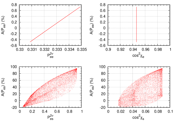
Figure 6: Scatter plots of the asymmetries $A({\rm P}_{ee})$ and $A({\rm P}_{es})$ with respect to the contributions of the first two mass eigenstates (${\rm P}^{2\nu}_{ee}$ or ${\rm P}^{2\nu}_{es}$) and those of all the other mass eigenstates ($\cos^{2}\chi_{e}$ or $\cos^{2}\chi_{s}$).

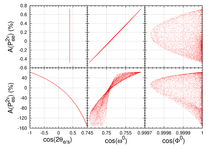
Figure 7: Scatter plots of the asymmetries $A({\rm P}^{2\nu}_{ee})$ and $A({\rm P}^{2\nu}_{es})$ versus $\cos 2\theta_{\rm e/s}$, $\cos\omega^{0}$ and $\cos\Phi^{0}$.

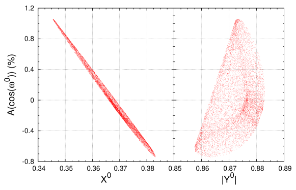
Figure 8: Scatter plots of the asymmetries $A(\cos\omega^{0})$ versus $X^{0}$ and $|Y^{0}|$.

Let us now discuss separately the different contributions to the probability variation. In Fig. 6 we show the scatter plots of $A(P_{ee})$ versus $\cos^{2}\chi_{e}$ and ${\rm P}^{2\nu}_{ee}$ and of $A(P_{es})$ versus $\cos^{2}\chi_{s}$ and ${\rm P}^{2\nu}_{es}$ obtained with a random generation of the three CP-violating phases in the entire parameter space. We considered a neutrino energy of 10 MeV and the mixing parameters M1 in Appendix B. Fig. 6 shows that the effects of the CP-violating phases show up only in the effective two-neutrino probability ${\rm P}^{2\nu}_{ee}$ for the survival probability $P_{ee}$, but emerge in both ${\rm P}^{2\nu}_{es}$ and the suppression factor $\cos^{2}\chi_{s}$ induced by the other neutrino states for the transition probability $P_{es}$. Moreover, we can further study separately the phase dependence of ${\rm P}^{2\nu}_{ee}$ and ${\rm P}^{2\nu}_{es}$ due to the phase dependence of $\cos^{2}\theta_{e/s}$, $\cos\omega^{0}$ and $\cos\Phi^{0}$, which is illustrated in the scatter plots in Fig. 7. In our parametrization of the mixing matrix, $\cos 2\theta_{e}$ is independent of the CP-violating phases, but $\cos 2\theta_{s}$ can reach almost all the possible values with the varying phase parameters. Therefore, the variation of the two-neutrino survival probability ${\rm P}^{2\nu}_{ee}$ is dominated by the changing of $\cos\omega^{0}$, but the variation of the two-neutrino transition probability ${\rm P}^{2\nu}_{es}$ comes from the phase dependence of $\cos 2\theta_{s}$ and $\cos\omega^{0}$. On the other hand, from the rightmost panels of Fig. 7, $\cos\Phi^{0}$ is very close to unity in both the survival and transition probabilities. This fact can be explained by considering Eq. (24), where the imaginary part of $Y$ is suppressed by both the small active-sterile mixing and the small neutral current contribution ($R_{\rm NC}\simeq-0.2$). Finally, the scatter plots in Fig. 8 show the correlations of the variations of $\cos\omega^{0}$ with those of $X^{0}$ and $|Y^{0}|$. One can see that the variation of $\cos\omega^{0}$ is mainly determined by $X^{0}$ rather than $|Y^{0}|$, because of the small phase dependence of $|Y|$.

In summary, we can conclude that the variation of the survival probability $P_{ee}$ due to the unknown CP-violating phases in the mixing matrix is determined mainly by the contribution of $\omega^{0}$, whereas the transition probability $P_{es}$ is sensitive to the CP-violating phases via $\chi_{s}$, $\theta_{s}$ and $\omega_{0}$, and the most significant contribution comes from $\theta_{s}$. We have also shown that the direct phase dependence of the probabilities through $\cos\Phi^{0}$ in Eq. (47) is negligible because $\cos\Phi^{0}$ is very close to one in the full parameter space.

5 Conclusion

In this work, we have calculated the analytical solution of the flavor evolution of solar neutrinos in a general scheme of 3+$N_{s}$ neutrino mixing, without any constraint on the mixing between the three active and the $N_{s}$ sterile neutrinos. We have improved the previous study in Ref. [12] by including the possible roles of the CP-violating phases in the mixing matrix and we have discussed the effects of these phases in active-sterile neutrino oscillations. We derived generalized Parke formulae which are suitable to be used in future precision measurements of solar neutrino oscillations.

In Section 4 we have presented a numerical discussion with a realistic example of the possible phase contribution to the oscillation probabilities in the case of 3+1 neutrino mixing. We validated the analytical formulae with a careful numerical solution of the evolution equation inside the Sun. We illustrated the effects of the CP-violating phases through an appropriate asymmetry of the oscillation probabilities. We have shown that, in our example, the variations induced by the three unknown CP-violating phases can reach the level of $1\%$ for the electron survival probability and may be as large as $100\%$ for the electron-to-sterile transition probability. This scenario will be realized when the absolute values of the elements of the mixing matrix $|U_{\alpha 4}|$ for $\alpha=e,\mu,\tau$ will be measured in precision short-baseline neutrino oscillation experiments. In this case, it might be possible to observe the effects of the CP-violating phases in future solar neutrino experiments.

Appendix A Analytical Derivation of $P_{12}$

In this Appendix, we present two methods for the approximate calculation of the crossing probability $P_{12}$: the constant $Y_{e}$ approximation and the approximation of perturbative expansion.

A.1 Constant $Y_{e}$ Approximation

Let us consider a case in which $Y_{e}$ is approximately constant inside the Sun. Then, $R_{\mathrm{NC}}$, $\xi$ and $\varphi$ remain approximately unchanged during the neutrino propagation. Therefore, we can introduce the tilded vacuum mass basis defined by

$$\tilde{\Psi}^{\mathrm{V}}_{2} =D_{2}(\varphi)\Psi^{\mathrm{V}}_{2}\quad,$$ (52)

to accommodate the phase $\varphi$ inside the amplitude vector ($D_{2}(\varphi)$ is defined in Eq. (31)). In the new basis, the evolution equation in Eq. (17) becomes

$$i\frac{\mathrm{d}}{\mathrm{d}x}\tilde{\Psi}^{\mathrm{V}}_{2} =\tilde{\mathcal{H}}^{\mathrm{V}}_{2}\tilde{\Psi}^{\mathrm{V}}_{2}\quad,$$ (53)

with $\tilde{\Psi}^{\mathrm{V}}_{2}=(\tilde{\psi}^{\rm V}_{1},\tilde{\psi}^{\rm V}_{2})^{\rm T}$ and

$$\tilde{\mathcal{H}}^{\mathrm{V}}_{2}=\begin{pmatrix}-\delta+V\cos 2\xi&V\sin 2\xi\\ V\sin 2\xi&\delta-V\cos 2\xi\end{pmatrix}\quad,$$ (54)

Meanwhile, we can decompose the Hamiltonian into the vacuum and matter parts as

$$\tilde{\mathcal{H}}^{\mathrm{V}}_{2}=\mathcal{M}_{2}+\tilde{U}_{2}^{\dagger}\mathcal{V}_{2}\tilde{U}_{2}\quad,$$ (55)

with $\tilde{U}_{2}=R_{2}(\xi)$ [defined in Eq. (30)].

As in the discussions in Ref. [12], we can further introduce the tilded effective interaction basis $\tilde{\Psi}^{\mathrm{I}}_{2}$ and the tilded effective mass basis $\tilde{\Psi}^{\mathrm{M}}_{2}$ in matter defined by

$$\tilde{\Psi}^{\mathrm{I}}_{2}=R_{2}(\xi)\tilde{\Psi}^{\mathrm{M}}_{2}\,,\quad\quad\tilde{\Psi}^{\mathrm{V}}_{2}=R_{2}(\omega)\tilde{\Psi}^{\mathrm{M}}_{2}\,.$$ (56)

In this way, we obtain evolution equations for $\tilde{\Psi}^{\mathrm{I}}_{2}$ and $\tilde{\Psi}^{\mathrm{M}}_{2}$ which have the same form as those without the CP-violating phases [12] if all the quantities with tildes are replaced by those without tildes. For instance, in the $\tilde{\Psi}^{\mathrm{M}}_{2}$ basis the evolution equation can be written as

$$i\frac{\mathrm{d}}{\mathrm{d}x}\tilde{\Psi}^{\mathrm{M}}_{2} =\begin{pmatrix}-\delta_{\mathrm{M}}&-i\dot{\omega}\\ i\dot{\omega}&\delta_{\mathrm{M}}\end{pmatrix}\tilde{\Psi}^{\mathrm{M}}_{2}\quad,$$ (57)

which is just the standard evolution equation of two-neutrino mixing in matter [23]. From the similarity we can define the adiabaticity parameter

$$\gamma=\frac{\delta_{\mathrm{M}}}{|\dot{\omega}|}=\frac{2\delta_{\mathrm{M}}^{\,3}}{V\delta\sin 2\xi|\mathrm{d}\ln N_{e}/\mathrm{d}x|}\quad,$$ (58)

and obtain the crossing probability $P_{12}$ as

$$P_{12}=\frac{\exp\left(-\frac{\pi}{2}\gamma_{\mathrm{R}}F\right)-\exp\left(-\frac{\pi}{2}\gamma_{\mathrm{R}}\frac{F}{\sin^{2}\xi}\right)}{1-\exp\left(-\frac{\pi}{2}\gamma_{\mathrm{R}}\frac{F}{\sin^{2}\xi}\right)}\,\theta\left(V_{0}-V_{\mathrm{R}}\right)\quad,$$ (59)

where $V_{\mathrm{R}}=\delta\cos 2\xi$ defines the resonance point and $\gamma_{\mathrm{R}}$ is the adiabaticity parameter at the resonance with

$$\gamma_{\mathrm{R}}=\frac{2\delta\sin^{2}2\xi}{\cos 2\xi\left|\mathrm{d}\ln N_{e}/\mathrm{d}x\right|_{\mathrm{R}}}\quad,$$ (60)

Finally, the $\theta$ function is used to reduce $P_{12}$ to zero when the potential at the production point is smaller than that at the resonance point. We use $F=1-\tan^{2}\xi$ for an exponential density profile, which is a good approximation for the solar neutrinos [27].

A.2 Perturbative Expansion

As discussed in Section 3, the non-adiabatic terms are much smaller that the adiabatic term and we can treat $\mathcal{H}^{\mathrm{M}}_{\mathrm{na}}$ in Eq. (35) as a perturbation term relative to $\mathcal{H}^{\mathrm{M}}_{\mathrm{ad}}$. Therefore, we can solve the $S$-matrix defined in the effective mass basis,

$$\Psi^{\mathrm{M}}_{2}(x_{f})=S^{\mathrm{M}}_{2}(x_{f},x_{i})\Psi^{\mathrm{M}}_{2}(x_{i})\quad,$$ (61)

by using the standard perturbation theory (see Appendix B of Ref. [29]). After a straightforward calculation, we arrive at the expression of

$$S^{\mathrm{M}}_{\mathrm{pert}}(x_{f},x_{i}) \equiv S^{\mathrm{M}}_{\mathrm{ad}}(x_{f},x_{i})-iS^{\mathrm{M}}_{\mathrm{ad}}(x_{f},x_{i})\int_{x_{i}}^{x_{f}}S^{\mathrm{M}}_{\mathrm{ad}}(x,x_{i})^{-1}\mathcal{H}^{\mathrm{M}}_{\mathrm{na}}(x)S^{\mathrm{M}}_{\mathrm{ad}}(x,x_{i})\mathrm{d}x{}$$

$$=S^{\mathrm{M}}_{\mathrm{ad}}(x_{f},x_{i})-iS^{\mathrm{M}}_{\mathrm{ad}}(x_{f},x_{i})\begin{pmatrix}-A&C\\ C^{*}&A\end{pmatrix}{}$$

$$=\begin{pmatrix}(1+iA)e^{i\Delta}&-iCe^{i\Delta}\\ -iC^{*}e^{-i\Delta}&(1-iA)e^{-i\Delta}\end{pmatrix}\quad,$$ (62)

where

$$S^{\mathrm{M}}_{\mathrm{ad}}(x_{f},x_{i}) =e^{-i\int_{x_{i}}^{x_{f}}\mathcal{H}^{\mathrm{M}}_{\mathrm{ad}}(x)\mathrm{d}x}{}$$

$$=\begin{pmatrix}e^{i\Delta(x_{f},x_{i})}&0\\ 0&e^{-i\Delta(x_{f},x_{i})}\end{pmatrix}\quad,$$ (63)

$$A(x_{f},x_{i}) =\int_{x_{i}}^{x_{f}}\dot{\varphi}\sin^{2}\omega\mathrm{d}x\quad,$$ (64)

$$C(x_{f},x_{i}) =\int_{x_{i}}^{x_{f}}(\frac{1}{2}\dot{\varphi}\sin 2\omega-i\dot{\omega})e^{i(\varphi-2\Delta(x,x_{i}))}\mathrm{d}x\quad,$$ (65)

$$\Delta(x_{f},x_{i}) =\int_{x_{i}}^{x_{f}}\delta_{\mathrm{M}}\mathrm{d}x\quad.$$ (66)

Then, the effective crossing probability $P_{12}$ is given by the probability of $1\leftrightarrows 2$ non-adiabatic transitions

$$P_{12} =\left|\left\{S^{\mathrm{M}}_{\mathrm{pert}}(x_{f},0)\right\}_{12}\right|^{2}{}$$

$$=|C(x_{f},0)|^{2}=\left|\int_{0}^{x_{f}}(\frac{1}{2}\dot{\varphi}\sin 2\omega-i\dot{\omega})e^{i(\varphi-2\Delta(x,0))}\mathrm{d}x\right|^{2}\quad.$$ (67)

Appendix B Explicit Parametrization of $U$

The $4\times 4$ neutrino mixing matrix can be parametrized (see Ref. [23] for detailed discussion) as an extension of the standard parametrization [1] of three-neutrino mixing:

$$U=W^{34}W^{24}R^{14}R^{23}W^{13}R^{12}\quad,$$ (68)

where $W^{ab}=W(\theta_{ab},\eta_{ab})$ and $R^{ab}=W^{ab}(\theta_{ab},0)$ are the complex and real unitary matrices in the $(a,b)$ plane, where $W(\theta_{ab},\eta_{ab})$ is defined by

$$[W(\theta_{ab},\eta_{ab})]_{rs}=\delta_{rs} +(\cos\theta_{ab}-1)(\delta_{ra}\delta_{sa}+\delta_{rb}\delta_{sb}){}$$

$$+\sin\theta_{ab}(e^{-i\eta_{ab}}\delta_{ra}\delta_{sb}-e^{i\eta_{ab}}\delta_{rb}\delta_{sa})\quad,$$ (69)

with $\theta_{ab}$ and $\eta_{ab}$ being the mixing angles and Dirac CP phases in the specific plane.

In this parametrization, the explicit expressions for the elements in the electron and sterile rows of $U$ are given as follows

$$\hbox{}U_{e1}=c_{12}c_{13}c_{14}\,,\quad\hbox{} \hbox{}U_{e2}=s_{12}c_{13}c_{14}\,,$$ (70)

$$\hbox{}U_{e3}=s_{13}e^{-i\eta_{13}}c_{14}\,,\quad\hbox{} \hbox{}U_{e4}=s_{14}\,,$$ (71)

$$U_{s1}= -s_{14}c_{12}c_{13}c_{24}c_{34}+(s_{12}c_{23}+s_{13}e^{i\eta_{13}}s_{23}c_{12})s_{24}e^{i\eta_{24}}c_{34}{}$$

$$+(-s_{12}s_{23}+s_{13}e^{i\eta_{13}}c_{12}c_{23})s_{34}e^{i\eta_{34}}\,,$$ (72)

$$U_{s2}= -s_{12}s_{14}c_{13}c_{24}c_{34}+(-c_{12}c_{23}+s_{12}s_{13}e^{i\eta_{13}}s_{23})s_{24}e^{i\eta_{24}}c_{34}{}$$

$$+(s_{23}c_{12}+s_{12}s_{13}e^{i\eta_{13}}c_{23})s_{34}e^{i\eta_{34}}\,,$$ (73)

$$U_{s3}= -s_{13}e^{-i\eta_{13}}s_{14}c_{24}c_{34}-(s_{34}e^{i\eta_{34}}c_{23}+s_{23}s_{24}e^{i\eta_{24}}c_{34})c_{13}\,,$$ (74)

$$U_{s4}= c_{14}c_{24}c_{34}\,.$$ (75)

Moreover, we have

$$U_{\mu 4}=c_{14}s_{24}e^{-i\eta_{24}}\,,\qquad U_{\tau 4}=c_{14}c_{24}s_{34}e^{-i\eta_{34}}\,.$$ (76)

In our numerical calculations, we consider the following values of the oscillation parameters:

$$\rm{M1:}\quad\left\{\begin{array}[]{lllll}\Delta m^{2}_{12}\simeq 7.54\times 10^{-5}\,\mathrm{eV}\\ \theta_{12}\simeq 33.6^{\circ}\\ \theta_{23}\simeq 39.1^{\circ}\\ \theta_{13}\simeq 9.0^{\circ}\\ \theta_{14}=\theta_{24}=\theta_{34}=10^{\circ}\,,\end{array}\right.\quad$$ (82)

and

$$\rm{P1:}\quad\begin{array}[]{l}\eta_{13}=35^{\circ}\,,\quad\eta_{24}=75^{\circ}\,,\quad\eta_{34}=115^{\circ}\quad,\end{array}$$ (84)

where the $\Delta m^{2}_{12}$ and three mixing angles ($\theta_{12}$, $\theta_{13}$ and $\theta_{23}$), equivalent to the case of three-neutrino mixing, are taken from the latest global analysis [33], the active-sterile mixing angles are motivated by the anomalies of SBL data [2, 3, 4, 5] and the phases are chosen non-trivially to reveal the effects of the CP phases. The assumed values of the active-sterile mixing angles $\theta_{14}$, $\theta_{24}$, $\theta_{34}$ do not significantly affect the values of the oscillation parameters of active neutrinos extracted from the current data.

Appendix C Density Matrix Method

The density matrix formalism is equivalent to the framework of flavor amplitude evolution in Section 2. We consider that a neutrino state at the position $x$ is described by the Hermitian density matrix operator

$$\hat{\rho}(x) =\sum_{\alpha}|\nu_{\alpha}(x)\rangle W_{\alpha}\langle\nu_{\alpha}(x)|\quad,$$ (85)

where $W_{\alpha}$ is the initial statistical weight of flavor $\alpha$ (i.e. the probability of the flavor $\alpha$ at $x=0$). One can choose $W_{\alpha}=\delta_{\alpha\beta}$ for a neutrino state of one initial flavor $\beta$. In the flavor basis we can define the specific density matrix as

$$\rho^{\mathrm{F}}_{\eta\xi} =\langle\nu_{\eta}|\hat{\rho}(x)|\nu_{\xi}\rangle=\sum_{\alpha}W_{\alpha}\psi_{\alpha\eta}(x)\psi^{*}_{\alpha\xi}(x)\quad.$$ (86)

The evolution equation of the density matrix $\rho^{\mathrm{F}}$ in the flavor basis, obtained from the evolution equation in Eq. (4), is

$$i\frac{\mathrm{d}\rho^{\mathrm{F}}}{\mathrm{d}x}=\mathcal{H}^{\mathrm{F}}\rho^{\mathrm{F}}-\rho^{\mathrm{F}}{\mathcal{H}^{\mathrm{F}}}\quad,$$ (87)

with the initial condition $\rho^{\mathrm{F}}_{\eta\xi}(0)=W_{\eta}\delta_{\eta\xi}$. The density matrix in the vacuum mass basis $\rho^{\mathrm{V}}=U^{\dagger}\rho^{\mathrm{F}}U$ follows the evolution equation

$$i\frac{\mathrm{d}\rho^{\mathrm{V}}}{\mathrm{d}x}=\mathcal{H}^{\mathrm{V}}\rho^{\mathrm{V}}-\rho^{\mathrm{V}}{\mathcal{H}^{\mathrm{V}}}\quad,$$ (88)

with $\mathcal{H}^{\mathrm{V}}=U^{\dagger}\mathcal{H}^{\mathrm{F}}U$. For solar neutrino oscillations, using the approximation in Eq. (13), we can obtain the reduced evolution equation

$$i\frac{\mathrm{d}\rho^{\mathrm{V}}_{2}}{\mathrm{d}x}=\mathcal{H}^{\mathrm{V}}_{2}\rho^{\mathrm{V}}_{2}-\rho^{\mathrm{V}}_{2}{\mathcal{H}^{\mathrm{V}}_{2}}\quad,$$ (89)

in the $2\times 2$ subsystem of $(\psi^{\mathrm{V}}_{1},\psi^{\mathrm{V}}_{2})$, where $\mathcal{H}^{\mathrm{V}}_{2}$ is defined in Eq. (17) and $\rho^{\mathrm{V}}_{2}$ is given by $\{\rho^{\mathrm{V}}_{2}(x)\}_{ij}=\psi^{\mathrm{V}}_{i}(x){\psi^{\mathrm{V}}_{j}}^{*}(x)\,$. Since $\mathcal{H}^{\mathrm{V}}_{2}$ is Hermitian and traceless, from the initial condition $W_{\alpha}=\delta_{e\alpha}$ we have

$$\mathrm{Tr}[\rho^{\mathrm{V}}_{2}(x)]=|\psi^{\mathrm{V}}_{1}|^{2}+|\psi^{\mathrm{V}}_{2}|^{2}=|U_{e1}|^{2}+|U_{e2}|^{2}\quad.$$ (90)

Therefore, the unitarity condition is fulfilled by definition. To be more explicit, we can rewrite these matrices in the terms of Pauli matrices with

$$\mathcal{H}^{\mathrm{V}}_{2} =-\frac{1}{2}\vec{\sigma}_{\mathrm{V}}\cdot\vec{B}\quad,$$ (91)

$$\rho^{\mathrm{V}}_{2} =\frac{|U_{e1}|^{2}+|U_{e2}|^{2}}{2}\,\mathbf{1}+\frac{1}{2}\vec{\sigma}_{\mathrm{V}}\cdot\vec{S}\quad.$$ (92)

where

$$\vec{\sigma}_{\mathrm{V}}=\sum^{3}_{a=1}\sigma_{a}\vec{e}_{\rm V}^{\,a}\,,\quad\vec{B}=\sum^{3}_{a=1}B^{\rm V}_{a}\vec{e}_{\rm V}^{\,a}\,,\quad\vec{S}=\sum^{3}_{a=1}S^{\rm V}_{a}\vec{e}_{\rm V}^{\,a}\quad,$$ (93)

with $\sigma_{a}\,(a=1,2,3)$ being the Pauli matrices and $(\vec{e}_{\rm V}^{\,1},\vec{e}_{\rm V}^{\,2},\vec{e}_{\rm V}^{\,3})$ being three orthonormal vectors which form the vacuum mass basis. The components of the vectors $\vec{B}$ and $\vec{S}$ in the vacuum mass basis are

$$\vec{B} =\left(-2\,\mathrm{Re}\{\mathcal{H}^{\mathrm{V}}_{2}\}_{12},\quad 2\,\mathrm{Im}\{\mathcal{H}^{\mathrm{V}}_{2}\}_{12},\quad\{\mathcal{H}^{\mathrm{V}}_{2}\}_{22}-\{\mathcal{H}^{\mathrm{V}}_{2}\}_{11}\,\right)$$ (94)

$$\vec{S} =\left(2\,\mathrm{Re}\{\rho^{\mathrm{V}}_{2}\}_{12},\quad-2\,\mathrm{Im}\{\rho^{\mathrm{V}}_{2}\}_{12},\quad\{\rho^{\mathrm{V}}_{2}\}_{11}-\{\rho^{\mathrm{V}}_{2}\}_{22}\right)\,.$$ (95)

The evolution equation of the vector $\vec{S}$ is

$$\frac{\mathrm{d}\vec{S}}{\mathrm{d}x} =\vec{S}\times\vec{B}\quad,$$ (96)

with the initial condition

$$\vec{S}(0) =\left(2\mathrm{Re}(U^{*}_{e1}U_{e2}),\quad-2\mathrm{Im}(U^{*}_{e1}U_{e2}),\quad|U_{e1}|^{2}-|U_{e2}|^{2}\right)\quad.$$ (97)

According to Eq. (41), the oscillation probabilities can be written as

$$\overline{P}^{\mathrm{S}}_{\nu_{e}\to\nu_{\beta}}=\sum_{k=1}^{2}|U_{\beta k}|^{2}\{\rho^{\mathrm{V}}_{2}(x_{f})\}_{kk}+\sum_{k=3}^{N}|U_{\beta k}|^{2}|U_{ek}|^{2}\quad.$$ (98)

Using Eqs. (96) and (98), we can employ the fourth-order Runge-Kutta method to perform the numerical evaluation of the neutrino flavor evolution.

References

- [1] Particle Data Group, (J. Beringer et al.), Phys. Rev. D 86, 010001 (2012).
- [2] LSND Collaboration, (A. Aguilar et al.), Phys. Rev. D 64, 112007 (2001).
- [3] MiniBooNE Collaboration, (A.A. Aguilar-Arevalo et al.), Phys. Rev. Lett. 105, 181801 (2010).
- [4] G. Mention et al., Phys. Rev. D 83, 073006 (2011); P. Huber, Phys. Rev. C 84, 024617 (2011).
- [5] C. Giunti and M. Laveder, Phys. Rev. C 83, 065504 (2011).
- [6] C. Giunti and M. Laveder, Phys. Rev. D 84, 073008 (2011); Phys. Rev. D 84, 093006 (2011).
- [7] C. Giunti et al., Phys. Rev. D 86, 113014 (2012); Phys. Rev. D 87, 013004 (2013).
- [8] J. Kopp, M. Maltoni and T. Schwetz, Phys. Rev. Lett. 107, 091801 (2011); J. Kopp, P. A. N. Machado, M. Maltoni and T. Schwetz, JHEP 1305, 050 (2013).
- [9] J. Hamann et al., Phys. Rev. Lett. 105, 181301 (2010); E. Giusarma et al., Phys. Rev. D 83, 115023 (2011); J. Hamann, JCAP 1203, 021 (2012); M. Archidiacono et al., Phys.Rev. D 86, 065028 (2012).
- [10] Planck Collaboration, (P. A. R. Ade et al.), arXiv:1303.5076 [astro-ph.CO].
- [11] G. Mangano and P.D. Serpico, Phys. Lett. B 701, 296 (2011); J. Hamann et al., JCAP 1109, 034 (2011); T.D. Jacques, L.M. Krauss and C. Lunardini, Phys. Rev. D 87, 083515 (2013).
- [12] C. Giunti and Y.F. Li, Phys. Rev. D 80, 113007 (2009); Prog. Part. Nucl. Phys. 64, 213 (2010).
- [13] A. Palazzo, Phys. Rev. D 83, 113013 (2011).
- [14] A. Palazzo, Phys.Rev. D 85, 077301 (2012).
- [15] S. Razzaque and A.Y. Smirnov JHEP 1107, 084 (2011); V. Barger, Y. Gao and D. Marfatia, Phys. Rev. D 85, 011302 (2012); A. Esmaili, F. Halzen and O.L.G. Peres, JCAP 1211, 041 (2012); R. Gandhi and P. Ghoshal, Phys. Rev. D 86, 037301 (2012).
- [16] A.S. Riis and S. Hannestad, JCAP 1102, 011 (2011); J.A. Formaggio and J. Barrett, Phys.Lett. B 706, 68 (2011), A. Esmaili and O.L.G. Peres, Phys. Rev. D 85, 117301 (2012).
- [17] Y.F. Li and S.S. Liu, Phys.Lett. B 706, 406 (2012); C. Giunti and M. Laveder, Phys. Lett. B 706, 200 (2011); J. Barry et al., JHEP 1107, 091 (2011); C. Giunti and M. Laveder, Phys. Rev. D 82, 053005 (2010).
- [18] L. Wolfenstein, Phys. Rev. D17, 2369 (1978).
- [19] S. P. Mikheev and A. Y. Smirnov, Sov. J. Nucl. Phys. 42, 913 (1985).
- [20] K.N. Abazajian et al., (2012) arXiv:1204.5379 [hep-ph].
- [21] S. Antusch, C. Biggio, E. Fernandez-Martinez, M.B. Gavela and J. Lopez-Pavon, JHEP 0610, 084 (2006).
- [22] T. Ohlsson, Rep. Prog. Phys. 76, 044201 (2013).
- [23] C. Giunti and C.W. Kim, Fundamentals of Neutrino Physics and Astrophysics (Oxford University Press, Oxford, UK, 2007).
- [24] P.C. de Holanda and A.Y. Smirnov, Phys. Rev. D 69, 113002 (2004); Phys. Rev. D 83, 113011 (2011).
- [25] A.S. Dighe, Q.Y. Liu and A.Y. Smirnov, arXiv:hep-ph/9903329.
- [26] S.J. Parke, Phys. Rev. Lett. 57, 1275 (1986).
- [27] S.T. Petcov, Phys. Lett. B 200, 373 (1988); P.I. Krastev and S.T. Petcov, Phys. Lett. B 207, 64 (1988); 214, 661(E) (1988); S.T. Petcov, Phys. Lett. B 214, 139 (1988); T.K. Kuo and J. Pantaleone, Phys. Rev. D 39, 1930 (1989).
- [28] P.C. de Holanda, W. Liao and A.Yu. Smirnov, Nucl. Phys. B 702, 307 (2004); W. Liao, Phys. Rev. D 77, 053002 (2008).
- [29] E.K. Akhmedov, R. Johansson, M. Lindner, T. Ohlsson and T. Schwetz, JHEP 0404, 078 (2004).
- [30] J.N. Bahcall, A.M. Serenelli and S. Basu, Astrophys. J. 621, L85 (2005).
- [31] D. Dooling, C. Giunti, K. Kang and C. W. Kim, Phys. Rev. D 61, 073011 (2000).
- [32] C. Giunti, M. C. Gonzalez-Garcia and C. Pena-Garay, Phys. Rev. D 62, 013005 (2000).
- [33] G.L. Fogli, E. Lisi, A. Marrone, D. Montanino, A. Palazzo and A.M. Rotunno, Phys. Rev. D 86, 013012 (2012).
- [34] H. William, S. A. Teukolsky, William T. Vetterling, Brian P. Flannery, Numerical Recipes in Fortran 77: The Art of Scientific Computing Second Edition (Cambridge University Press).