Anisotropic conductivity and weak localization in HgTe quantum well with normal energy spectrum

Abstract

The results of experimental study of interference induced magnetoconductivity in narrow quantum well HgTe with the normal energy spectrum are presented. Analysis is performed with taking into account the conductivity anisotropy. It is shown that the fitting parameter $\tau_{\phi}$ corresponding to the phase relaxation time increases in magnitude with the increasing conductivity ($\sigma$) and decreasing temperature following the $1/T$ law. Such a behavior is analogous to that observed in usual two-dimensional systems with simple energy spectrum and corresponds to the inelasticity of electron-electron interaction as the main mechanism of the phase relaxation. However, it drastically differs from that observed in the wide HgTe quantum wells with the inverted spectrum, in which $\tau_{\phi}$ being obtained by the same way is practically independent of $\sigma$. It is presumed that a different structure of the electron multicomponent wave function for the inverted and normal quantum wells could be reason for such a discrepancy.

I Introduction

Two-dimensional systems based on gapless semiconductors HgTe are unique object. HgTe is semiconductor with inverted ordering of $\Gamma_{6}$ and $\Gamma_{8}$ bands. The $\Gamma_{6}$ band, which is the conduction band in usual semiconductor, is located in HgTe lower in the energy than the degenerate at $k=0$ band $\Gamma_{8}$, where $k$ is a quasimomentum. So unusual positioning of the bands leads to crucial features of the electron and hole spectrum under space confinement.Volkov and Pinsker (1976); Dyakonov and Khaetskii (1982); Lin-Liu and Sham (1985); Gerchikov and Subashiev (1990) For instance, at some critical quantum well width, $d=d_{c}\simeq 6.5$ nm, the energy spectrum is gapless and linear.Bernevig et al. (2006) In the wide quantum wells, $d>d_{c}$, the lowest electron subband is mainly formed from the $\Gamma_{8}$ states at small quasimomentum value, while the $\Gamma_{6}$ formes the hole states in the depth of the valence band. Analogously to the bulk material such the band structure is referred to as inverted structure. At $d<d_{c}$, the band ordering is normal. It is analogous to that in conventional narrow-gap semiconductors; the highest valence subband at $k=0$ is formed from the heavy hole $\Gamma_{8}$ states, while the lowest electron subband is formed both from the $\Gamma_{6}$ states and from the light $\Gamma_{8}$ states.

The energy spectrum and specifics of transport phenomena in HgTe based heterostructures were studied intensively last decade both experimentallyLandwehr et al. (2000); Zhang et al. (2002); Ortner et al. (2002); Zhang et al. (2004); König et al. (2007); Gusev et al. (2011); Kvon et al. (2011) and theoretically.Bernevig et al. (2006); Tkachov and Hankiewicz (2011); Nicklas and Wilkins (2011); Ostrovsky et al. (2012) Weak localization and specifics of the electron interference were studied mainly theoretically for the range of parameters where the energy spectrum is close to the Dirac type.Tkachov and Hankiewicz (2011); Ostrovsky et al. (2012) Analyzing symmetrical properties of the effective HamiltonianBernevig et al. (2006) and symmetrically relevant symmetry-breaking perturbations the authors of Ref. Ostrovsky et al., 2012 show that the temperature and magnetic field dependences of the interference induced magnetoresistance are of a great variety. They can be localizing, antilocalizing or can demonstrate the crossover from one type to another one depending on the symmetry of perturbation and parameters of Hamiltonian.

Experimentally, the interference contribution to the conductivity in two-dimensional HgTe heterostructures was studied in two papers only. Olshanetsky et al. (2010); Minkov et al. (2012) Single quantum wells with 2D electron gas were investigated in both papers. The authors of Ref. Olshanetsky et al., 2010 merely demonstrated that the interference induced low-field magnetoresistivity is observed both in narrow ($d<d_{c}$) and in wide ($d>d_{c}$) quantum wells. More detailed studies were carried out in Ref. Minkov et al., 2012, however only the structures with inverted spectrum, $d=(9-10)$ nm, were investigated. There was found that the temperature dependences of the fitting parameter $\tau_{\phi}$ corresponding to the phase relaxation time show reasonable behavior, close to $1/T$. However, $\tau_{\phi}$ remains practically independent of the conductivity over the wide conductivity range $(3-130)\,G_{0}$, where $G_{0}=e^{2}/\pi h$. This finding is in conflict with theoretical arguments and experimental data for conventional 2D systems with simple energy spectrum, in which $\tau_{\phi}$ is enhanced with the conductivity. This fact calls into question the adequacy of the use of the standard expressions for description of the interference induced magnetoresistance in the structures with inverted spectrum. Another possible reason for the conflict is a specific of the phase relaxation in the such type of the structures. The study of the interference induced magnetoresistance in the HgTe quantum wells with normal spectrum ($d<d_{c}$) can shed some light on this issue.

II Experimental details

The HgTe quantum wells were realized on the basis of HgTe/Hg_1-xCd_xTe ($x=0.65$) heterostructure grown by molecular beam epitaxy on GaAs substrate with the (013) surface orientation.Mikhailov et al. (2006) The nominal width of the quantum well was $d=5$ nm. The architecture of the heterostructure, the energy diagram, and dispersion law $E(k)$ calculated in the $6\times 6$ kP model with the use of the direct integration technique as described in Ref. Larionova and Germanenko, 1996 are shown in Fig. 1. The parameters from Ref. Zhang et al., 2001; Novik et al., 2005 have been used. The The samples were mesa etched into the Hall bars. The measurements were performed on two types of the bars. The first type is the standard bar shown in Fig. 2(a), the second one is the L-shaped two-arm Hall bar schematically depicted in Fig. 3. To change the electron density ($n$) in the quantum well, the field-effect transistors were fabricated with the parylene as an insulator and aluminium as a gate electrode. Measurements were taken at the temperature of liquid helium. All the data will be presented for $T=1.35$ K, unless otherwise specified. The electron effective mass needed for the quantitative interpretation was determined from the analysis of the temperature behavior of the Shubnikov-de Haas (SdH) oscillations. It is approximately equal to $0.023\,m_{0}$ within the range $n=(2.5-3.3)\times 10^{11}$ cm^-2. These data agree well with theoretical results obtained in the kP model [see inset in Fig. 1(c)]. For lower electron density, $n<2.5\times 10^{11}$ cm^-2, we employ the theoretical $m$ vs $n$ dependence.

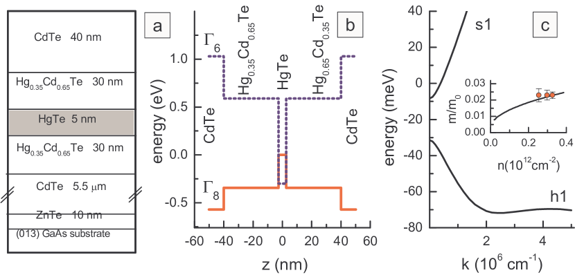
Figure 1: (Color online) (Color online) Architecture (a) and energy diagram (b) of the structure under investigation. (c) The dispersion for the lowest electron (s1) and highest hole (h1) subbands calculated in the framework of isotropic $6\times 6$ kP model. The inset shows the electron density dependence of the effective mass for the electron subband s1. Symbols plot the data, and the line shows the calculated dependence.

III Results and discussion

The gate voltage ($V_{g}$) dependence of the electron density (found both from the Hall effect and from the SdH oscillations) and conductivity are plotted in Figs. 2(a) and 2(b). One can see that $n$ linearly changes with $V_{g}$ with the rate $dn/dV_{g}$ of about $(4.1\pm 0.1)\times 10^{10}$ cm^-2V^-1. This rate is close to $C/e$, where $C$ is specific capacitance measured between the gate electrode and 2D gas for the same structure. As seen we were able to change the conductivity from $5\,G_{0}$ to $120\,G_{0}$ in our $V_{g}$ range.

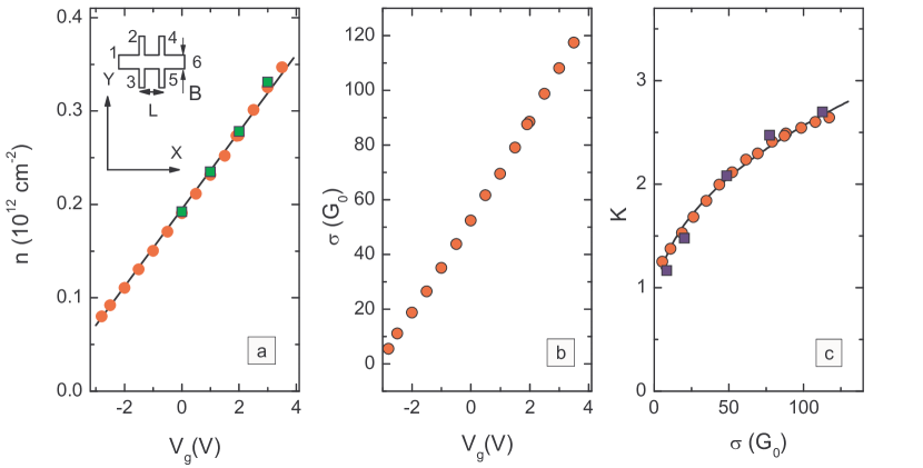
Figure 2: (Color online) The gate voltage dependences of (a) electron density and (b) conductivity obtained from the measurements on the standard Hall bar, shown in the inset. Circles and squares in panel (a) are data obtained from the Hall and SdH effect, respectively. (c) The conductivity dependences of the conductivity anisotropy obtained from the measurements of nonlocal conductivity (squares) and from the measurements performed on the L-shaped Hall bar (circles). The lines are provided as a guide to the eye.

Because the heterostructures were grown on GaAs substrate with (013) surface orientation, it is naturally to suppose that walls of the HgTe quantum well are not ideal plane and can be corrugated. For thin quantum wells (for our case the nominal quantum well width consists of only of $7-8$ lattice constants) such corrugation can result in the anisotropy of conductivity. Therefore, let us consider the results concerning the conductivity anisotropy before to analyze the interference induced magnetoresistivity quantitatively. They have been obtained by two methods.

The first method is based on measurements of the nonlocal conductance on the standard Hall bar. When the principal axes $x$ and $y$ of the conductivity tensor coincide with axes $X$ and $Y$ of the sample coordinate system [see the inset in Fig. 2(a)] the conductivity anisotropy $K=\sigma_{xx}/\sigma_{yy}$ can be found from the ratio of nonlocal conductance ($G_{nL}$) to the local one ($G_{L}$):Germanenko and Minkov (1990)

$$\frac{G_{nL}}{G_{L}}=\frac{4\sqrt{K}}{\pi}\exp\left(-\frac{L}{B}\frac{\pi}{\sqrt{K}}\right),$$ (1)

where $B$ and $L$ stand for the width of the Hall bar and for the distance between probes $3$ and $5$, respectively, $G_{L}=I_{16}/V_{35}$ ($I_{16}/V_{24}$), $G_{nL}=I_{23}/V_{45}$ with $I_{ik}$ as the current flowing through the probes $i$ and $k$, and $V_{lm}$ as the voltage drop between the probes $l$ and $m$.

The conductivity dependence of $K$ measured by this method is plotted by squares in Fig. 2(c). It is seen that the conductivity anisotropy increases with the increase of the conductivity and electron density, and it reaches the value of $K\simeq 2.7$ at $\sigma=120\,G_{0}$ ($n=3.5\times 10^{11}$ cm^-2). Of course, such a dependence may result from an extended mechanical defects, such as scratches or notches, directed along the bar. To make sure that it is not the case and the anisotropy of the conductivity is the physical property of 2D electron gas in the structures investigated, we used the second method.

The anisotropy value in the second method is obtained from the measurements performed on the L-shaped Hall bar (see the inset in Fig. 3), which is made on the basis of the same wafer in such a way that the orientation of arm $1$ on the wafer coincides with the orientation of the Hall bar shown in the inset in Fig. 2(a). Such measurements show that the electron densities in both arms are equal to each other with the accuracy better than $3$%, but the conductivity of arm $1$ ($\sigma_{1}=I_{ab}/V_{ef}\times L/B=\sigma_{xx}$) is significantly higher than that of arm $2$ ($\sigma_{2}=I_{ab}/V_{cd}\times L/B=\sigma_{yy}$) as shown in Fig. 3. The ratio $\sigma_{1}/\sigma_{2}=\sigma_{xx}/\sigma_{yy}=K$ plotted against the conductivity of arm $1$ in Fig. 2(c) shows that the $K$ values obtained by this method practically coincide with those obtained by the first method.

Thus, the conductivity of electron gas in the studied heterostructures with narrow HgTe quantum well grown on (013) substrate is strongly anisotropic that should be taken into account at analysis of transport properties of such type structures.

We are now in a position to consider the low field magnetoconductivity. The magnetic field dependence of $\sigma_{1}$ and $\sigma_{2}$ measured for both arms of L-shaped Hall bar at $T=1.4$ K and $V_{g}=0$ V are presented in Fig. 4(a). Qualitatively, these dependences are analogous. The conductivity decreases in the low magnetic field, reaches the minimum near $B\simeq 60$ mT and increases at higher magnetic field. Such a behavior is typical for the interference induced magnetoconductivity for the case of fast spin relaxation, $\tau_{s}<\tau_{\phi}$, where $\tau_{s}$ is the spin relaxation time. Notice that the magnitude of the magnetoconductivity $\Delta\sigma_{1}(B)=\sigma_{1}(B)-\sigma_{1}(0)$ and $\Delta\sigma_{2}(B)=\sigma_{2}(B)-\sigma_{2}(0)$ is different whereas the characteristic magnetic field scales are the same; $\sigma_{2}$ being multiplied by the factor close to two coincides practically with $\sigma_{1}$ as illustrated by solid line in Fig. 4(a).

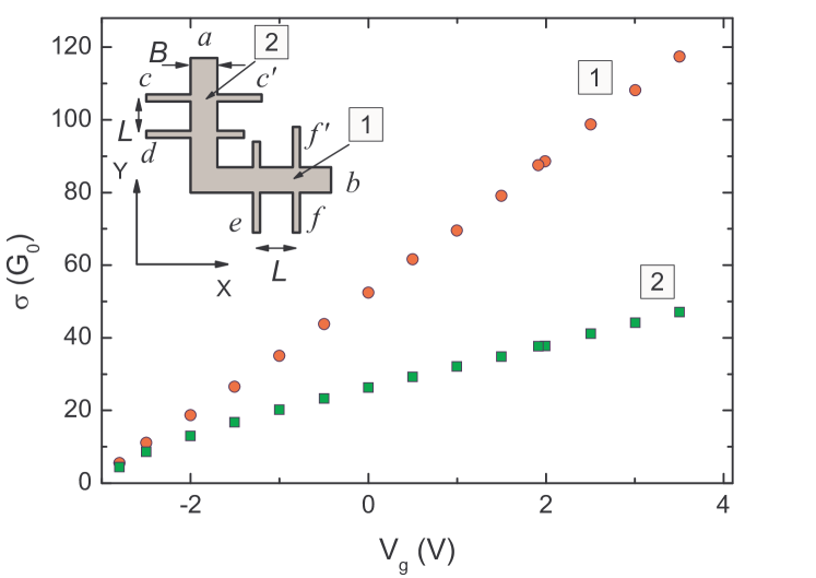
Figure 3: The gate voltage dependence of the conductivity measured on the different arms of the L-shaped Hall bar shown in the inset.

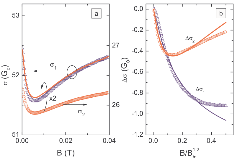
Figure 4: The dependences of (a) $\sigma_{1,2}(B)$ and (b) $\Delta\sigma_{1,2}(B/B_{tr}^{1,2})$ for the L-shaped Hall bar measured for $V_{g}=0$ V at $T=1.4$ K. $B_{tr}^{1}=0.014$ T, $B_{tr}^{2}=0.056$ T. The curve in the panel (a) is $\sigma_{2}(B)\times K=\sigma_{2}(B)\sigma_{1}(0)/\sigma_{2}(0)=2\,\sigma_{2}(B)$. The curves in the panel (b) are the results of the best fit by Eq. (2) with the parameters given in the text.

Theoretically, the weak localization and antilocalization for narrow gap ($d\simeq d_{c}$) HgTe quantum wells is comprehensively studied in Ref. Ostrovsky et al., 2012. The effective HamiltonianBernevig et al. (2006) is used to describe the spectrum of the 2D gas. The authors show that the magnetoconductivity can be positive or negative or it can demonstrate alternative-sign behavior with the increasing magnetic field. Which scenario is realized, it depends on the position of the Fermi level as illustrated in Ref. Ostrovsky et al., 2012 by Fig. 1. For our samples, the Fermi level lies in the linear part of the spectrum. The Fermi energy equal to ($25-55$) meV for different $V_{g}$ is always larger than the value of $m(k_{F})\simeq(15-20)$ meV [$m(k_{F})$ is introduced by Eq. (4) in Ref. Ostrovsky et al., 2012]. For such the case the 1Sp$\to$2U scenario should be realized with the growing magnetic field according to Ref. Ostrovsky et al., 2012. This means that the magnetoconductivity being negative in the low field has to saturate in the higher one. As seen from Fig. 4 the experimental picture of the magnetoconductivity is somewhat different. The magnetoconductivity is really negative in the low magnetic field, $B\lesssim 60$ mT. However, in the higher magnetic field the rise of the conductivity is observed instead of the saturation. In Ref. Ostrovsky et al., 2012, such a behavior (characteristic to the pattern 1Sp$\to$2O) was predicted only for very low and very large concentrations of carriers, corresponding to the strong nonlinearity of the spectrum. The difference apparently results from the fact that only the diffusion (logarithmic) contributions to the interference quantum correction have been taken into account in Ref. Ostrovsky et al., 2012. As seen from Fig. 4 the rise of the conductivity is evident in the magnetic field which is not very small as compared with the characteristic for weak localization transport magnetic field, $B_{tr}=\hbar/4eD\tau$, where $\tau$ is the transport relaxation time and $D$ is the diffusion constant. This indicates that the ballistic contribution which also depend on magnetic field may play significant role in the actual case. Indeed, when the leading logarithmic contributions cancel each other (regime 2U), the subleading ballistic terms may dominate the magnetic-field dependence of the interference correction to the conductivity. In fact, the magnitude of the negative magnetoresistance in Fig. 4 does not exceed $G_{0}$ and can therefore result from the ballistic effects.

Thus, unfortunately the expressions from Ref. 15 cannot be applied to analyze our data quantitatively in the whole range of magnetic fields. There is a clear need of a theoretical description of magnetoconductivity in HgTe structures in a whole range of magnetic fields including ballistic effects. Therefore, we will follow traditional way using the Hikami-Larkin-Nagaoka (HLN) expressionHikami et al. (1980); Knap et al. (1996) to describe the interference induced magnetoconductivity:

$$\Delta\sigma(B)=G_{0}{\cal H}\left(\frac{B}{B_{tr}},\frac{\tau}{\tau_{\phi}},\frac{\tau}{\tau_{s}}\right),$$ (2)

where

$${\cal H}(b,x,y) = \psi\left(\frac{1}{2}+\frac{x+y}{b}\right)-\ln{\left(x+y\right)}$$

$$+ \frac{1}{2}\psi\left(\frac{1}{2}+\frac{x+2y}{b}\right)-\frac{1}{2}\ln{\left(x+2y\right)}$$

$$- \frac{1}{2}\psi\left(\frac{1}{2}+\frac{x}{b}\right)+\frac{1}{2}\ln{\left(x\right)}-\psi\left(\frac{1}{2}+\frac{1}{b}\right)$$

with $\psi(x)$ as a digamma function.

Let us firstly analyze the data obtained on the two arms by the standard manner as if they have been obtained on the two different samples with isotropic conductivity. The results of the best fit made within the magnetic field range $B/B_{tr}^{1,2}=0-0.3$ ($B_{tr}^{1}=0.014$ T, $B_{tr}^{2}=0.056$ T) for each arm are presented in Fig. 4(b). The figure shows a good fit of the equation to the data. Nevertheless, the values of the fitting parameters are different. While the difference between the $\tau_{\phi}$ values for the arms 1 and 2 is not very large ($\tau_{\phi}^{1}=3.8\times 10^{-11}$ s and $\tau_{\phi}^{2}=3.2\times 10^{-11}$ s), the difference between $\tau_{s}^{1}$ and $\tau_{s}^{2}$ is significant: $\tau_{s}^{1}=0.9\times 10^{-12}$ s is approximately five times smaller than $\tau_{s}^{2}=4.7\times 10^{-12}$ s. In what follows we show that the reason for such a discrepancy is neglect of the conductivity anisotropy in the above data analysis.

The interference correction to the conductivity of the 2D anisotropic systems was studied in Refs. Wölfle and Bhatt, 1984; Bhatt et al., 1985. If one follows this line of attack, the interference induced magnetoconductivity can be written within the diffusion approximation, $\tau_{\phi}$, $\tau_{s}\gg\tau$, in the form:

$$\Delta\sigma_{xx}(B) = \sqrt{K}\,G_{0}\,{\cal H}\left(\frac{B}{B^{\prime}_{tr}},\frac{\tau^{\prime}}{\tau_{\phi}},\frac{\tau^{\prime}}{\tau_{s}}\right)$$

$$\Delta\sigma_{yy}(B) = \frac{1}{\sqrt{K}}\,G_{0}\,{\cal H}\left(\frac{B}{B^{\prime}_{tr}},\frac{\tau^{\prime}}{\tau_{\phi}},\frac{\tau^{\prime}}{\tau_{s}}\right),$$ (3)

where $B^{\prime}_{tr}=\sqrt{B_{tr}^{1}B_{tr}^{2}}$ and $\tau^{\prime}=\sqrt{\tau_{1}\tau_{2}}$.

Thus, the values of $\Delta\sigma_{1}/\sqrt{K}$ and $\Delta\sigma_{2}\sqrt{K}$ plotted as functions of $B/B^{\prime}_{tr}$ should coincide and they should be described by the expression, Eq. (2), with $b=B/B^{\prime}_{tr}$, $x=\tau^{\prime}/\tau_{\phi}$, and $y=\tau^{\prime}/\tau_{s}$. As evident from Fig. 5 the experimental data for the arms 1 and 2 replotted in such the manner are really close to each other, but, what is more important, we obtain the very close parameters for two arms: $\tau_{\phi}=3.8\times 10^{-11}$ s, $3.5\times 10^{-11}$ s and $\tau_{s}=3.1\times 10^{-12}$ s, $3.2\times 10^{-12}$ s for arms $1$ and $2$, respectively. Existing difference between the data for different arms and between the corresponding fitting parameters may result from the fact that the diffusion regime, $\tau\ll\tau_{s},\,\tau_{\phi}$, is not strictly realized under our experimental conditions; $\tau_{s}$ is only seventeen times larger than $\tau^{\prime}$.

It is pertinent to note here that the $\tau_{\phi}$ values are very close to each other independently of that how they have been obtained. Considering the arms 1 and 2 as independent isotropic samples and taking into account the conductivity anisotropy we have obtained practically the same results: $\tau_{\phi}=(3.2-3.8)\times 10^{-11}$ s. As for the spin relaxation time, the ignoring of the conductivity anisotropy when treating the data can give an error in $\tau_{s}$ of several times of magnitude.

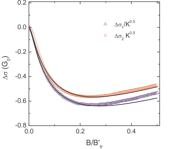
Figure 5: The values of $\Delta\sigma_{1}/\sqrt{K}$ and $\Delta\sigma_{2}\sqrt{K}$ plotted as functions of $B/B^{\prime}_{tr}$, $B^{\prime}_{tr}=0.028$ T, for $V_{g}=0$ V and $T=1.4$ K. The symbols are the data, the solid lines are the result of the best fit by Eq. (2) with the parameters given in the text.

Now, making sure that Eq. (3) for the interference correction in anisotropic 2D system describes the experimental data adequately we can proceed to analysis of the dependences of the parameters $\tau_{\phi}$ and $\tau_{s}$ on the temperature and conductivity.

The temperature dependences of $\tau_{\phi}$ and $\tau_{s}$ for two gate voltages are depicted in Fig. 6. One can see that the $T$ dependences of $\tau_{\phi}$ obtained for each of the arms coincide very closely. They are well described by the $1/T$ law that is consistent with theoretical prediction for the case when the phase relaxation is determined by inelasticity of electron-electron (e-e) interaction.Altshuler and Aronov (1985) The spin relaxation time is practically independent of the temperature as it should be for the degenerate gas of carriers. Such dependences of the fitting parameters $\tau_{\phi}$ and $\tau_{s}$ support using of the HLN expression for description of interference induced magnetoresistance.

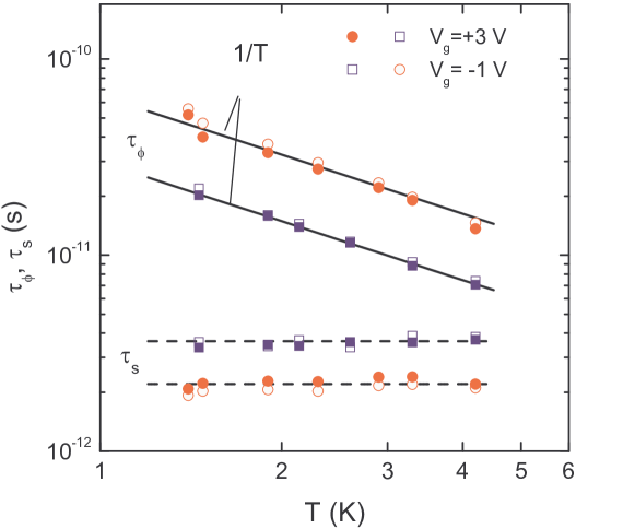
Figure 6: The temperature dependences of $\tau_{\phi}$ and $\tau_{s}$ for two gate voltages, $V_{g}=-1$ V and $3$ V. Solid and open symbols plot the data obtained from analysis of the dependences $\Delta\sigma_{1}(B)/\sqrt{K}$ and $\Delta\sigma_{2}(B)\sqrt{K}$, respectively. The dashed lines are provided as a guide to the eye.

Let us now consider the main result of the paper. It is the conductivity dependence of the phase relaxation time shown in Fig. 7, where $\sigma^{\prime}=\sqrt{\sigma_{1}\sigma_{2}}$. It is evident that $\tau_{\phi}$ found experimentally increases with the increasing conductivity. Such the behavior is analogous to that observed in quantum wells with ordinary spectrum (see, e.g., Ref. Minkov et al., 2004, where the data for GaAs/In_0.2Ga_0.8As/GaAs quantum well are presented). Our data are in satisfactory agreement with the theoretical results obtained in Ref. Zala et al., 2001 for the usual 2D systems for the case when inelasticity of e-e interaction is the main mechanism of phase relaxation. This is clearly seen from Fig. 7, where the curves represent the calculation results for two values of the parameter e-e interaction $F_{0}^{\sigma}$: $F_{0}^{\sigma}=0$ and $-0.5$. Note, the fact that most of the experimental points fall between the theoretical curves cannot be regarded as a method of determining $F_{0}^{\sigma}$ vs $\sigma$ dependence in these systems.

The growing $\tau_{\phi}$ vs $\sigma$ dependence observed in the present paper for the narrow quantum well, $d=5$ nm, with normal energy spectrum differs drastically from that obtained in Ref. Minkov et al., 2012 by the same method for the structures with the wider quantum well, $d=(9-10)$ nm, with the inverted subband ordering. The results from Ref. Minkov et al., 2012 are presented in Fig. 7 also. As seen $\tau_{\phi}$ is practically independent of the conductivity in the quantum well with inverted spectrum in contrast to the data obtained for the wells with normal spectrum.

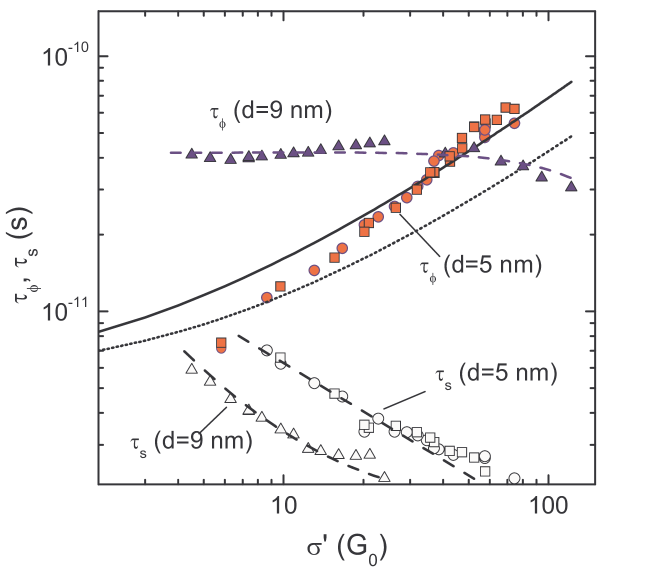
Figure 7: The conductivity dependence of $\tau_{\phi}$ and $\tau_{s}$ for HgTe quantum well with inverted ($d=9$ nm) and normal ($d=5$ nm) energy spectrum obtained in Ref. Minkov et al., 2012 and this paper, respectively. The solid and dotted lines are calculated according to Ref. Zala et al., 2001 with $F_{0}^{\sigma}=0$ and $-0.5$, respectively. The dashed lines are provided as a quid to the eye.

Thus, the fitting parameter $\tau_{\phi}$ identifying with the phase relaxation time behaves itself with increasing $\sigma$ in narrow quantum well HgTe with normal subband ordering in the same way as in usual 2D systems. When we are dealing with the electrons in the inverted band, the $\tau_{\phi}$ vs $\sigma$ behavior is extraordinary. As was discussed in Ref. Minkov et al., 2012 one of the possible reason for the latter case is that the fitting parameters $\tau_{\phi}$ and $\tau_{s}$ may not correspond to the true phase and spin relaxation times, respectively, despite the fact that the standard HLN expression fits the experimental magnetoconductivity curves rather well. We presume that this could result from the fact that the HLN expression does not take into account a multi-component character of the electron wave functions. Because electrons in narrow ($d<d_{c}$) and wide ($d>d_{c}$) HgTe quantum wells belong to the different branches of the spectrumGerchikov and Subashiev (1990); Bernevig et al. (2006) with sufficiently different structures of the wave functions, the effects of electron interference can in principle be strongly dependent on the width of quantum well, which controls the subband ordering.

Strictly speaking, the above allowance for the conductivity anisotropy is rigorous in the case when the electric current flows along the principal axes of the conductivity tensor. We show in the supplemental material that the measurements performed on the L-shaped Hall bar allow ones to find the principal exes of the conductivity tensor and, thus, perform the analysis of the magnetoconductivity for the arbitrary orientation of the bar and conductivity tensor. It is shown that misorientation between the conductivity tensor and the Hall bar is small enough so that the taking it into account is not needed in our concrete case.

IV Conclusion

Investigating the interference induced magnetoconductivity in narrow HgTe single quantum well we have shown that the phase relaxation time found from the fit of the low-field magnetoconductivity for the quantum well with the normal energy spectrum increases with the conductivity increase analogously to that observed in ordinary single quantum wells. Such the behavior is in agreement with that predicted theoretically for the case when inelasticity of e-e interaction is the main mechanism of the phase relaxation time. At the same time, it differs markedly from the behavior of $\tau_{\phi}$ obtained in wider HgTe quantum well with inverted energy spectrum,Minkov et al. (2012) where $\tau_{\phi}$ is nearly constant over the wide conductivity range. It is proposed that different structure of the multicomponent electron wave functions for $d<d_{c}$ and $d>d_{c}$ could be responsible for such a discrepancy.

Supplemental Material

Analysis in the paper is performed under assumption that the principal axes $x$ and $y$ of the conductivity tensor coincide with the axes $X$ and $Y$ of the coordinate system connected with sample as shown in Fig. 2(a) and Fig. 3. If it is not the case, i.e., the angle $\theta$ between the $X$ and $x$ axes is nonzero (see the inset in Fig. 8), the $\sigma_{xx}$ and $\sigma_{yy}$ components as well as the $\theta$ angle can be found from resolving the following system of equations:

$$\sigma_{1}^{-1} = \sigma^{-1}_{xx}(\cos{\theta})^{2}+\sigma^{-1}_{yy}(\sin{\theta})^{2}$$

$$\sigma_{2}^{-1} = \sigma^{-1}_{xx}(\sin{\theta})^{2}+\sigma^{-1}_{yy}(\cos{\theta})^{2}$$

$$V_{cc^{\prime}} = \frac{1}{2}I_{ab}(\sigma^{-1}_{xx}-\sigma^{-1}_{yy})\sin{2\theta}$$

$$V_{f^{\prime}f} = V_{cc^{\prime}},$$ (4)

where the current $I_{ab}$ flowing through the probes $a$ and $b$, and the quantities $\sigma_{1}$, $\sigma_{2}$, and $V_{cc^{\prime}}$ (or $V_{f^{\prime}f}$) are measured experimentally. Doing so we have obtained $\theta=(22\pm 5)^{\circ}$, and $\sigma_{xx}$, $\sigma_{yy}$ plotted against the gate voltage in Fig. 8. One can see that the data obtained are consistent with the results obtained in the main paper; $\sigma_{xx}>\sigma_{1}$ while $\sigma_{yy}<\sigma_{2}$ so that $\sigma_{xx}/\sigma_{yy}>\sigma_{1}/\sigma_{2}$.

As for the interference induced magnetoconductivity measured on the L-shaped Hall, it is easy to show that the following expression is valid for $\Delta\sigma_{1,2}(B)$:

$$\Delta\sigma_{1}(B) = \sqrt{\frac{\sigma_{1}}{\sigma_{2}}}\,G_{0}\,{\cal H}\left(\frac{B}{B^{\prime}_{tr}},\frac{\tau^{\prime}}{\tau_{\phi}},\frac{\tau^{\prime}}{\tau_{s}}\right)F(K,\theta),$$

$$\Delta\sigma_{2}(B) = \sqrt{\frac{\sigma_{2}}{\sigma_{1}}}\,G_{0}\,{\cal H}\left(\frac{B}{B^{\prime}_{tr}},\frac{\tau^{\prime}}{\tau_{\phi}},\frac{\tau^{\prime}}{\tau_{s}}\right)F(K,\theta),$$ (5)

where $K=\sigma_{xx}/\sigma_{yy}$ and

$$F(K,\theta)=\sqrt{\frac{K}{\left(\sin^{2}\theta+K\cos^{2}\theta\right)\left(K\sin^{2}\theta+\cos^{2}\theta\right)}}.$$ (6)

Thus, the experimental dependences $\Delta\sigma_{1}(B)\sqrt{\sigma_{2}/\sigma_{1}}$ and $\Delta\sigma_{2}(B)\sqrt{\sigma_{1}/\sigma_{2}}$ measured for arbitrary orientation of the L-shaped Hall should be described by the same function ${\cal H}(b,x,y)$ multiplied by the factor $F(K,\theta)$ given by Eq. (6).

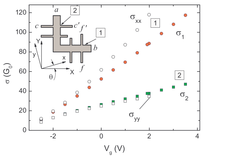
Figure 8: The gate voltage dependence of $\sigma_{1}$ and $\sigma_{2}$ measured for arms $1$ and $2$ (solid symbols) as compared with that of $\sigma_{xx}$ and $\sigma_{yy}$, found as described in the text. The inset illustrates the orientation of the principal axes $x$ and $y$ of the conductivity tensor in the coordinate system of the sample.

If one uses $\theta=22^{\circ}$ and maximal under our conditions value of $K$, $K=4$, one obtains $F(K,\theta)\simeq 0.9$. Because this value is close to one, it is obviously that ignoring $F(K,\theta)$ in the main text does not affect the results of the paper. It is justified by the direct inclusion of the factor $F(K,\theta)$ into the fitting procedure. Taking the factor $F(K,\theta)$ into account results in the maximal increase of $\tau_{\phi}$ by approximately $2$ % and decrease of $\tau_{s}$ by $20$ % or less over the entire temperature and conductivity ranges used in the paper.

References

- Volkov and Pinsker (1976) V. A. Volkov and T. N. Pinsker, Zh. Eksp. Teor. Fiz. 70, 2268 (1976), [Sov. Phys. JETP 43, 1183 (1976)].
- Dyakonov and Khaetskii (1982) M. I. Dyakonov and A. Khaetskii, Zh. Eksp. Teor. Fiz. 82, 1584 (1982), [Sov. Phys. JETP 55, 917 (1982)].
- Lin-Liu and Sham (1985) Y. R. Lin-Liu and L. J. Sham, Phys. Rev. B 32, 5561 (1985).
- Gerchikov and Subashiev (1990) L. G. Gerchikov and A. Subashiev, Phys. Stat. Sol. (b) 160, 443 (1990).
- Bernevig et al. (2006) B. A. Bernevig, T. L. Hughes, and S.-C. Zhang, Science 314, 1757 (2006).
- Landwehr et al. (2000) G. Landwehr, J. Gerschütz, S. Oehling, A. Pfeuffer-Jeschke, V. Latussek, and C. R. Becker, Physica E 6, 713 (2000).
- Zhang et al. (2002) X. C. Zhang, A. Pfeuffer-Jeschke, K. Ortner, C. R. Becker, and G. Landwehr, Phys. Rev. B 65, 045324 (2002).
- Ortner et al. (2002) K. Ortner, X. C. Zhang, A. Pfeuffer-Jeschke, C. R. Becker, G. Landwehr, and L. W. Molenkamp, Phys. Rev. B 66, 075322 (2002).
- Zhang et al. (2004) X. C. Zhang, K. Ortner, A. Pfeuffer-Jeschke, C. R. Becker, and G. Landwehr, Phys. Rev. B 69, 115340 (2004).
- König et al. (2007) M. König, S. Wiedmann, C. Brüne, A. Roth, H. Buhmann, L. W. Molenkamp, X.-L. Qi, and S.-C. Zhang, Science 318, 766 (2007).
- Gusev et al. (2011) G. M. Gusev, Z. D. Kvon, O. A. Shegai, N. N. Mikhailov, S. A. Dvoretsky, and J. C. Portal, Phys. Rev. B 84, 121302 (2011).
- Kvon et al. (2011) Z. D. Kvon, E. B. Olshanetsky, E. G. Novik, D. A. Kozlov, N. N. Mikhailov, I. O. Parm, and S. A. Dvoretsky, Phys. Rev. B 83, 193304 (2011).
- Tkachov and Hankiewicz (2011) G. Tkachov and E. M. Hankiewicz, Phys. Rev. B 84, 035444 (2011).
- Nicklas and Wilkins (2011) J. W. Nicklas and J. W. Wilkins, Phys. Rev. B 84, 121308 (2011).
- Ostrovsky et al. (2012) P. M. Ostrovsky, I. V. Gornyi, and A. D. Mirlin, Phys. Rev. B 86, 125323 (2012).
- Olshanetsky et al. (2010) E. B. Olshanetsky, Z. D. Kvon, G. M. Gusev, N. N. Mikhailov, S. A. Dvoretsky, and J. C. Portal, Pis’ma Zh. Eksp. Teor. Fiz. 91, 375 (2010), [JETP Letters 91, 347 (2010)].
- Minkov et al. (2012) G. M. Minkov, A. V. Germanenko, O. E. Rut, A. A. Sherstobitov, S. A. Dvoretski, and N. N. Mikhailov, Phys. Rev. B 85, 235312 (2012).
- Mikhailov et al. (2006) N. N. Mikhailov, R. N. Smirnov, S. A. Dvoretsky, Y. G. Sidorov, V. A. Shvets, E. V. Spesivtsev, and S. V. Rykhlitski, Int. J. Nanotechnology 3, 120 (2006).
- Larionova and Germanenko (1996) V. A. Larionova and A. V. Germanenko, Phys. Rev. B 55, 13062 (1996).
- Zhang et al. (2001) X. C. Zhang, A. Pfeuffer-Jeschke, K. Ortner, V. Hock, H. Buhmann, C. R. Becker, and G. Landwehr, Phys. Rev. B 63, 245305 (2001).
- Novik et al. (2005) E. G. Novik, A. Pfeuffer-Jeschke, T. Jungwirth, V. Latussek, C. R. Becker, G. Landwehr, H. Buhmann, and L. W. Molenkamp, Phys. Rev. B 72, 035321 (2005).
- Note (1) It should be mentioned that not only the corrugation of the HgTe/Hg1-xCdxTe interfaces may result in the conductivity anisotropy. Anisotropy can be of technological origin. For instance, the quasiperiodic structure of different composition of solid solution Hg1-xCdxTe can be formed during epitaxial growth under certain conditions as shown in Ref. \rev@citealpnumSabinina11. This modulated composition can also result in anisotropy of electrical properties.
- Germanenko and Minkov (1990) A. V. Germanenko and G. M. Minkov, Solid State Commun. 74, 649 (1990).
- Hikami et al. (1980) S. Hikami, A. I. Larkin, and Y. Nagaoka, Prog. Theor. Phys. 63, 707 (1980).
- Knap et al. (1996) W. Knap, A. Zduniak, L. H. Dmowski, S. Contreras, and M. I. Dyakonov, Phys. Stat. Sol. (b) 198, 267 (1996).
- Wölfle and Bhatt (1984) P. Wölfle and R. N. Bhatt, Phys. Rev. B 30, 3542 (1984).
- Bhatt et al. (1985) R. N. Bhatt, P. Wölfle, and T. V. Ramakrishnan, Phys. Rev. B 32, 569 (1985).
- Altshuler and Aronov (1985) B. L. Altshuler and A. G. Aronov, in Electron-Electron Interaction in Disordered Systems, edited by A. L. Efros and M. Pollak (North Holland, Amsterdam, 1985) p. 1.
- Minkov et al. (2004) G. M. Minkov, A. V. Germanenko, and I. V. Gornyi, Phys. Rev. B 70, 245423 (2004).
- Zala et al. (2001) G. Zala, B. N. Narozhny, and I. L. Aleiner, Phys. Rev. B 64, 214204 (2001).
- Sabinina et al. (2011) I. Sabinina, A. Gutakovsky, Y. G. Sidorov, and A. Latyshev, Pis’ma Zh. Eksp. Teor. Fiz. 94, 348 (2011), [JETP Letters 94, 324 (2011)].