Synchronization of a Josephson junction array in terms of global variables

Abstract

We consider an array of Josephson junctions with a common LCR-load. Application of the Watanabe-Strogatz approach [Physica D, v. 74, p. 197 (1994)] allows us to formulate the dynamics of the array via the global variables only. For identical junctions this is a finite set of equations, analysis of which reveals the regions of bistability of the synchronous and asynchronous states. For disordered arrays with distributed parameters of the junctions, the problem is formulated as an integro-differential equation for the global variables, here stability of the asynchronous states and the properties of the transition synchrony-asynchrony are established numerically.

I Introduction

Synchronization in populations of coupled oscillators is a general phenomenon observed in many physical systems, see recent experimental studies of optomechanical, micromechanical, electronic, mechanical, chemical oscillators  Heinrich et al. (2011); *Zhang_etal-12; *Temirbayev_etal-12; *Martens_etal-13; *Tinsley_etal-12. Synchronization effects are also ubiquitous in biology and social sciences. One of the basic examples of oscillating physical systems that being coupled synchronize, are Josephson junctions Jain et al. (1984); *Benz-Burroughs-91; *Whan-Cawthorne-Lobb-96; *Cawthorne_etal-99. In theoretical studies of the Josephson junction arrays one typically either performs direct numerical simulation of the microscopic equations (see, e.g., Hadley et al. (1988); *Filatrella_etall-00) or reduces the problem to the standard Kuramoto-type model Wiesenfeld and Swift (1995); Wiesenfeld et al. (1996, 1998).

Quite remarkable in this respect is the paper Heath and Wiesenfeld (2000), where a careful comparison of the microscopic modeling and the reduced Kuramoto-type model has been performed. The authors demonstrated that a hysteretic transition to synchrony in an array of Josephson junctions can be explained by a Kuramoto-type modeling (where usually the transition is not hysteretic), if in its derivation one self-consistently accounts for changes of the oscillator parameters.

Our aim in this paper is to shed light on the hysteretic transitions to synchrony in Josephson arrays by studying the equations for global variables. In this approach, that is based on the seminal papers by Watanabe and Strogatz (WS) Watanabe and Strogatz (1993, 1994), it is possible to formulate exact low-dimensional equations for the array, without using approximate reduction to the Kuramoto model. The paper is organized as follows. First, we formulate the equations for the array of identical junctions via the global variables. Analysis of these equations shows regions of bistability asynchrony–synchrony, and the hysteretic transitions. Then we proceed to non-identical junctions, where the equations are of more complex form. Here we analyze stability of asynchronous states, and show numerically that the transition to synchrony is also hysteretic.

II Identical Junctions

II.1 Formulation in terms of global variables

We start with formulating the system of equations for the Josephson junction series array with a LCR load. Our setup is the same as in refs. Wiesenfeld and Swift (1995); Wiesenfeld et al. (1996, 1998), the equatons for the junction phases $\varphi_{i}$ and the load capacitor charge $Q$ read

$${\hbar\over 2er}\frac{d\varphi_{i}}{dt}+I_{c}\sin\varphi_{i} =I-\frac{dQ}{dt}\;,$$ (1)

$$L\frac{d^{2}Q}{dt^{2}}+R\frac{dQ}{dt}+\frac{Q}{C} ={\hbar\over 2e}\sum_{i=1}^{N}\frac{d\varphi_{i}}{dt}\;.$$

Here $N$ is the number of junctions, described by a resistive model with critical current $I_{c}$ and resistance $r$, while $L,C,R$ are parameters of the LCR-load. It is convenient to introduce dimensionless variables according to

$$\begin{gathered}\omega_{c}=2erI_{c}/\hbar,\ \ t^{*}=\omega_{c}t,\\ \ \ Q^{*}=\omega_{c}L^{*}Q/I_{c},\ \ I^{*}=I/I_{c},\\ R^{*}=R/rN,\ \ L^{*}=\omega_{c}L/rN,\ \ C^{*}=N\omega_{c}rC\;,\end{gathered}$$ (2)

and to rewrite the system (1) in a dimensionless form (droping asterixes for simplicity)

$$\dot{\varphi_{i}} =I-\epsilon\dot{Q}-\sin\varphi_{i},$$ (3)

$$\ddot{Q}+\gamma\dot{Q}+\omega_{0}^{2}Q =I-{1\over N}\sum_{i=1}^{N}\sin\varphi_{i},$$

where $\epsilon=1/L^{*}$, $\gamma=(R^{*}+1)/L^{*}$, and $\omega_{0}=1/\sqrt{L^{*}C^{*}}$.

The global coupling can be represented through the complex mean field (Kuramoto order parameter)

$$Z=re^{\text{i}\theta} ={1\over N}\sum_{i=1}^{N}(\cos\varphi_{i}+\text{i}\sin\varphi_{i})\;,$$ (4)

$${\rm Im}(Z) ={1\over N}\sum_{i=1}^{N}\sin\varphi_{i}\;,$$

and the equations for the junction phases can be written as

$$\dot{\varphi_{i}}=I-\epsilon\dot{Q}+{\rm Im}(e^{-\text{i}\varphi_{i}}).$$ (5)

This form of the phase equation allows us to use the Watanabe-Strogatz ansatz Watanabe and Strogatz (1993, 1994), applicable to general systems of phase equations driven by a common force and having form

$$\dot{\varphi_{i}}=f(t)+{\rm Im}(G(t)e^{-\text{i}\varphi_{i}})$$ (6)

with arbitrary real $f(t)$ and complex $G(t)$ (in our case $f=I-\epsilon\dot{Q}$, $G=1$). We use the formulation of the Watanabe-Strogatz theory presented in Ref. Pikovsky and Rosenblum (2011). The ensemble is characterized by three global time-dependent WS variables $\rho,\Phi,\Psi$ and $N$ constants of motion $\psi_{i}$ (of which only $N-3$ are independent) which are related to the phases $\varphi_{i}$ as

$$e^{\text{i}\varphi_{i}}=e^{\text{i}\Phi}\frac{\rho+\exp(\text{i}(\psi_{i}-\Psi))}{\rho\exp(\text{i}(\psi_{i}-\Psi))+1}$$ (7)

with additional conditions $\sum_{i}\cos\psi_{i}=\sum_{i}\sin\psi_{i}=\sum_{i}\cos 2\psi_{i}=0$. The equations for the global WS variables read Watanabe and Strogatz (1993, 1994); Pikovsky and Rosenblum (2011)

$$\dot{\rho} =\frac{1-\rho^{2}}{2}{\rm Re}(e^{-\text{i}\Phi}),$$ (8)

$$\dot{\Psi} =\frac{1-\rho^{2}}{2\rho}{\rm Im}(e^{-\text{i}\Phi}),$$

$$\dot{\Phi} =I-\epsilon\dot{Q}+\frac{1+\rho^{2}}{2\rho}{\rm Im}(e^{-\text{i}\Phi}).$$

To close the system we need to add the equation for $Q$, where the imaginary part of the order parameter $Z$ enters, so $Z$ should be represented through the Watanabe-Strogatz variables. In general, the expression for $Z$ is rather complex (cf. Pikovsky and Rosenblum (2008, 2011)) but in the case of a uniform distribution of the constants $\psi_{i}$, the order parameter is just $Z=\rho e^{\text{i}\Phi}$. This important case, where WS global variables $\rho,\Phi$ have a clear physical meaning as the components of the Kuramoto order parameter, will be treated below. Additionally, we notice that the variable $\Psi$ does not enter other equations, so we obtain a closed system of equations that describes the array

$$\dot{Z} =\text{i}(I-\epsilon\dot{Q})Z+{1\over 2}-{Z^{2}\over 2},$$ (9)

$$\ddot{Q}+\gamma\dot{Q}+\omega_{0}^{2}Q =I-{\rm Im}(Z).$$

II.2 Bistability and hysteretic transitions

Analysis of system (9) is our goal in the rest of this section. Before proceeding, some remarks are in order. First, in the derivation of (9) no approximation except for an assumption of a uniform distribution of constants $\psi_{i}$, has been made. The latter is a restriction on initial conditions, we discuss its relevance below. Second, the order parameter $Z$ does not vanish in the case of full asynchrony of junctions: for noncoupled junctions with $\epsilon=0$ we get a steady state $Z_{0}=\text{i}(I-\sqrt{I^{2}-1})$. This non-vanishing value appears because free junctions rotate non-uniformly and the “natural” distribution of the phases in the asynchronous state is not uniform.

We start the analysis of (9) with finding its steady states. Because at such a state $\dot{Q}=0$, the coupling vanishes and the steady state describing the asynchronous regime with $Z_{0}=\text{i}(I-\sqrt{I^{2}-1})$, $Q_{0}=\omega_{0}^{-2}\sqrt{I^{2}-1}$ is the only stationary solution. Stability of this solution is determined by the fourth-order characteristic equation

$$\lambda^{4}+\gamma\lambda^{3} +(\omega_{0}^{2}+I^{2}-1)\lambda^{2}+$$ (10)

$$+[(\gamma-\epsilon)(I^{2}-1) +\epsilon I\sqrt{I^{2}-1}\;]\lambda+\omega_{0}^{2}(I^{2}-1)=0.$$

The stability border can be easily found by assuming $\lambda=\text{i}\omega$:

$$\omega_{0}^{2}=(I^{2}-1)+{\epsilon\over\gamma}\sqrt{I^{2}-1}(I-\sqrt{I^{2}-1}).$$ (11)

The fully synchronous solution of (9) corresponds to the case $|Z|=1$, so that only the phase $\Phi$ changes, according to the system

$$\ddot{Q} +\gamma\dot{Q}+\omega_{0}^{2}Q=I-\sin\Phi\;,$$ (12)

$$\dot{\Phi} =I-\epsilon\dot{Q}-\sin\Phi\;.$$

We have found the limit cycle in Eq. (12) numerically and determined its stability by finding the largest multiplier. Together with expression (11) this allows us to find the domains of stability of the asynchronous and synchronous states, together with the region of bistability of these regimes, see Fig. 1.

Figure 1: (Color online) Domains of stability of synchronous (above lower dashed line) and asynchronous (below upper solid line) states on the plane of parameters ($\omega_{0}^{2},\Omega^{2}$), where $\Omega=\sqrt{I^{2}-1}$ is the natural frequency of the junctions. Here $\epsilon=0.5$, and $\gamma=1.0$ (a), $\;1.7$ (b), $\;2.7$ (c).

In Fig. 2 we give another illustration of the bistability, presenting the dependence of $Z_{0}$ on parameter $I$, together with the value $|Z|=1$ in the synchronous case. Here we also show what happens if our basic assumption at derivation of eqs. (9), namely of a uniform distribution of constants $\psi_{i}$, is not satisfied. We have simulated an ensemble of 100 junctions, preparing the initial conditions with a nonuniform distribution of constants $\psi_{i}$ as described in ref. Pikovsky and Rosenblum (2011), appendix C. Instead of leading to a stable state $Z_{0}$, the desynchronous population now shows an oscillating variable $Z(t)$, minima and maxima of which are marked with squares. In the synchronous regime, $|Z|=1$ as before, and the information on the constants $\psi_{i}$ gets lost as synchrony establishes.

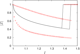
Figure 2: Dependence of the order parameter $|Z|$ on the current $I$ for 100 junctions. Line: uniform distribution of constants $\psi_{i}$, squares: nonuniform distributions.

III Nonidentical Junctions

III.1 Formulation of the model

There are two parameters of individual junctions that can differ: the critical current $I_{c}$ and the resistance $r$ (cf. Wiesenfeld et al. (1996, 1998)). In order to be able to apply the Watanabe-Strogatz approach as above, we will assume that they are organized in groups, each of the size $P$, and the parameters of all junctions in a group are identical: the critical current is $I_{c}(1+\xi_{k})$ and the resistance is $r(1+\eta_{k})$, where index $k=1,\ldots,M$ counts the groups. The total number of junctions is $N=MP$. In this setup the equations for the junctions read

$$\dot{\varphi}_{ki} =(1+\eta_{k})[I-\epsilon\dot{Q}-(1+\xi_{k})\sin\varphi_{ki}]$$ (13)

$$\ddot{Q}+\gamma\dot{Q}+\omega_{0}^{2}Q =I-{1\over N}\sum_{k=1}^{M}(1+\eta_{k})(1+\xi_{k})\sum_{i=1}^{P}\sin\varphi_{ki}.$$

To each group the Watanabe-Strogatz ansatz as described in the previous section can be applied, and as a result instead of the identical array equations (9) we obtain a system

$$\begin{gathered}\ddot{Q}+\gamma\dot{Q}+\omega_{0}^{2}Q=I-\langle(1+\eta_{k})(1+\xi_{k}){\rm Im}(Z_{k})\rangle,\\ \dot{Z_{k}}=(1+\eta_{k})\left(\text{i}(I-\epsilon\dot{Q})Z_{k}+(1+\xi_{k}){1-Z_{k}^{2}\over 2}\right),\end{gathered}$$ (14)

where average $\langle\rangle$ is taken over all groups. Starting from (14) one can easily take a thermodynamic limit of an infinite number of groups $M\to\infty$, in this limit $Z_{k}\to Z(\eta,\xi)$. Then (14) reduces to an integro-differential equation that includes the distribution function $W(\eta,\xi)$ of disorder parameters $\xi,\eta$ (cf. Pikovsky and Rosenblum (2011)):

$$\ddot{Q}+\gamma\dot{Q} +\omega_{0}^{2}Q=I-$$ (15)

$$-\iint\,d\eta\,d\xi\;W(\eta,\xi) (1+\eta)(1+\xi){\rm Im}(Z(\eta,\xi))\;,$$

$$\dot{Z}(\eta,\xi)=(1+\eta) \left(\text{i}(I-\epsilon\dot{Q})Z+(1+\xi){1-Z^{2}\over 2}\right).$$

III.2 Asynchronous state and its stability

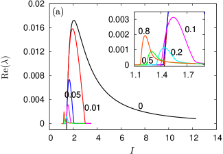
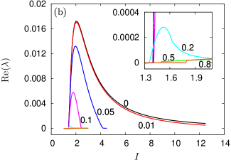
Figure 3: (Color online) Real part of the maximum eigenvalue $\lambda$ as a function of the dimensionless current $I$ for the different values (numbers on the panels) of $\mu$ (panel (a)) and $\zeta$ (panel (b)).

The asynchronous state is the steady state of the system (15):

$$Z_{0}(\eta,\xi)=\text{i}\frac{I-\sqrt{I^{2}-(1+\xi)^{2}}}{1+\xi},$$ (16)

$$Q_{0}=\omega_{0}^{-2}\iint\,d\eta\,d\xi\;W(\eta,\xi)\,(1+\eta)\sqrt{I^{2}-(1+\xi)^{2}}\;,$$

where we assume $\langle\xi\rangle=\langle\eta\rangle=0$. Remarkably, the disorder in the junction resistances (parameter $\eta$) does not influence the value $Z_{0}$, only the disorder in critical currents (parameter $\xi$). However, the stability of this asynchronous state depends on distributions of $\eta$ and $\xi$. We consider two cases, with a disorder in one parameter only.

(i) Disorder in resistances. Here we assume that $W(\eta,\xi)=\delta(\xi)W_{\mu}(\eta)$ where $W_{\mu}$ is a uniform distribution in the interval $(-\mu,\mu)$. To study the perturbations in the integral equation (15) at the steady solution (16), we discretized the integral using 500 nodes and found the eigenvalues of the resulting matrix. The results for the maximal eigenvalue are shown in Fig. 3a. One can see that, with increasing the external current $I$, the asynchronous state loses stability almost at the same critical value as for identical junctions (expression (11)), but for large values of $I$ the stability is restored. The region of instability decreases for larger disorder $\mu$.

(ii) Disorder in critical currents. Here we assume that $W(\eta,\xi)=\delta(\eta)W_{\zeta}(\xi)$, where $\zeta$ is the width of the uniform distribution. With the same procedure as in case (i) we found the stability eigenvalues that are shown in Fig. 3b. Qualitatively, the pictures look similar: both disorders result in a finite (in therms of the external current $I$) region of instability of the asynchronous state.

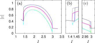
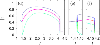
Figure 4: (Color online) Panels (a),(d): Dependence of the averaged order parameter $|z|$ on current $I$, $\mu=0.01,\,\zeta=0$ and $\mu=0,\,\zeta=0.05$ respectively. Three lines show the maximal (upper dashed line), the average (solid line), and the minimal (lower dashed line) value of variations of $|z|$ in time, in the asynchronous states these lines coincide. Panels (c), (d), (e) and (f) show enlargements of the regions near the synchrony-asynchrony transitions, to demonstrate the hysteresis.

Both calculations presented in Fig. 3 show, that the main effect of disorder in arrays is in the establishing of stability of the asynchronous state for large values of current $I$, while only in some range (which decreases with disorder) the asynchrony is unstable. We illustrate the appearing synchrony patterns in disordered arrays in the next subsection.

III.3 Numerical simulations

Dynamics of the nonhomogeneous arrays of Josephson junctions is illustrated in Figs. 4. As above, we consider not a general situation where both the critical current and the resistance are spread, but cases where one of these parameters has a distribution. In numerical simulations we use the discrete representation (14). In order to avoid spurious non-smooth solutions, an additional very small viscous term $\sim(Z_{k+1}+Z_{k-1}-2Z_{k})$ was added to the equation for $Z_{k}$ that ensures numerical stabilization of the integro-differential equation.

To characterize synchrony we calculated the average over the array order parameter $z=M^{-1}\sum_{k}Z_{k}$ and plot it vs. parameter $I$ in Fig. 4. In the asynchronous state this parameter attains the fixed point (cf. Eq. (16)), while in the synchronous state it oscillates arround some mean value (because of disorder the synchrony is not complete, so $|z|<1$). Remarkably, also in the case of disorder, the transition to synchrony demonstrates hysteresis both for small and large values of $I$, as can be seen on panels (b),(c),(e), and (f) of Fig. 4.

IV Conclusion

In this paper we applied the approach by Watanabe and Strogatz to the description of the synchronization transition in an array of Josephson junctions with an LCR load. For identical junctions a closed low-dimensional system of equations for global variables (the Watanabe-Strogatz variables for the junctions and two variables describing the load) demonstrates a region of bistability at the transition from asynchrony to full synchrony, so that this transition shows hysteresis. This confirms previous results based on the approximate self-consistent reduction to the Kuramoto model Heath and Wiesenfeld (2000). For nonidentical junction the method yields an integro-differential system, as each group of junctions having certain parameters is described by the WS variables. Here, with the growth of the variability of parameters, the region of synchronization shrinks. Transition to synchrony in this case is also hysteretic.

Validity of the WS approach to the Josephson junction array is based on the fact, that for standard junctions the dependence of the superconducting current on the phase is a simple sine function. Therefore, the theory is also valid for so-called $\pi$-junctions Buzdin (2005), where the current has an opposite direction but nevertheless is propotional to $\sin(\varphi)$. However, for recently constructed so-called $\varphi$-junctions Sickinger et al. (2012), where the phase dependence of the current contains the second harmonics, the WS approach is not applicable, and synchronization of such junctions remains a challenging problem.