Bifurcation diagram and stability for
a one-parameter family of planar vector fields

Abstract.

We consider the 1-parameter family of planar quintic systems, $\dot{x}=y^{3}-x^{3}$, $\dot{y}=-x+my^{5}$, introduced by A. Bacciotti in 1985. It is known that it has at most one limit cycle and that it can exist only when the parameter $m$ is in $(0.36,0.6)$. In this paper, using the Bendixon-Dulac theorem, we give a new unified proof of all the previous results, we shrink this to $(0.547,0.6)$, and we prove the hyperbolicity of the limit cycle. We also consider the question of the existence of polycycles. The main interest and difficulty for studying this family is that it is not a semi-complete family of rotated vector fields. When the system has a limit cycle, we also determine explicit lower bounds of the basin of attraction of the origin. Finally we answer an open question about the change of stability of the origin for an extension of the above systems.

1. Introduction and main results

A. Bacciotti, during a conference about the stability of analytic dynamical systems, held in Florence in 1985, proposed to study the stability of the origin of the following quintic system

$$\left\{\begin{array}[]{lll}\dot{x}=y^{3}-x^{3},\\ \dot{y}=-x+my^{5},\qquad m\in\mathbb{R}.\end{array}\right.$$ (1)

Two years later, a quite complete study of (1) was done by Galeotti and Gori in [10]. They prove that, when $m\in(-\infty,0.36]\cup[0.6,\infty)$, system (1) has no limit cycles and, otherwise, it has at most one. Their proofs are mainly based on the study of the stability of the limit cycles, controlled by the sign of its characteristic exponent, together with a transformation of the system using a special type of adapted polar coordinates. Their proof of the uniqueness of the limit cycle does not provide its hyperbolicity.

In this paper we refine the above results. To guess which is the actual bifurcation diagram we did first a numerical study, obtaining the following: it seems that there exists a value $m^{*}>0$, such that:

1. System (1) has no limit cycles if $m\in(-\infty,m^{*}]\cup[0.6,+\infty)$. Moreover, for $m=m^{*}$ it has a heteroclinic polycycle formed by the separatrices of the two saddle points located at $(\pm m^{-1/4},\pm m^{-1/4})$.

2. For $m\in(m^{*},0.6)$ the system has exactly one unstable limit cycle.

3. The value $m^{*}$ is approximately $0.560115.$

Recall that a polycycle is a simple closed curve formed by several solutions of the system and admitting a Poincaré return map. The first two items coincide with the ones described in [10]. In that paper it is claimed that $m^{*}$ is between $0.58$ and $0.59$, but our computations give a different result, which we believe that is the right one.

The first aim of this work is to obtain analytic results that confirm, as much as possible, the above description. To clarify the phase portraits of the system, we will draw them on the Poincaré disc, see [3, 24].

For $m\leq 0$, system (1) has no periodic orbits because $x^{2}/2+y^{4}/4$ is a global Lyapunov function. Therefore, the origin is a global attractor. In particular, its phase portrait is trivial. Therefore, we will concentrate on the case $m>0.$ In this case, the system has three critical points, $(\pm m^{-1/4},\pm m^{-1/4})$ and $(0,0)$. The first couple of points are saddles and the third one is a monodromic nilpotent singularity. Its stability can be determined using the tools introduced in [2, 19], see Subsection 2 and next Theorem 1.3. We prove:

Theorem 1.1.

Consider system (1).

• It has neither periodic orbits, nor polycycles, when $m\in(-\infty,0.547]\cup[0.6,\infty)$. Otherwise, it has at most one periodic orbit or one polycycle and both can not coexist. Moreover, when the limit cycle exists, it is hyperbolic and unstable.

• For $m>0,$ their phase portraits on the Poincaré disc, are given in Figure 1.

• Let $\mathcal{M}$ be the set of values of $m$ for which it has a heteroclinic polycycle. Then $\mathcal{M}$ is finite, non-empty and it is contained in $(0.547,0.6)$. Moreover, when $m\in{\mathcal{M}}$, the corresponding system has no limit cycles and its phase portrait is given by Figure 1 (b).

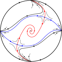
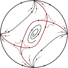
(a) When $m\in(0,0.547]$, or when	(b) When $m\in(0.547,0.6)$ and
$m\in(0.547,0.6)$ and neither the	the polycycle exists.
polycycle nor the limit cycle exist.
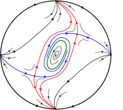
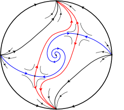
(c) When $m\in(0.547,0.6)$ and	(d) For $m\in[0.6,\infty)$
the limit cycle exists.

Figure 1. Phase portraits of system (1).

Our simulations show that (a), (b) and (c) of Figure 1 occur when $m\in(0,m^{*})$, $m=m^{*}$ and $m>m^{*}$, respectively, for some $m^{*}\in(0.547,0.6)$, that numerically we have found to be $m^{*}\approx 0.560115.$ We have not been able to prove the existence of this special value $m^{*},$ because our system is not a semi-complete family of rotated vector fields (SCFRVF) and this fact hinders the obtention of the full bifurcation diagram; see the discussion in Subsection 3.1 and Example 7.1. This is precisely the reason for which we have decided to push forward in the study of system (1). Our approach can be useful to understand other interesting polynomial systems of differential equations that have been considered previously; see for instance [4, 8].

In any case, from our result, we know the existence of finitely many values $m^{*}_{j},$ $j=1,\ldots,k,$ where $k\geq 1$, satisfying $0.547<m^{*}_{1}<m^{*}_{2}<\cdots m^{*}_{k}<0.6$, such that phase portrait (b) only happens for these values. Moreover, for $m\in(0.547,m^{*}_{1})$, phase portrait (a) holds, for $m\in(m^{*}_{k},0.6)$ phase portrait (c) holds, and for each one of the remainder $k-1$ intervals, the phase portrait does not vary on each interval and is either (a) or (c).

As a byproduct of our approach we can also give explicit algebraic restrictions on the initial conditions to ensure that the solutions starting at them tend to the origin.

Recall that when a critical point, $\mathbf{p}\in\mathbb{R}^{n}$, of a differential system is an attractor we can define its basin of attraction as

$$\mathcal{W}^{s}_{\mathbf{p}}=\{\mathbf{x}\in\mathbb{R}^{n}\,:\,\lim_{t\to+\infty}\varphi(t,\mathbf{x})=\mathbf{p}\},$$

where $\varphi$ denotes the solution of the differential system such that $\varphi(0,\mathbf{x})=\mathbf{x}.$ A very interesting question, mainly motivated by Control Theory problems, consists in obtaining testable conditions for ensuring that some initial condition is in $\mathcal{W}^{s}_{\mathbf{p}}.$ Usually these conditions are obtained using suitable Lyapunov functions. We prove next result using a different approach based on the construction of Dulac functions.

Proposition 1.2.

Let $\mathcal{W}^{s}_{\mathbf{0}}$ be the basin of attraction of the origin of system (1). Consider $V_{m}(x,y)=g_{0,m}(y)+g_{1,m}(y)x+g_{2,m}(y)x^{2}$, with

$$g_{2,m}(y)= \frac{1}{89100}(3-10m)(3+35m)y^{12}-\frac{1}{6300}(75-125m)^{2/3}(3-13m)y^{8}$$

$$+\frac{1}{90}(3-10m)y^{6}-\frac{1}{25}(75-125m)^{2/3}y^{2}+1,$$

$g_{1,m}(y)=g_{2,m}^{\prime}(y)$ and $g_{0,m}(y)=g_{2,m}^{\prime\prime}(y)/2-my^{5}g_{2,m}^{\prime}(y)/2+5my^{4}g_{2,m}(y)/3.$ Then, for $m\in(0.5,0.6),$ $\mathcal{U}_{m}\subset\mathcal{W}^{s}_{\mathbf{0}}$, where $\mathcal{U}_{m}$ is the bounded connected component of $\{(x,y)\in\mathbb{R}^{2}\,:\,V_{m}(x,y)\leq 0\},$ that contains the origin and whose boundary is the oval of $V_{m}(x,y)=0,$ see Figure 2.

Figure 2. The limit cycle of system (1) and the set $\mathcal{U}_{m}$, introduced in Proposition 1.2, when $m=0.57.$

As we will see, the proof of the above proposition is an straightforward consequence of Proposition 5.2. Using the same tools, it can be shown that the same result also holds for smaller values of $m$. In any case, notice that this proposition covers all the values of $m$ for which the system has limit cycles.

Studying the stability of the origin of system (1) we realized that, using the same tools, we could solve an open question left in [10]. Our third result studies the stability of the origin of the following generalization of system (1):

$$\left\{\begin{array}[]{lll}\dot{x}=y^{3}-x^{2k+1},\\ \dot{y}=-x+my^{2s+1},\qquad m\in\mathbb{R}\quad\mbox{and}\quad k,s\in\mathbb{N}^{+}.\end{array}\right.$$ (2)

In [10], the authors gave the stability of the origin when $s\neq 2k$ and ask whether it is true or not that the change of stability of the origin when $s=2k$ is at the value $m=(2k+1)/(4k+1)$. We will prove that their guess was not correct for $k>1$. Next result shows that when $s=2k$, the stability changes at

$$m=\frac{(2k+1)!!}{(4k+1)!!!!},$$ (3)

where, given $n\in\mathbb{N}^{+}$, $n!!$ and $n!!!!$ are defined recurrently, as follows,

$$n!!=n\times(n-2)!!,\quad n!!!!=n\times(n-4)!!!!,$$

with $1!!=1,2!!=2$ and $j!!!!=j$ for $1\leq j\leq 4.$ Notice that when $k=1,$ the right hand-side of (3) and $(2k+1)/(4k+1)$ coincide and give $m=3/5,$ which is one of the values appearing in Theorem 1.1.

Theorem 1.3.

Consider system (2). Then:

• When $s<2k$, the origin is an attractor when $m<0$ and a repeller when $m>0.$

• When $s>2k$, the origin is always an attractor.

• When $s=2k$, the origin is an attractor when $m<{(2k+1)!!}/{(4k+1)!!!!}$ and a repeller when the reverse inequality holds. Moreover, when $k=1$ and $m=3/5$ the origin is a repeller and for $m\lesssim 3/5$ system (1) has at least one limit cycle near the origin.

The method used to study the stability of the origin of (2), when $s=2k$ and $k=1$, also works for deciding its stability for the cases not covered by the above theorem: $s<2k$ and $m=0$; and $s=2k$, $k>1$ and $m$ as in (3). Nevertheless, the computations are tedious and we have decided do not perform them.

The paper is structured as follows. In Section 2 we prove Theorem 1.3. Section 3 collects some preliminary results. It starts with a discussion on the differences between being or not, a SCFRVF. Then, subsection 3.2 is devoted to study the singularities at infinite of system (1) and their phase portraits on the Poincaré disc. Afterwards, we present some Bendixson-Dulac type results that we will use to prove non-existence or uniqueness of periodic orbits or polycycles. Finally, we introduce a result for controlling the number of roots of 1-parameter families of polynomials and we show that our system can be reduced to an Abel differential equation.

In Section 4 we prove the non-existence results for $m\in(-\infty,0.36]\cup[0.6,\infty)$. Our proof is different of that of [10] and it is mainly based on the use of Dulac functions.

In Section 5 we prove the existence of at most one periodic orbit when $m\in(1/2,0.6)$. Our approach also gives the hyperbolicity of the orbit and again uses a Bendixson-Dulac type result. This section also includes the proof of Proposition 1.2.

Section 6 is devoted to enlarge the region where we can assure the non existence of periodic orbits and polycycles, proving this for $m\in(9/25,0.547]$. The proof uses once more a suitable Dulac function in a part of the interval and the Poincaré-Bendixon theorem, together with the hyperbolicity of the limit cycle, whenever it exists, for the remaining values of $m.$

Section 7 deals with the existence of polycycles for the system. Finally in Section 8 we glue all the above results to prove Theorem 1.1.

2. Stability of the origin and proof of Theorem 1.3

Notice that the origin of (1) and (2) are nilpotent critical points and there are several tools for studying its local stability, see for instance [2, 15, 19]. We will follow the approach of [2, 15], based on the polar coordinates introduced by Lyapunov in [17], to study of the stability of degenerate critical points.

Let $u(\varphi)=\operatorname{Cs}(\varphi)$ and $v(\varphi)=\operatorname{Sn}(\varphi)$ be the solutions of the Cauchy problem:

$$\dot{u}=-v^{2p-1},\,\dot{v}=u^{2q-1},\quad u(0)=\root 2q \of{1/p}\quad\mbox{ and }\quad v(0)=0,$$

where the prime denotes the derivative with respect to $\varphi$.

The Lyapunov generalized polar coordinates are $x=r^{p}\operatorname{Cs}(\varphi)$ and $y=r^{q}\operatorname{Sn}(\varphi)$. They parameterize the algebraic curves $px^{2q}+qy^{2p}=r^{2pq},$ that correspond to the level sets of above $(p,q)-$quasi-homogeneous Hamiltonian system. In particular, $p\operatorname{Cs}^{2q}(\varphi)+q\operatorname{Sn}^{2p}(\varphi)=1$, and both functions are smooth $T_{p,q}$-periodic functions, where

$$T=T_{p,q}=2p^{-1/2q}q^{-1/2p}\frac{\Gamma\left(\frac{1}{2p}\right)\Gamma\left(\frac{1}{2q}\right)}{\Gamma\left(\frac{1}{2p}+\frac{1}{2q}\right)},$$

and $\Gamma$ denotes the Gamma function. The general expression of a differential system in these coordinates is:

$$\dot{r}=\frac{x^{2q-1}\dot{x}+y^{2p-1}\dot{y}}{r^{2pq-1}},\quad\dot{\theta}=\frac{px\dot{y}-qy\dot{x}}{r^{p+q}}.$$ (4)

In the nilpotent monodromic case, the component $\dot{\theta}$ does not vanish in a punctured neighborhood of the critical point. Hence, system (4) can be written in a neighborhood of $r=0$ as

$$\frac{dr}{d\theta}=\sum_{i=1}^{\infty}R_{i}(\theta)r^{i},$$ (5)

where $R_{i}(\theta)$, $i\geq 1$ are $T$-periodic functions. The solution of (5) that for $\theta=0$ passes for $r=\rho$ can be written as the power series

$$r(\theta,\rho)=\rho+\sum_{i=2}^{\infty}u_{i}(\theta)\rho^{i},\quad\mbox{with}\quad u_{i}(0)=0,$$ (6)

and the functions $u_{i}$ can be computed solving recursive linear differential equations obtained plugging (6) in (5). It is well-known that the stability of the origin is given by the first non-vanishing generalized Lyapunov constant $V_{k}:=u_{k}(T)$.

To effectively compute some integrals of the above generalized trigonometric functions we will use the following result, see [15].

Lemma 2.1.

Let $\operatorname{Sn}$ and $\operatorname{Cs}$ be the (1,q)-trigonometrical functions and let $T$ be their period. Then, for $i,j\in\mathbb{N}$,

• $\int_{0}^{T}\operatorname{Sn}^{i}(\theta)\operatorname{Cs}^{j}(\theta)\,d\theta=0$ when either $i$ or $j$ are odd.

• $\int_{0}^{T}\operatorname{Sn}^{i}(\theta)\operatorname{Cs}^{j}(\theta)\,d\theta=\dfrac{2\Gamma\left(\frac{i+1}{2}\right)\Gamma\left(\frac{j+1}{2q}\right)}{q^{\frac{i+1}{2}}\Gamma\left(\frac{i+1}{2}+\frac{j+1}{2q}\right)}$ when $i$ and $j$ are both even.

• For $q=2,$ $\int_{0}^{\theta}\operatorname{Cs}^{8}(\psi)\,d\psi=\dfrac{6\operatorname{Sn}(\theta)\operatorname{Cs}^{5}(\theta)+10\operatorname{Sn}(\theta)\operatorname{Cs}(\theta)+5\theta}{21}.$

• For $q=2$, $\int_{0}^{\theta}\operatorname{Sn}^{4}(\psi)\,d\psi=\dfrac{-\operatorname{Sn}^{3}(\theta)\operatorname{Cs}(\theta)-\operatorname{Sn}(\theta)\operatorname{Cs}(\theta)+\theta}{7}.$

Proof of Theorem 1.3.

By using the transformation $(x,y)\to(y,x)$, system (2) becomes

$$\left\{\begin{array}[]{lll}\dot{x}=-y+mx^{2s+1},\\ \dot{y}=x^{3}-y^{2k+1}.\end{array}\right.$$ (7)

We use (4), with $p=1$ and $q=2$, to transform it into

$$\left\{\begin{array}[]{lll}\dot{r}=m\operatorname{Cs}^{2s+4}(\theta)r^{2s+1}-\operatorname{Sn}^{2k+2}(\theta)r^{4k+1},\\ \dot{\theta}=r-\operatorname{Cs}(\theta)\operatorname{Sn}^{2k+1}(\theta)r^{4k}-2m\operatorname{Cs}^{2s+1}(\theta)\operatorname{Sn}(\theta)r^{2s},\end{array}\right.$$

or equivalently,

$$\frac{dr}{d\theta}=\frac{m\operatorname{Cs}^{2s+4}(\theta)r^{2s}-\operatorname{Sn}^{2k+2}(\theta)r^{4k}}{1-\operatorname{Cs}(\theta)\operatorname{Sn}^{2k+1}(\theta)r^{4k-1}-2m\operatorname{Cs}^{2s+1}(\theta)\operatorname{Sn}(\theta)r^{2s-1}}.$$ (8)

The Taylor series of the right hand-side of (8) at the origin has three possibilities:

(i) When $s<2k$, then (8) becomes

$$\frac{dr}{d\theta}=m\operatorname{Cs}^{2s+4}(\theta)r^{2s}+O(r^{4k}).$$

Therefore, using the method explained above and Lemma 2.1, we get that its first Lyapunov constant is

$$V_{2s}=m\int_{0}^{T}\operatorname{Cs}^{2s+4}(\theta)\,d\theta=\frac{m\,\sqrt{2\pi}\,\Gamma\left(\frac{2s+5}{4}\right)}{\Gamma\left(\frac{2s+7}{4}\right)}.$$ (9)

Then $m=0$ is the bifurcation value, and the origin of (2) changes its stability from attractor to repeller as $m$ goes from negative values to positive values.

(ii) Suppose $s>2k$, then the Taylor expansion of (8) at $r=0$ is

$$\frac{dr}{d\theta}=-\operatorname{Sn}^{2k+2}(\theta)r^{4k}+O(r^{2s}).$$

By using the same method, we obtain that the first Lyapunov constant is

$$V_{4k}=\int_{0}^{T}-\operatorname{Sn}^{2k+2}(\theta)\,d\theta=-\frac{\Gamma\left(\frac{1}{4}\right)\Gamma\left(\frac{2k+3}{2}\right)}{2^{\frac{2k+1}{2}}\Gamma\left(\frac{4k+7}{4}\right)}<0,$$ (10)

and the stability of the origin of (2) is independent of $m$ and it is an attractor for all $m$.

(iii) Finally, when $s=2k$ we have

$$\frac{dr}{d\theta}=\left(m\operatorname{Cs}^{4k+4}(\theta)-\operatorname{Sn}^{2k+2}(\theta)\right)r^{4k}+O(r^{8k-1}).$$ (11)

Hence the first non-vanishing generalized Lyapunov constant is given by

$$V_{4k}=\int_{0}^{T}\left(m\operatorname{Cs}^{4k+4}(\theta)-\operatorname{Sn}^{2k+2}(\theta)\right)d\theta.$$

By using (9) with $s=2k$ and (10), after some simplifications, we obtain that

$$V_{4k}=\frac{2\pi^{3/2}\big{(}m(4k+1)!!!!-(2k+1)!!\big{)}}{\left(\Gamma\left(\frac{3}{4}\right)\right)^{2}(4k+3)!!!!}.$$

Therefore the origin of (2) is attractor for $m<(2k+1)!!/(4k+1)!!!!$ and repeller for $m>(2k+1)!!/(4k+1)!!!!$, as we wanted to prove.

In the particular case $s=2k$ and $k=1$, that corresponds to system (1), and when $m=3/5$ we have that $V_{4}=0.$ To proof the theorem we continue computing the next non-zero Lyapunov constant. For $s=2$ and $k=1$, equation (8) writes as

$$\frac{dr}{d\theta}=R_{4}(\theta)r^{4}+R_{7}(\theta)r^{7}+R_{10}(\theta)r^{10}+O(r^{13}),$$

with $R_{4}(\theta)=m\operatorname{Cs}^{8}(\theta)-\operatorname{Sn}^{4}(\theta)$,

$$R_{7}(\theta)=2m^{2}\operatorname{Cs}^{13}(\theta)\operatorname{Sn}(\theta)+m\operatorname{Cs}^{9}(\theta)\operatorname{Sn}^{3}(\theta)-2m\operatorname{Cs}^{5}(\theta)\operatorname{Sn}^{5}(\theta)-\operatorname{Cs}(\theta)\operatorname{Sn}^{7}(\theta)$$

and

$$R_{10}(\theta)= 4m^{3}\operatorname{Cs}^{18}(\theta)\operatorname{Sn}^{2}(\theta)+4m^{2}\operatorname{Cs}^{14}(\theta)\operatorname{Sn}^{4}(\theta)+m(1-4m)\operatorname{Cs}^{10}(\theta)\operatorname{Sn}^{6}(\theta)$$

$$-4m\operatorname{Cs}^{6}(\theta)\operatorname{Sn}^{8}(\theta)-\operatorname{Cs}^{2}(\theta)\operatorname{Sn}^{10}(\theta),$$

with $m=3/5$. Following the procedure explained in this section we obtain that $u_{2}=u_{3}=0$,

$$u_{4}(\theta) =\int_{0}^{\theta}R_{4}(\psi)\,d\psi,\quad u_{5}=u_{6}=0,$$

$$u_{7}(\theta) =\int_{0}^{\theta}\big{(}R_{7}(\psi)+4R_{4}(\psi)u_{4}(\psi)\big{)}\,d\psi,\quad u_{8}=u_{9}=0,$$

$$u_{10}(\theta) =\int_{0}^{\theta}\Big{(}R_{10}(\psi)+7R_{7}(\psi)u_{4}(\psi)+4R_{4}(\psi)u_{7}(\psi)+6R_{4}(\psi)u_{4}^{2}(\psi)\Big{)}\,d\psi.$$

Using Lemma 2.1 and some easy computations we get that $V_{1}=\cdots=V_{9}=0$. Finally, it suffices to compute

$$V_{10}=\int_{0}^{T}\Big{(}R_{10}(\theta)+7R_{7}(\theta)u_{4}(\theta)+4R_{4}(\theta)u_{7}(\theta)\Big{)}\,d\theta,$$

because $\dfrac{du_{4}^{3}(\theta)}{d\theta}=3R_{4}(\theta)u_{4}^{2}(\theta).$ Using integration by parts and the expression of $u_{7}^{\prime}$ we arrive to

$$V_{10}=\int_{0}^{T}\Big{(}R_{10}(\theta)+3u_{4}(\theta)u_{7}^{\prime}(\theta)\Big{)}\,d\theta=\int_{0}^{T}\Big{(}R_{10}(\theta)+3u_{4}(\theta)R_{7}(\theta)\Big{)}\,d\theta.$$ (12)

Notice that applying (iii) and (iv) of Lemma 2.1 we know that

$$u_{4}(\theta)=\int_{0}^{\theta}\Big{(}\frac{3}{5}\operatorname{Cs}^{8}(\psi)-\operatorname{Sn}^{4}(\psi)\Big{)}\,d\psi=\frac{6\operatorname{Sn}(\theta)\operatorname{Cs}^{5}(\theta)+15\operatorname{Sn}(\theta)\operatorname{Cs}(\theta)+5\operatorname{Sn}^{3}(\theta)\operatorname{Cs}(\theta)}{35}.$$

Plugging this expression in (12), using several times (i) and (ii) of Lemma 2.1 and the properties of the $\Gamma$ function we arrive to

$$V_{10}=\frac{128}{1625}\frac{\left(\Gamma\left(\frac{3}{4}\right)\right)^{2}}{\sqrt{\pi}}>0.$$

Hence the origin is unstable for $m=3/5$. As a consequence, we know that at $m=3/5$ the system has a Hopf-like bifurcation. Therefore the system has at least one limit cycle near the origin for $m\lesssim 3/5$. ∎

3. More preliminary results

This section is a miscellaneous one and it is divided into several short subsections containing either some tools that we will use to prove Theorems 1.1 and 1.2 or some preliminary results.

3.1. Differences between families that are SCFRVF and families that are not

On the one hand, if a one-parameter family of differential systems is a SCFRVF, then there are many results that allow to control the possible bifurcations; see [9, 22, 23]. One of the most useful ones is the so called non-intersection property. It asserts that if $\gamma_{1}$ and $\gamma_{2}$ are limit cycles corresponding to systems with different values of $m,$ then $\gamma_{1}\cap\gamma_{2}=\emptyset.$ Informally, we like to call this property Atila’s property because it implies that, if for some value of $m$ a limit cycle passes trough a region of the phase plane, this region turns out to be forbidden for the periodic orbits that the system could have for any other value of the parameter. As a consequence, in this case, the study of 1-parameter bifurcation diagrams is much simpler.

For instance, consider a 1-parameter SCFRVF satisfying the following property:

(P) For each $m\in(m_{0},m_{1})$, it has at most one limit cycle, that we denote by $\gamma_{m}$. Here, if for some $m$ the corresponding system has no limit cycles then $\gamma_{m}=\emptyset$. Moreover, assume that $\cup_{m\in(m_{0},m_{1})}\gamma_{m}$ covers a region of the plane where all the periodic orbits of the system have to cut.

Therefore, it holds that: for $m\in\mathbb{R}\setminus(m_{0},m_{1})$ the system has no periodic orbits.

The above property has very important practical consequences if we want to determine the values $m_{0}$ and $m_{1}$, that constitute, in many cases, the most difficult ones to be obtained to complete the bifurcation diagram. Usually, one of the values, say $m_{0}$ corresponds to a Hopf-like bifurcation, and some local analysis allows to obtain it. Then, for instance, if for some value of $m$, say $\widetilde{m}>m_{0}$, the system has no limit cycles then $m_{1}<\widetilde{m}$. The same idea can also be applied to obtain lower bounds of $m_{1}$. These facts simplify a lot the obtention of analytic bounds for the value $m_{1}$ because it suffices to deal with concrete systems, with fixed values of $m$. This approach has been applied with success in many works; see for instance [11, 14, 21, 23, 25].

On the other hand, if for a general family of vector fields, we have that the same property (P) given above holds, we can say nothing of what happens for $m\in\mathbb{R}\setminus(m_{0},m_{1})$. For this reason, when we study system (1), we can not ensure the existence of a unique value of $m$ for which phase portrait (b) of Figure 1 appears; see also Example 7.1. We remark that system (1) is not a SCFRVF with respect to $m$, and moreover we have not been able to transform it into an equivalent one that were a SCFRVF.

From our point of view, to introduce tools for studying 1-parameter families that are not SCFRVF is a challenge for the differential equations community.

3.2. Global phase portrait

We will draw the phase portraits of system (1) on the Poincaré disc, [3, 24]. Recall that, from the works of Markus [18] and Newmann [20], for knowing a phase portrait it suffices to determine the type of critical points (finite and at infinity), the configuration of their separatrices, and the number and character of their periodic orbits.

We start making a study of the critical points at infinity of the Poincaré compactification of the system. That is, we will use the transformations $(x,y)=(1/z,u/z)$ and $(x,y)=(v/z,1/z)$, with a suitable change of time to transform system (1) into two new polynomial systems, one in the $(u,z)$-plane and another one in the $(v,z)$-plane respectively; see [3] for the details. Then, for understanding the behavior of the solutions of (1) near infinity it suffices to study the type of critical points of the transformed systems which are localized on the line $z=0$. These points are precisely the so called critical points at infinity of system (1).

Lemma 3.1.

By using the transformation $(x,y)=\left(v/z,1/z\right)$ and the change of time $dt/d{\tau}=1/{z^{4}}$ system (1) is transformed into the system

$$\left\{\begin{array}[]{l}v^{\prime}=-mv+(1-v^{3})z^{2}+v^{2}z^{4},\\ z^{\prime}=-mz+vz^{5},\end{array}\right.$$ (13)

where the prime denotes the derivative with respect to $\tau$. The origin is the unique critical point of (13) on $z=0$ and it is an attracting node.

The proof of the above result is straightforward.

Lemma 3.2.

By using the transformation $(x,y)=\left(1/z,u/z\right)$ and the change of time $dt/d{\tau}=1/{z^{4}}$ system (1) is transformed into the system

$$\left\{\begin{array}[]{l}u^{\prime}=(u-z^{2})z^{2}+u^{4}(mu-z^{2}),\\ z^{\prime}=(1-u^{3})z^{3},\end{array}\right.$$ (14)

where the prime denotes the derivative with respect to $\tau$. The origin is the unique critical point of (14) on $z=0$ and it is a repeller.

Proof.

From the expression of (14) it is clear that the origin is its unique critical point on $z=0$. For determining its nature we will use the directional blow-up since the linear part of the system at this point vanishes identically; see again [3].

We apply the $z$-directional blow-up given by the transformation $r={u}/{z}$, $z=z$. Performing it, together with the change of time $dt/d\tau={z^{3}}$, system (14) is transformed into

$$\left\{\begin{array}[]{l}\dot{r}=-1+mzr^{5},\\ \dot{z}=1-z^{3}r^{3}.\end{array}\right.$$ (15)

System (15) has no critical points on $z=0$. Then by using the transformation $(u,z)=(rz,z)$ we can obtain the phase portrait of system (15). Recall that the mapping swaps the third and fourth quadrants in the $z$-directional blow-up. In addition, taking into account the change of time $dt/d\tau=z^{3}$, it follows that the vector field in the third and fourth quadrant of the plane $(u,z)$ has the opposite direction to the one obtained in the $(r,z)$-plane.

Next, we need to perform the $u$-directional blow-up for knowing the phase portrait in such direction. After that, by joining the information about the blow-ups in both directions, we will have the phase portrait of system (14).

The $u$-directional blow-up is given by the transformation $u=u$, $q={z}/{u}$, and with the change of time $dt/d\tau={u^{3}}$, system (14) is transformed into

$$\left\{\begin{array}[]{l}\dot{u}=-q^{2}(uq^{2}-1)-u^{2}(uq^{2}-m),\\ \dot{q}=q^{5}-muq.\end{array}\right.$$ (16)

On $q=0$, the origin is the unique critical point of the system, and since the linear part of the system at this point vanishes identically we have to use again some directional blow-ups.

Since the lower degree term of $\dot{q}u-\dot{u}q$ is $-q(2mu^{2}+q^{2})$, and it only vanishes on the direction $q=0$, to study the origin of system (16) it suffices to consider the $u$-directional blow-up. It is given by the transformation $u=u$, $s={q}/{u}$. Doing the change of time $dt/d\tau={u},$ system (16) becomes

$$\left\{\begin{array}[]{l}\dot{u}=-us^{2}(u^{3}s^{2}-1)-u(u^{3}s^{2}-m),\\ \dot{s}=s^{3}(u^{3}-1)+2s(u^{3}s^{4}-m).\end{array}\right.$$ (17)

For $s=0$, system (17) has a unique critical point at the origin. The linearization matrix at the origin has eigenvalues $m$ and $-2m$. Thus the origin of system (17) is a saddle.

Then by using the transformation $(u,q)=(u,su)$ we can obtain the phase portrait of system (16). Recall that the mapping swaps the second and the third quadrants in the $u$-directional blow-up. In addition, taking into account the change of time $dt/d\tau=u$ it follows that the vector field in the second and third quadrants of the plane $(u,q)$ has the opposite direction to the one in the $(u,s)$-plane. Once we have the phase portrait in the $(u,q)$-plane, we apply the transformation $(u,z)=(u,qu)$.

By considering the properties of the blow-up technic and from the analysis of all the intermediate phase portraits we obtain that the origin of system (14) is a repeller. ∎

Recall that the finite critical points are two hyperbolic saddles at $(\pm m^{-1/4},\pm m^{-1/4})$ and a monodromic nilpotent singularity $(0,0)$, whose stability is given in Theorem 1.3. Finally notice that the vector field is symmetric with respect to the origin. By joining to these properties all the information concerning the infinite critical points and using the existence and uniqueness results on the number of limit cycles and polycycles given in Theorem 1.1, we obtain the global phase portraits of system (1) given in Figure 1.

3.3. Some Bendixson-Dulac type criteria

Next statement is a Bendixson-Dulac type result, that mixes the Bendixson-Dulac Test given in the classical book [3, Thm. 31] and the one given in [12, Prop. 2.2]. It is adapted to our interests. Similar results appear in [5, 13, 16, 26].

Proposition 3.3 (Bendixson-Dulac Criterion).

Let $X=(P,Q)$ be the vector field associated to the $C^{1}$-differential system

$$\left\{\begin{array}[]{lll}\dot{x}=P(x,y),\\ \dot{y}=Q(x,y),\end{array}\right.$$ (18)

and let $\mathcal{U}\subset\mathbb{R}^{2}$ be an open region with boundary formed by finitely many algebraic curves. Assume that there exists a rational function $V(x,y)$ and $k\in\mathbb{R}^{+}$ such that

$$M=M_{\{V,k\}}(x,y)=\langle\nabla V,X\rangle-kV\operatorname{div}(X)$$ (19)

does not change sign in $\mathcal{U}$ and $M$ only vanishes on points, or curves that are not invariant by the flow of $X$. Then,

• If all the connected components of $\mathcal{U}\setminus\{V=0\}$ are simple connected then the system has neither periodic orbits nor polycycles.

• If all the connected components of $\mathcal{U}\setminus\{V=0\}$ are simple connected, except one, say  $\widetilde{\mathcal{U}}$, that is 1-connected, then, either the system has neither periodic orbits nor polycycles or it has at most one of them in $\mathcal{U}$. Moreover, when it has a limit cycle, it is hyperbolic, is contained in $\widetilde{\mathcal{U}}$, and its stability is given by the sign of $-VM$ on  $\widetilde{\mathcal{U}}$.

Proof.

Consider the Dulac function $g(x,y)=|V(x,y)|^{-1/k}$. Then

$$\operatorname{div}(gX) =\frac{\partial g}{\partial x}P+\frac{\partial g}{\partial y}Q+g(\frac{\partial P}{\partial x}+\frac{\partial Q}{\partial y})=\langle\nabla g,X\rangle+g\operatorname{div}(X)$$

$$=-\frac{1}{k}\operatorname{sign}(V)|V|^{-\frac{k+1}{k}}\left(\langle\nabla V,X\rangle-kV\operatorname{div}(X)\right)$$

$$=-\frac{1}{k}\operatorname{sign}(V)|V|^{-\frac{k+1}{k}}M_{\{V,k\}}=-\frac{1}{k}\operatorname{sign}(V)|V|^{-\frac{k+1}{k}}M.$$

By the hypotheses, $M|_{\{V=0\}}=\langle\nabla V,X\rangle|_{\{V=0\}}$ does not change sign in $\mathcal{U}$ and there is no solution contained in $\{M=0\}.$ Therefore, neither the periodic orbits nor the polycycles of the vector field in $\mathcal{U}$ can intersect $\{V=0\}.$

For proving (I) we follow the proof of the Bendixson-Dulac Criterion given in [3, Thm. 31]. Assume, to arrive a contradiction, that the system has a simple closed curve $\Gamma$ which is union of trajectories of the vector field. Let $C\subset\mathcal{U}$ the bounded region with boundary $\Gamma.$ Then, by Stokes Theorem, we have that

$$\iint_{C}\operatorname{div}(gX)=\int_{\Gamma}\langle gX,\mathbb{n}\rangle,$$

where $\Gamma$ is oriented in the suitable way. Note that the right hand-side term in this equality is zero because $gX$ is tangent to the curve $\Gamma$ and the left one is non-zero by our hypothesis. This fact leads to the desired contradiction.

In case (II), applying a similar argument to the region bounded by two possible simple closed curves formed by trajectories of the vector field, we arrive again to a contradiction.

To end the proof, let us show the hyperbolicity of the possible limit cycle $\Gamma$. Write $\Gamma=\{\gamma(t):=(x(t),y(t)),t\in[0,T]\}\subset\widetilde{U},$ where $T$ is its period, and its characteristic exponent as $h(\Gamma)=\int_{0}^{T}\operatorname{div}\left(X(\gamma(t))\right)\,dt.$ We need to prove that $h(\Gamma)\neq 0$ and that its sign coincides with the sign of $-VM$ on $\widetilde{U}.$ We know that

$$\frac{M}{V}=\frac{\langle\nabla V,X\rangle}{V}-k\operatorname{div}(X).$$

Remember that $\Gamma\cap\{V=0\}=\emptyset.$ Evaluating this last equality on $\gamma$ and integrating between 0 and $T$ we obtain that

$$\int_{0}^{T}\frac{M}{V}(\gamma(t))\,dt= \int_{0}^{T}\frac{\langle\nabla V,X\rangle}{V}(\gamma(t))\,dt-k\int_{0}^{T}\operatorname{div}(X)(\gamma(t))\,dt$$

$$= \ln|V(\gamma(t))|\Big{|}_{t=0}^{t=T}-k\,h(\Gamma)=-k\,h(\Gamma).$$ (20)

Therefore, the result follows. ∎

Next result is an straightforward consequence of the above proposition. It notices that when we construct a suitable Dulac function, the same method provides an effective estimation of the basin of attraction of the attracting critical points.

Corollary 3.4.

Assume that we are under the hypotheses of the above theorem and moreover that $\{V(x,y)=0\}$ has an oval such that it and the bounded region surrounded by it, say $\mathcal{W}$, are contained in $\mathcal{U}$. Then, if the differential system has only a critical point ${\bf p}$ in $\mathcal{W}$, and it is an attractor, then $\mathcal{W}$ is contained in the basin of attraction of $\bf p$.

Observe that when we are under the hypotheses of the above corollary, but we already know that the system has a limit cycle in $\mathcal{U}$, and $\mathcal{U}$ is simply connected, then, unless the set $\{V(x,y)=0\}$ reduces to a single point, there is no need to assume that $\{V(x,y)=0\}$ has an oval. The existence of the oval is already guaranteed by the method itself.

Sometimes the hypothesis that $M$ does not change sign can be replaced for another one, following next remark.

Remark 3.5.

Assume that in Proposition 3.3 we can not ensure that the function $M$, given in (19), keeps sign on the whole domain $\mathcal{U}$. Then, this hypothesis can be changed by another one. Define $\{M=0\}^{*}$ to be the subset of $\{M=0\}$ formed by curves that separate the regions $\{M>0\}$ and $\{M<0\}$. Then, the new hypothesis is that the set $\{M=0\}^{*}$ is without contact by the flow of $X$. Then, in the conclusions of the proposition, the connected components of $\mathcal{U}\setminus\{V=0\}$ must be replaced by the connected components of $\mathcal{U}\setminus\big{(}\{V=0\}\cup\{M=0\}^{*}\big{)}$ and the same type of conclusions hold. We will use this idea in the proof of Proposition 6.1.

3.4. Zeros of 1-parameter families of polynomials

As usual, for a polynomial $P(x)=a_{n}x^{n}+\cdots+a_{1}x+a_{0},$ we write $\triangle_{x}(P)$ to denote its discriminant, that is,

$$\triangle_{x}(P)=(-1)^{\frac{n(n-1)}{2}}\frac{1}{a_{n}}\operatorname{Res}(P(x),P^{\prime}(x)),$$

where $\operatorname{Res}(P,P^{\prime},x)$ is the resultant of $P$ and $P^{\prime}$ with respect to $x$; see [7].

By using the same techniques that in [11, Lem. 8.1], it is not difficult to prove the following result that will be used in several parts of the paper.

Lemma 3.6.

Let $G_{m}(x)=g_{n}(m)x^{n}+g_{n-1}(m)x^{n-1}+\cdots+g_{1}(m)x+g_{0}(m)$ be a family of real polynomials depending continuously on a real parameter $m$ and set $\Lambda_{m}=(c(m),d(m))$ for some continuous functions $c(m)$ and $d(m)$. Suppose that there exists an interval $I\subset\mathbb{R}$ such that:

• For some $m_{0}\in I$, $G_{m_{0}}$ has exactly $r$ zeros in $\Lambda_{m_{0}}$ and all them are simple.

• For all $m\in I$, $G_{m}(c(m))\cdot G_{m}(d(m))\neq 0$.

• For all $m\in I,$ $\triangle_{x}(G_{m})\neq 0.$

Then for all $m\in I$, $G_{m}(x)$ has also exactly $r$ zeros in $\Lambda_{m}$ and all them are simple.

The idea of the proof consists in looking at the roots of $G$ as continuous functions of $m$. The hypothesis (ii) prevents that some real roots of $G_{m}$ passes, varying $m$, trough the boundary of $\Lambda_{m}$. The hypothesis (iii) forbids, that varying $m$, appears some multiple root of $G_{m}$.

Notice that the above result transforms the control of the zeros of a function depending on two variables, $x$ and $m$, into three problems of only one variable, the one of item (i) with the variable $x$ and the two remainder ones with the variable $m$. If the dependence on $m$ is also polynomial, and the polynomial has rational coefficients, then these three simpler questions can be solved by applying the well-known Sturm method. As we will see in the proof of Proposition 5.2, this approach can also extended when the one variable polynomial has some irrational coefficients.

3.5. Transformation into an Abel equation

System (1) can be seen as the sum of two quasi-homogeneous vector fields, see [6]. It is known that in many cases these systems can be transformed into Abel equations. We get:

Proposition 3.7.

The periodic orbits of system (1) correspond to positive $T$-periodic solutions of the Abel equation

$$\frac{d\rho}{d\theta}=\alpha(\theta)\rho^{3}+\beta(\theta)\rho^{2},$$ (21)

where

$$\alpha(\theta)=3\operatorname{Cs}(\theta)\operatorname{Sn}(\theta)\left(2m\operatorname{Cs}^{4}(\theta)+\operatorname{Sn}^{2}(\theta)\right)\left(m\operatorname{Cs}^{8}(\theta)-\operatorname{Sn}^{4}(\theta)\right)$$

and

$$\beta(\theta)=5m\operatorname{Cs}^{8}(\theta)-4\operatorname{Sn}^{4}(\theta)+(3-10m)\operatorname{Cs}^{4}(\theta)\operatorname{Sn}^{2}(\theta),$$

being $\operatorname{Sn}$ and $\operatorname{Cs}$ the functions introduced in Subsection 2 and $T$ their period.

Proof.

The result follows by applying the Cherkas transformation

$$\rho=\frac{r^{3}}{1-r^{3}\operatorname{Sn}(\theta)\operatorname{Cs}(\theta)\left(\operatorname{Sn}^{2}(\theta)+2m\operatorname{Cs}^{4}(\theta)\right)},$$

to the expression of system (1) in the quasi-homogeneous polar coordinates introduced in Section 2. It is used that the periodic orbits of the system do not intersect the curve $\dot{\theta}=0$, and therefore the above transformation is well-defined over them, see [6]. ∎

Using the above expression it is not difficult to reproduce the proof of the existence of the Hopf-like bifurcation given in Subsection 2. Unfortunately, although expression (21) looks quite simple, the results about the number of limit cycles of Abel equations that we know are not applicable to (21).

4. Non-existence of limit cycles for $m\in(0,9/25)\cup(3/5,\infty)$

In this section we prove the non-existence results of periodic orbits already given in [10] and extend them to the non-existence of polycycles. Our proof is different and based on the Bendixson-Dulac theorem and other classical tools. We study separately each interval.

Proposition 4.1.

For $m\in(0,9/25]$, system (1) has neither periodic orbits nor polycycles.

Proof.

Recall that for $m\in(0,9/25]$ the origin is attractor. Therefore if we prove that any periodic orbit $\Gamma$ of the system is also attractor we will have proved that the system has not periodic orbits. In order to prove the stability of the limit cycle we need to compute $\int_{0}^{T}\operatorname{div}\left(X(\gamma(t))\right)\,dt$, where $\gamma(t):=(x(t),y(t))$ is the time parametrization of $\Gamma$, and $T=T(\Gamma)$ its period.

From equation (19), for any function $V$ such that $\{V(x,y)=0\}\cap\Gamma=\emptyset$, we have

$$\operatorname{div}(X)=\frac{M_{\{V,k\}}-\langle\nabla V,X\rangle}{-kV}.$$

Hence,

$$\int_{0}^{T}\operatorname{div}\left(X(\gamma(t))\right)\,dt=-\int_{0}^{T}\frac{M_{\{V,k\}}(\gamma(t))}{kV(\gamma(t))}dt,$$

where we have followed similar computations that in (3.3). Then the stability of $\Gamma$ is given by the sign of $-MV$. If we show that for $m\in(0,9/25]$ there exist a non-negative $V$ and $k\in\mathbb{R}^{+}$, such that its corresponding $M$ is non-negative, then we will have proven that the limit cycle is hyperbolic and attractor.

By considering $V(x,y)=2x^{2}+y^{4}$ and $k=2/3$ equation (19) becomes

$$M_{\{V,\frac{2}{3}\}}=\frac{2}{3}\left((3-10m)x^{2}+my^{4}\right)y^{4},$$

which clearly is non-negative on $\mathbb{R}^{2}$ for $m\in(0,3/10]$.

If we use the same $V(x,y)$ that in previous case, but $k=K(m)=8(11m+R)/(10m+3)^{2}$, with $R=\sqrt{m(1-4m)(25m-9)}$ then we have

$$M_{\{V,K(m)\}}=\left(\frac{2}{3+10m}\left(\frac{(m+R)(11m+R)}{m}\right)^{1/2}x^{2}+\frac{2(3-10m)}{3+10m}\left(\frac{m(11m+R)}{(m+R)}\right)^{1/2}y^{4}\right)^{2},$$

hence $M_{\{V,K(m)\}}$ is non-negative on $\mathbb{R}^{2}$ for $m\in(1/4,9/25]$.

Therefore system (1) has no limit cycles for $m\in(0,9/25]$ as we wanted to show.

To prove the non-existence of polycycles for $m\in(0,9/25)$ we use a different approach. Following [24], we can associate to each polycycle $\Gamma$, with $k$ hyperbolic saddles at its corners, the number $\rho(\Gamma)=\prod_{i=1}^{k}{b_{i}}/{a_{i}},$ where $-a_{i}<0<b_{i},$ $i=1,\ldots k,$ are the eigenvalues at the saddles. Then, $\Gamma$ is stable (respectively, unstable) if $\rho(\Gamma)<1$ (respectively, $\rho(\Gamma)>1$). In our case

$$\rho(\Gamma)=\frac{\left(5\sqrt{m}-3+\sqrt{25m+18\sqrt{m}+9}\right)^{4}}{48^{2}{m}}.$$

Then, easy computations show that the polycycle is an attractor if $m<9/25$ and a repeller if $m>9/25$. Assume, to arrive to a contradiction, that for $m<9/25$ the polycycle exists. Then both, the polycycle and the origin, would be attractors. Applying the Poincaré-Bendixson Theorem we could ensure that the system would have at least one periodic orbit between them. This result is in contradiction with the first part of the proof, where the non-existence of periodic orbits is established.

It only remains to show that for $m=9/25$ the polycycle neither exists. To prove this fact we could study the stability of the polycycle showing that if it exists it would be attractor, arriving again to a contradiction. Nevertheless it is easier to apply Proposition 3.3 with the $V$ and $k=K(9/25)$ used to prove the non-existence of periodic orbits. Indeed, this later approach, taking the corresponding $V$ and $k$, could also be used for all values of $m\in(0,9/25]$, but we have preferred to include a proof based on the study of the stability of the limit cycle and the polycycle. ∎

Lemma 4.2.

Let $X$ be the vector field associated to system (1).

• If we take $k=1/3$ and $V_{1}(x,y)=g_{0}(y)+g_{1}(y)x$ where $g_{0}(y)=g_{1}^{\prime}(y)$ and $g_{1}(y)$ a solution of the second order linear ordinary differential equation

  $$-g_{1}^{\prime\prime}(y)+my^{5}g_{1}^{\prime}(y)-\frac{5}{3}my^{4}g_{1}(y)=0,$$ (22)

  then (19) reduces to the function

  $$M_{1}:=M_{\left\{V_{1},\frac{1}{3}\right\}}(x,y)=\frac{1}{3}\,{y}^{3}\left(3m{y}^{2}g_{1}^{\prime\prime}(y)-5myg_{1}^{\prime}(y)+3\,g_{1}(y)\right).$$ (23)

• If we take $k=2/3$ and $V_{2}(x,y)=g_{0}(y)+g_{1}(y)x+g_{2}(y)x^{2}$, with

  $$g_{1}(y) =g_{2}^{\prime}(y),$$

  $$g_{0}(y) =(1/2)g_{2}^{\prime\prime}(y)-(1/2)my^{5}g_{2}^{\prime}(y)+(5/3)my^{4}g_{2}(y),$$ (24)

  then (19) becomes

  $$M_{2} :=M_{\left\{V_{2},\frac{2}{3}\right\}}(x,y)=\Big{(}-\frac{1}{2}g^{\prime\prime\prime}_{2}(y)+\frac{3}{2}m{y}^{5}g^{\prime\prime}_{2}(y)-\frac{5}{2}m{y}^{4}g^{\prime}_{2}(y)+\frac{2}{3}(3-10m){y}^{3}g_{2}(y)\Big{)}x$$

  $$+\frac{1}{18}{y}^{3}\left(9m{y}^{2}g^{\prime\prime\prime}_{2}(y)-m(30+9my^{6})yg^{\prime\prime}_{2}(y)+3(6+5{m}^{2}{y}^{6})g^{\prime}_{2}(y)+20{m}^{2}{y}^{5}g_{2}(y)\right).$$ (25)

Proof.

(i) If $V_{1}(x,y)=g_{0}(y)+g_{1}(y)\,x$ and $k=1/3$, then

$$M_{1}= \langle\nabla V_{1},X\rangle-\frac{1}{3}\operatorname{div}(X)V_{1}$$

$$= \left(g_{0}(y)-g_{1}^{\prime}(y)\right)x^{2}+\Big{(}-g_{0}^{\prime}(y)+my^{5}g_{1}^{\prime}(y)-\frac{5}{3}my^{4}g_{1}(y)\Big{)}x$$

$$+\frac{1}{3}y^{3}\left(3mg_{0}^{\prime}(y)y^{2}-5mg_{0}(y)y+3g_{1}(y)\right).$$

By choosing $g_{0}(y)=g_{1}^{\prime}(y)$ the coefficient of $x^{2}$ in $M_{1}$ vanishes, and we obtain

$$M_{1}= \left(-g_{1}^{\prime\prime}(y)+my^{5}g_{1}^{\prime}(y)-\frac{5}{3}my^{4}g_{1}(y)\right)x+\frac{1}{3}y^{3}\left(3mg_{1}^{\prime\prime}(y)y^{2}-5myg_{1}^{\prime}(y)+3g_{1}(y)\right).$$

Finally, if $g_{1}(y)$ is a solution of (22) we get (23).

(ii) If $k=2/3$ and $V_{2}(x,y)=g_{0}(y)+g_{1}(y)x+g_{2}(y)x^{2}$, then

$$M_{2}= \langle\nabla V_{2},X\rangle-\frac{2}{3}\operatorname{div}(X)V_{2}$$

$$= (g_{1}(y)-g_{2}^{\prime}(y))x^{3}+\Big{(}my^{5}g_{2}^{\prime}(y)-\frac{10}{3}my^{4}g_{2}(y)-g_{1}^{\prime}(y)+2g_{0}(y)\Big{)}x^{2}+\Big{(}2y^{3}g_{2}(y)$$

$$+my^{5}g_{1}^{\prime}(y)-\frac{10}{3}my^{4}g_{1}(y)-g_{0}^{\prime}(y)\Big{)}x+\frac{1}{3}y^{3}\big{(}3g_{1}(y)+3my^{2}g_{0}^{\prime}(y)-10myg_{0}(y)\big{)}.$$

By choosing $g_{1}(y)=g_{2}^{\prime}(y)$ and $g_{0}(y)=(1/2)g_{2}^{\prime\prime}(y)-(1/2)my^{5}g_{2}^{\prime}(y)+(5/3)my^{4}g_{2}(y)$ the coefficients of $x^{2}$ and $x^{3}$ in $M_{2}$ vanish. Then we have ((ii)). ∎

Remark 4.3.

Notice that if $g_{2}(y)$ is a solution of the linear ordinary differential equation

$$-\frac{1}{2}g^{\prime\prime\prime}_{2}(y)+\frac{3}{2}m{y}^{5}g^{\prime\prime}_{2}(y)-\frac{5}{2}m{y}^{4}g^{\prime}_{2}(y)+\frac{2}{3}(3-10m){y}^{3}g_{2}(y)=0,$$ (26)

then (19) reduces to a function depending only of the variable $y$.

Proposition 4.4.

For $m\in[3/5,\infty)$, system (1) has neither periodic orbits nor polycycles.

Proof.

We want to apply Proposition 3.3, taking $k=1/3$ and $V_{1}(x,y)=g_{0}(y)+g_{1}(y)x$, with $g_{0}$ and $g_{1}$ as in (i) of Lemma 4.2. Applying the transformation $z=my^{6}/6$, equation (22) becomes

$$zg_{1}^{\prime\prime}(z)+\left(\frac{5}{6}-z\right)g_{1}^{\prime}(z)+\frac{5}{18}g_{1}(z)=0,$$

which is a Kummer equation, see [1, pp. 504]. A particular solution of this equation is

$$g_{1}(z)=z^{1/6}\sum_{j=0}^{\infty}\frac{(-\frac{1}{9})_{j}}{(\frac{7}{6})_{j}}\frac{z^{j}}{j!},$$

where $(a)_{j}:=a(a+1)(a+2)\cdots(a+j-1)$ and $(a)_{0}=1$. Therefore we consider

$$g_{1}(y)=\left(\frac{m}{6}\right)^{1/6}y\sum_{j=0}^{\infty}\frac{(-\frac{1}{9})_{j}}{(\frac{7}{6})_{j}}\left(\frac{m}{6}\right)^{j}\frac{y^{6j}}{j!},$$

which is convergent on the whole $\mathbb{R}$ and satisfies (22). Its derivatives are

$$g_{1}^{\prime}(y) =\left(\frac{m}{6}\right)^{1/6}\sum_{j=0}^{\infty}\frac{(-\frac{1}{9})_{j}}{(\frac{7}{6})_{j}}\left(\frac{m}{6}\right)^{j}(6j+1)\frac{y^{6j}}{j!},$$

$$g_{1}^{\prime\prime}(y) =\left(\frac{m}{6}\right)^{1/6}\sum_{j=0}^{\infty}\frac{(-\frac{1}{9})_{j}}{(\frac{7}{6})_{j}}\left(\frac{m}{6}\right)^{j}6j(6j+1)\frac{y^{6j-1}}{j!}.$$

Replacing the above functions in (23) we obtain

$$M_{1}= \left(\frac{3-5m}{3}\right)\left(\frac{m}{6}\right)^{1/6}y^{4}$$

$$+\left(\frac{1}{3}\right)\left(\frac{m}{6}\right)^{1/6}\sum_{j=1}^{\infty}\frac{(-\frac{1}{9})_{j}}{(\frac{7}{6})_{j}}\left(\frac{m}{6}\right)^{j}\left(\frac{1}{j!}\right)\big{(}m(6j+1)(18j-5)+3\big{)}y^{6j+4}.$$

Since $(-\frac{1}{9})_{j}$ is negative for all $j$, it follows that $M_{1}\leq 0$ for $m\geq 3/5$, and vanishes only on $y=0.$ Therefore the result follows by applying Proposition 3.3. ∎

5. Uniqueness and hyperbolicity of the limit cycle for $m\in(1/2,3/5)$

In this section we prove that for $m\in(1/2,3/5)$, system (1) has at most one limit cycle or one polycycle and both never coexist. Moreover, we show that when the limit cycle exists, it is hyperbolic. The uniqueness of the limit cycle was already proved in [10]. Our approach is different and, like in the previous section, it is based on the construction of a suitable Dulac function. This section ends with the proof of Proposition 1.2.

Lemma 5.1.

Let $\mathcal{S}$ be the open set bounded by the lines $x=\pm m^{-1/4}$ and $y=\pm m^{-1/4}$ and let $\Omega$ be the connected component containing the origin and bounded by the above four straight lines and the hyperbola $xy+1=0$, see Figure 3. The following holds:

• The vector field $X$ associated to system (1) is transversal to the boundary $\partial\mathcal{S}$ of the square $\mathcal{S}$ except at the two saddle critical points of system (1).

• If system (1) has a periodic orbit or a polycycle, it must be contained in $\Omega\subset\mathcal{S}$.

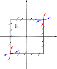
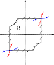
(a)	(b)

Figure 3. Regions $\Omega$ and $\mathcal{S}$.

Proof.

(i). Consider the function $f(x,y)=x-m^{-1/4}$. It is not difficult to see that $\langle\nabla f,X\rangle$ restricted to $x-m^{-1/4}=0$ has the expression $y^{3}-m^{-1/4}$ which is negative for $y\in(-m^{-1/4},m^{-1/4})$. Analogously, we can see that the direction of $X$ along $\partial\mathcal{S}$ is as showed in Figure 3 (a).

(ii). It is well-known that the sum of the indices of all the singularities surrounded by a periodic orbit, or a polycycle is one. Recall that the indices of the saddle points are $-1$ and the index of a monodromic point is $+1$. Hence, if a periodic orbit or a polycycle $\Gamma$ exist they must surround only the origin. Moreover, by statement (i), $\Gamma$ cannot intersect $\partial\mathcal{S}$. Finally, a simple computation shows that $\langle\nabla(xy+1),X\rangle$ restricted to $xy+1=0$ is $(1-m)/x^{4}$, which implies that $X$ is transversal to $xy+1=0$. Hence $X$ is transversal to $\partial\Omega$ and the lemma follows. ∎

Proposition 5.2.

For $m\in[1/2,3/5)$, system (1) has at most one limit cycle and one polycycle and both never coexist. Moreover, when the limit cycle exists it is hyperbolic and repeller.

Proof.

Following statement (ii) of Lemma 4.2 we take $k=2/3$ and a function $V_{2}(x,y)=g_{0}(y)+g_{1}(y)x+g_{2}(y)x^{2}$ adequate to apply Proposition 3.3 for proving the uniqueness of the limit cycles or polycycles for system (1).

We will take $g_{2}(y)$ as a truncated Taylor series at the origin of a suitable solution of (26) such that the curve $\{V_{2}=0\}$ has an oval surrounding the origin, and that $M_{2}$ does not change sign in $\Omega$. These two properties will imply the result.

The general solution of (26) is the linear combination of generalized hypergeometric functions

$$g_{2}(y)= \,C_{0}\sum_{j=0}^{\infty}\frac{\left(\phi^{+}(m)\right)_{j}\left(\phi^{-}(m)\right)_{j}}{\left(\frac{2}{3}\right)_{j}\left(\frac{5}{6}\right)_{j}}\left(\frac{m}{2}\right)^{j}\frac{y^{6j}}{j!}+C_{1}y\sum_{j=0}^{\infty}\frac{\left(\varphi^{+}(m)\right)_{j}\left(\varphi^{-}(m)\right)_{j}}{\left(\frac{5}{6}\right)_{j}\left(\frac{7}{6}\right)_{j}}\left(\frac{m}{2}\right)^{j}\frac{y^{6j}}{j!}$$

$$+C_{2}y^{2}\sum_{j=0}^{\infty}\frac{\left(\psi^{+}(m)\right)_{j}\left(\psi^{-}(m)\right)_{j}}{\left(\frac{7}{6}\right)_{j}\left(\frac{4}{3}\right)_{j}}\left(\frac{m}{2}\right)^{j}\frac{y^{6j}}{j!},$$ (27)

where $\phi^{\pm}(m)=\pm A(m)-2/9,$ $\varphi^{\pm}(m)=\pm A(m)-1/18,$ $\psi^{\pm}(m)=\pm A(m)+1/9,$ with $A(m)=\sqrt{(14m-3)/m}/9$.

We look for an even solution, so we take $C_{1}=0$. As we will consider $C_{0}\neq 0,$ it is not restrictive to choose $C_{0}=1$. Finally, the constant $C_{2}=-(3/5-m)^{2/3}$ is fixed after some previous simulations and taking into account that we already know that at $m=3/5$ there is a Hopf-like bifurcation.

Once we have fixed the above constants, we calculate the Taylor polynomial of degree 12 of $g_{2}$ at $y=0,$ $\mathcal{T}_{12}(g_{2})$, obtaining

$$\mathcal{T}_{12}(g_{2}(y))= \frac{1}{89100}(3-10m)(3+35m)y^{12}-\frac{1}{6300}(75-125m)^{2/3}(3-13m)y^{8}$$

$$+\frac{1}{90}(3-10m)y^{6}-\frac{1}{25}(75-125m)^{2/3}y^{2}+1.$$ (28)

So, in (ii) Lemma 4.2, we fix $g_{2}$ as $\mathcal{T}_{12}(g_{2}(y))$. Then the corresponding $g_{0}$ and $g_{1}$ are given by ((ii)). Thus, $M_{2}$ is of the form $M_{2}=(\phi(y)x+\psi(y))y^{4}$ where

$$\phi(y)= {\frac{1}{9450}}\Big{(}{\frac{7}{99}}\,\left(3-10\,m\right)\left(242\,m+3\right)\left(35\,m+3\right){y}^{11}$$

$$\qquad\quad+\left(75-125\,m\right)^{2/3}\left(86\,m+3\right)\left(13\,m-3\right){y}^{7}\Big{)},$$

$$\psi(y)= -{\frac{247}{400950}}\,{m}^{2}\left(3-10\,m\right)\left(35\,m+3\right){y}^{16}-{\frac{13}{4050}}\,{m}^{2}\left(75-125\,m\right)^{2/3}\left(13\,m-3\right){y}^{12}$$

$$+{\frac{1}{7425}}\,\left(3-10\,m\right)\left(550\,{m}^{2}+145\,m+3\right){y}^{10}$$

$$+{\frac{2}{4725}}\,\left(75-125\,m\right)^{2/3}\left(196\,{m}^{2}-45\,m-9\right){y}^{6}$$

$$+\frac{1}{15}\left(3-5\,m\right){y}^{4}-{\frac{2}{75}}\,\left(75-125\,m\right)^{2/3}\left(3-5\,m\right).$$

The proposition follows if we prove that $M_{2}$ does not change sign on the region $\Omega$. In fact, it is sufficient to prove that $M:=M_{2}/y^{4}$ does not change sign on $\Omega$.

The idea is to show that $\{M=0\}$ does not intersect $\Omega$. Since $M$ is linear in the variable $x$, $\{M=0\}$ cannot have ovals inside $\Omega$. If $\{M=0\}$ has a component in $\Omega$, this component would have to cross $\partial\Omega$ by continuity of the function. Then, it suffices to see that $\{M=0\}$ does not intersect $\partial\Omega$. Moreover, as $M$ satisfies $M(x,y)=M(-x,-y)$, it is sufficient to study $M$ on half of $\partial\Omega$. To deal only with polynomials we introduce the new variables $n=\sqrt[4]{m}$ and $s=(75-125m)^{2/3}$. Notice that $s^{3}=(75-125n^{4})^{2}.$

We split the half of the boundary of $\Omega$ in four pieces:

• The segment $\gamma_{1}=\{(x,1/n)\,:\,-n<x<1/n\},$

• The segment $\gamma_{2}=\{(1/n,y)\,:\,-n<y<1/n\},$

• The piece of hyperbola $\gamma_{3}=\{(x,-1/x)\,:\,n<x<1/n\},$

• The corners $\gamma_{4}=\{(1/n,1/n),(1/n,-n),(n,-1/n)\}$

and we have to prove that $\{M=0\}\cap\gamma_{i}=\emptyset$ for each $i=1,2,3,4.$

These facts can be seen proving that for $n\in I:=[\sqrt[4]{1/2},\sqrt[4]{3/5}\,)$,

• $Q_{1}(x,n,s):=M(x,1/n)\neq 0,$ for $x\in(-n,1/n)$.

• $Q_{2}(y,n,s):=M(1/n,y)\neq 0,$ for $y\in(-n,1/n)$.

• $Q_{3}(x,n,s):=M(x,-1/x)\neq 0,$ for $x\in(n,1/n)$.

• $M(1/n,1/n)\cdot M(1/n,-n)\cdot M(n,-1/n)\neq 0.$

Lemma 3.6, with $r=0$, is a convenient tool to prove the first three items. The proof of the last item is an straightforward consequence of Sturm method.

We will give the details of the proof that $Q_{2}(y,n,s)\neq 0$, which is the most elaborate case. The remainder two cases follow similarly.

Writing $Q(y,n,s):=2806650nQ_{2}(y,n,s)$ we get that

$$Q(y,n,s)= 1729\,n^{9}(35n^{4}+3)(10n^{4}-3)y^{16}-9009\,n^{9}s(13n^{4}-3)y^{12}$$

$$-21(10n^{4}-3)(242n^{4}+3)(35n^{4}+3)y^{11}$$

$$-378n(10n^{4}-3)(550n^{8}+145n^{4}+3)y^{10}+297s(13n^{4}-3)(86n^{4}+3)y^{7}$$

$$+1188ns(196n^{8}-45n^{4}-9)y^{6}-187110n(5n^{4}-3)y^{4}+74844ns(5n^{4}-3).$$

Looking at Lemma 3.6 with $r=0$, it suffices to prove the following three facts:

1. When $n=\sqrt[4]{1/2}\in I$, $Q(y,n,s)\neq 0$ for $y\in(-n,1/n)$.

2. For $n\in I$, $\triangle_{y}Q(y,n,s)\neq 0$.

3. For $n\in I$, $Q(-n,n,s)\cdot Q(1/n,n,s)\neq 0$.

Since the polynomial has no rational coefficients the proof of item (i) requires some special tricks. Notice that when $n=\sqrt[4]{1/2}$ then $s=5\sqrt[3]{10}/2$. Hence,

$$R(y):=Q\Big{(}y,\frac{1}{\sqrt[4]{2}},\frac{5}{2}\sqrt[3]{10}\Big{)}= {\frac{70889}{8}}\sqrt[4]{8}\,{y}^{16}-{\frac{315315}{32}}\sqrt[4]{8}\sqrt[3]{10}\,{y}^{12}-106764{y}^{11}$$

$$-80514\,\sqrt[4]{8}\,{y}^{10}+{\frac{239085}{2}}\sqrt[3]{10}\,{y}^{7}+{\frac{51975}{2}}\sqrt[4]{8}\sqrt[3]{10}\,{y}^{6}$$

$$+{\frac{93555}{2}}\sqrt[4]{8}\,{y}^{4}-{\frac{93555}{2}}\sqrt[4]{8}\sqrt[3]{10}.$$

We will prove that the above polynomial has no real roots in $[-1,12/10]\supset(-n,1/n).$ The Sturm method gives polynomials with huge coefficients and our computers have problems to deal with them. We use a different approach. We know, that

$$\underline{n}:=\dfrac{3002}{1785}<\sqrt[4]{8}<\dfrac{37}{22}=:\overline{n},\quad\underline{s}:=\dfrac{28}{13}<\sqrt[3]{10}<\dfrac{265}{123}=:\overline{s},$$

where these four rational approximations are obtained computing the continuous fraction expansion of both irrational numbers. If we construct the polynomial, with rational coefficients,

$$R^{+}(y)= {\frac{70889}{8}}\overline{n}\,{y}^{16}-{\frac{315315}{32}}\underline{n}\,\underline{s}\,{y}^{12}-106764{y}^{11}-80514\underline{n}\,{y}^{10}$$

$$+{\frac{239085}{2}}\overline{s}\,{y}^{7}+{\frac{51975}{2}}\overline{n}\,\overline{s}\,{y}^{6}+{\frac{93555}{2}}\overline{n}\,{y}^{4}-{\frac{93555}{2}}\underline{n}\,\underline{s},$$

it is clear that for $y\geq 0,$ $R(y)<R^{+}(y).$ In fact,

$$R^{+}(y)= {\frac{2622893}{176}}{y}^{16}-{\frac{2427117}{68}}{y}^{12}-106764{y}^{11}-{\frac{11509668}{85}}{y}^{10}$$

$$+{\frac{21119175}{82}}{y}^{7}+{\frac{15442875}{164}}{y}^{6}+{\frac{314685}{4}}{y}^{4}-{\frac{37446948}{221}}$$

and, now, using the Sturm method it is quite easy to prove that $R^{+}(y)<0$ for $y\in[0,12/10].$ Hence, in this interval, $R(y)<R^{+}(y)<0,$ as we wanted to prove.

To study the values of $y<0$ we construct a similar upper bound,

$$R^{-}(y)= {\frac{70889}{8}}\overline{n}\,{y}^{16}-{\frac{315315}{32}}\underline{n}\,\underline{s}\,{y}^{12}-106764{y}^{11}-80514\underline{n}\,{y}^{10}$$

$$+{\frac{239085}{2}}\underline{s}\,{y}^{7}+{\frac{51975}{2}}\overline{n}\,\overline{s}\,{y}^{6}+{\frac{93555}{2}}\overline{n}\,{y}^{4}-{\frac{93555}{2}}\underline{n}\,\underline{s},$$

and applying the same method the result follows.

To prove (ii) we compute

$$\triangle_{y}Q(y,n,s)=n^{42}s^{3}(5n^{4}-3)^{5}(35n^{4}+3)^{3}(10n^{4}-3)^{3}P_{258}(n,s),$$

where $P_{258}(n,s)$ is a polynomial in $n$ and $s$ of degree 258. Clearly, the roots of the first five factors of the above discriminant are no relevant for our problem because the corresponding $n$ is not in $I.$ To study whether $P_{258}(n,s)$ vanishes or not we compute

$$\operatorname{Res}(P_{258}(n,s),(75-125n^{4})^{2}-s^{3},s)=(5n^{4}-3)^{24}{P}_{390}(n^{2}),$$

where ${P}_{390}(n^{2})$ is a polynomial of degree 390 in $n^{2}$. Applying again the Sturm method we get that ${P}_{390}(n^{2})$ has no significant roots for our study. Finally, the numerator of $Q(-n,n,s)\cdot Q(1/n,n,s)$ is a polynomial in $n$ and $s$ of degree 49. Using the same trick as above we prove item (iii). In this case the polynomial we have to deal with has degree 152 in $n$.

Therefore $\{M=0\}\cap\partial\Omega=\emptyset$ and as a consequence $\{M=0\}\cap\Omega=\emptyset$.

Finally, it is not difficult to see, because $V$ is quadratic in $x,$ that the set $\{V(x,y)=0\}$ has exactly one oval surrounding the origin. Hence, the proposition follows. ∎

Proof of Proposition 1.2.

Notice that the function $V$ used in the proof of Proposition 5.2 coincides with the function $V(x,y,m)$ of the statement of the proposition. Taking $k=2/3$ we are also under the hypotheses of Corollary 3.4. Therefore the set $\mathcal{U}_{m}$ is contained in $\mathcal{W}^{s}_{\bf 0}$, as we wanted to prove. ∎

We remak that following similar ideas that in the above proof we can construct bigger sets contained in $\mathcal{W}^{s}_{\bf 0}$. For a given $m$, let us denote by $\mathcal{T}_{\ell}(g_{2}(x;C_{2}))$ the Taylor polynomial of degree $\ell$ at $x=0$, of the function (5) with $C_{0}=1,$ $C_{1}=0.$ Then for each $\ell\in\mathbb{N}$ and $C_{2}\in\mathbb{R}$ we can take this function as a new seed $g_{2}$ for constructing the corresponding $V$ as in (ii) of Lemma 4.2. Then checking that the oval contained in $\{V=0\}$ is crossed inwards by the flow of the system, the result follows for the function $V$ constructed with these $\ell$ and $C_{2}$.

6. Non-existence of limit cycles and polycycles for $m\in(9/25,0.547]$

This section contains new non-existence results for system (1). We split the interval into the subintervals $(9/25,1/2)$ and $[1/2,0.547]$. Recall that our numerical study shows that the system has no limit cycles for $m<0.56011\ldots$ As $m$ becomes closer to this bifurcation value the proof of non-existence of periodic orbits and polycycles becomes harder.

Proposition 6.1.

For $m\in(9/25,1/2)$, system (1) has neither limit cycles nor polycycles.

Proof.

We would like to apply Proposition 3.3. To this end we will follow similar steps that in the proof of Proposition 5.2, but with a function $V$ such that the set $\{V=0\}$ has no oval in $\Omega.$ Recall that $\Omega$ is the domain introduced in Lemma 5.1, where the limit cycles and the polycycles must lay. We take $V=V_{2}(x,y)=g_{0}(y)+g_{1}(y)x+g_{2}(y)x^{2}$ with $g_{1}(y)=g_{2}^{\prime}(y)$, $g_{0}=(1/2)g_{2}^{\prime\prime}(y)-(1/2)my^{5}g_{2}^{\prime}(y)+(5/3)my^{4}g_{2}(y)$. Now we consider $g_{2}(y)=a_{0}+a_{2}y^{2}+a_{4}y^{4}+a_{6}y^{6}+a_{8}y^{8}$, with coefficients to be determined. From statement (ii) of Lemma 4.2 it follows that the corresponding $M_{2}$ is a polynomial function in $x$ of the form $M_{2}=\phi(y)x+\psi(y)$ where $\phi(y)$ and $\psi(y)$ are polynomials in the variable $y$ whose coefficients depend on $a_{2j}$, $j=0,1,\ldots,4$. In order to simplify the computations, we change the parameter $m$ by $n^{4}$ to transform $V$ into a polynomial in the variables $x$, $y$, and $n$. Since $m\in(9/25,1/2)$ we can restrict our study to $n\in(0.77,0.844)$.

We consider the values of $a_{4},a_{6}$ and $a_{8}$ such that $\phi(y)$ has a zero at $y=0$ of multiplicity nine, we choose the value of $a_{2}$ by imposing that $M_{2}$ vanishes at the two saddle points of the system and, finally, we use the freedom of changing $g_{2}(y)$ by $\lambda g_{2}(y),$ for any $0\neq\lambda\in\mathbb{R}$, to remove all the denominators. We obtain that

$${g}_{2}(y)= 270(9+51n^{2}+213n^{4}+535n^{6}+924n^{8}+756n^{10})$$

$$-756n^{2}(9+42n^{2}+105n^{4}+130n^{6})y^{2}$$

$$+3(3-10n^{4})(9+51n^{2}+213n^{4}+535n^{6}+924n^{8}+756n^{10})y^{6}$$

$$-3n^{2}(3-13n^{4})(9+42n^{2}+105n^{4}+130n^{6})y^{8}.$$

The corresponding $M_{2}$ is of the form

$$M_{2}(x,y)=\frac{2}{3}y^{4}\,(\phi(y)x+\psi(y))=:\frac{2}{3}y^{4}\,M(x,y),$$ (29)

where

$$\phi(y)= 3(3-10n^{4})(3+35n^{4})(9+51n^{2}+213n^{4}+535n^{6}+924n^{8}+756n^{10})y^{5}$$

$$-3n^{2}(3-13n^{4})(3+86n^{4})(9+42n^{2}+105n^{4}+130n^{6})y^{7},$$

$$\psi(y)= -756n^{2}(3-5n^{4})(9+42n^{2}+105n^{4}+130n^{6})$$

$$+27(3-5n^{4})(9+51n^{2}+213n^{4}+535n^{6}+924n^{8}+756n^{10})y^{4}$$

$$-12n^{2}(9+42n^{2}+105n^{4}+130n^{6})(9+45n^{4}-196n^{8})y^{6}$$

$$-40n^{8}(3-10n^{4})(9+51n^{2}+213n^{4}+535n^{6}+924n^{8}+756n^{10})y^{10}$$

$$+91n^{10}(3-13n^{4})(9+42n^{2}+105n^{4}+130n^{6})y^{12}.$$

Recall that the main hypothesis in Proposition 3.3 is that $M$ does not change on $\Omega$. As we will see, this happens only for $n\in J:=(0.77,\widetilde{n}]$ where $\widetilde{n}\approx 0.8045592$ will be precisely defined afterwards. When $n\in K:=(\widetilde{n},0.844)$ the result will be a consequence of the variation of Proposition 3.3 described in Remark 3.5.

For $n\in J$, following similar steps that in the proof of Proposition 5.2, we divide half of the boundary of $\Omega$ in five pieces:

• The segment $\gamma_{1}=\{(x,1/n)\,:\,-n<x<1/n\},$

• The segment $\gamma_{2}=\{(1/n,y)\,:\,-n<y<1/n\},$

• The piece of hyperbola $\gamma_{3}=\{(x,-1/x)\,:\,n<x<1/n\},$

• The corners $\gamma_{4}=\{(1/n,-n),(n,-1/n)\}$,

• The corner $\gamma_{5}=\{(1/n,1/n)\}$

and we will prove that $\{M=0\}\cap\gamma_{i}=\emptyset$ for each $i=1,2,3,4$ and that although $(1/n,1/n)\in\partial\Omega$, the set $\{M=0\}$ does not enter in $\Omega.$ From these results we will have proved that $M$ does not change sign on $\Omega$ and, as a consequence, the proposition will follow for $n\in J.$

To prove the fifth assertion it suffices to study the function $M$ in a neighborhood of the point $(1/n,1/n)\in\partial\Omega$. By the construction of $M$, it holds that $M(1/n,1/n)=0$. By computing the partial derivatives of $M$ at this point we obtain which is the tangent vector of the curve at $(1/n,1/n)$. Then, it is easy to see that when $n\in J$, in a punctured neighborhood $\mathcal{W}$ of $(1/n,1/n)$, it holds that $\mathcal{W}\cap\{M=0\}\cap\,\Omega=\emptyset$. In fact, $\widetilde{n}\in\partial J$ is a solution of the equation

$$\operatorname{num}\Big{(}\frac{\partial M(x,y)}{\partial x}\Big{|}_{(x,y)=(1/n,1/n)}\Big{)}=0,$$

where $\operatorname{num}(\cdot)$ denotes the numerator of the rational function. Moreover,

$$M\Big{(}x,\frac{1}{n}\Big{)}=-\frac{9(nx-1)}{n^{4}} \Big{(}88200{n}^{16}+107800{n}^{14}-4930{n}^{12}$$

$$-37380{n}^{10}-15855{n}^{8}-2736{n}^{6}+576{n}^{4}+108{n}^{2}-27\Big{)}$$ (30)

and $\widetilde{n}$ is also the positive root of the polynomial in $n$ appearing in the right-hand side of the above formula. Notice that when $n=\widetilde{n}$, the straight line $\{y=1/\widetilde{n}\}$ is a subset of $\{M=0\}.$ This fact is the reason for which this approach only works for $n\in J=(0.77,\widetilde{n}]$.

Let us prove the remainder four assertions. As in the proof of Proposition 5.2, they follow by showing that when $n\in J$,

• $R_{1}(x,n):=\operatorname{num}(M(x,1/n))\neq 0,$ for $x\in(-n,1/n)$.

• $R_{2}(y,n):=\operatorname{num}(M(1/n,y))\neq 0,$ for $y\in(-n,1/n)$,

• $R_{3}(x,n):=\operatorname{num}(M(x,-1/x))\neq 0,$ for $x\in(n,1/n)$.

• $M(1/n,-n)\cdot M(n,-1/n)\neq 0.$

That $R_{1}$ has no zeros in $J$, is an straightforward consequence of (6).

To study $R_{2}$ and $R_{3}$ we will use Lemma 5.1. We start computing the discriminants,

$$S_{2}(n)=\triangle_{y}(R_{2}(y,n)),\quad S_{3}(n)=\triangle_{x}(R_{3}(x,n)),$$

and analyze whether they vanish or not on $J.$ Using the Sturm method we get that on $J$, $S_{2}$ vanishes only at one value $n_{2}\approx 0.8040188$ and $S_{3}$ also vanishes only at one value $n_{3}\approx 0.8045576.$ The root $n_{2}$ of $S_{2}$ forces to split the study of $R_{2}(y,n)$ in the three subcases: $n\in(0.77,n_{2})$, $n=n_{2}$ and $n\in(n_{2},\widetilde{n}]$. Doing the same type of computations and reasoning as in the previous section we can prove all the above assertion when $n\neq n_{2}$. The case $n=n_{2}$ follows by continuity arguments, because it can be seen that in this situation $R_{2}$ has a real multiple root but it is not in $(-n_{2},1/n_{2})$. The study of $R_{3}$ is similar to the one of $R_{2}$ and we omit it. We also get that $R_{3}$ neither vanishes on $(n,1/n).$

That for $n\neq\widetilde{n}$, $M(1/n,-n)\cdot M(n,-1/n)\neq 0$ is once more a consequence of the Sturm method.

Therefore, when $n\in J,$ we are under the hypotheses of Proposition 3.3, and we will know that the system has no limit cycles once we have proved that the set $\{V=0\}$ has no ovals. We defer the proof of this fact until we have considered the case $n\in K=(\widetilde{n},0.844)$.

When $n\in K,$ we know that $\{M=0\}\cap\,\Omega\neq\emptyset$ and we are no more under the hypotheses of Proposition 3.3. Let us see that we can apply the ideas of Remark 3.5. To this end we have to prove that $\{M_{2}=0\}^{*}\cap\Omega$ is without contact for the flow of $X$. Note that $\{M_{2}=0\}^{*}=\{M=0\}^{*}$.

We need to show that $\dot{M}=\langle\nabla M,X\rangle$ does not vanish on $\{M=0\}^{*}\cap\Omega$. We study the common points of $\{M=0\}$ and $\{\dot{M}=0\}$ and prove that they are not in $\Omega.$ First, we compute

$$\dot{M}(x,y)=\langle\nabla M(x,y),X(x,y)\rangle=:y^{3}N(x,y),$$

and we remove the factor $y^{3}.$ We do not care about the points on $\{y=0\}$ because

$$M(x,0)=756{n}^{2}\left(5{n}^{4}-3\right)\left({9}+42{n}^{2}+105{n}^{4}+130{n}^{6}\right)\neq 0,$$

for $n\in(0,0.88].$

The resultant $\operatorname{Res}(M,N,x)$ factorizes as

$$\operatorname{Res}(M,N,x)=y^{2}(n^{2}y^{2}-1)(P_{n,2}(y))(P_{n,34}(y)),$$

where $P_{n,2}(y)$ and $P_{n,34}(y)$ are polynomials in the variable $y$ with respective degrees 2 and 34 and whose coefficients are polynomial functions with rational coefficients in the variable $n$.

Clearly, $(n^{2}y^{2}-1)$ does not vanish on $-1/n<y<1/n$. By using once more Lemma 3.6 it is not difficult to prove that $P_{n,2}(y)$ does not vanish either on $-1/n<y<1/n$, for $n\in(\widetilde{n},0.844)$. Hence we will focus on the factor $P_{n,34}(y)$.

We will use again Lemma 3.6. By using the Sturm method we get that $\triangle_{y}(P_{n,34}(y))$ has no zeros in the interval $K$. In fact one zero is $\widetilde{n}\in\partial K$ and another one is $n^{*}\approx 0.8445\not\in J$ and this is the reason for which we can only prove the result until $n=0.844<n^{*}.$ By using Sturm method, it can be shown that $P_{n,34}(-1/n)\cdot P_{n,34}(1/n)\not=0$ for all $n\in K$ and, for instance, for $n=n_{0}=83/100\in K$, the polynomial $P_{n_{0},34}(y)$ has exactly two (simple) zeros in $-1/n_{0}<y<1/n_{0}$. Then, Lemma 3.6 with $r=2,$ implies that $P_{n,34}(y)$ has exactly two (simple) zeros in $-1/n<y<1/n$, for all $n\in K$. We call them $y=y_{i}(n),i=1,2$ and they are continuous function of $n$. Therefore, we need to prove that the corresponding points in $\{M=0\}\cap\{N=0\}$ are outside of $\Omega$.

Notice that because of the expression of $M$, given in (29), the points in $\{M=0\}$ are on the curve $\Gamma=\{\big{(}-\frac{\psi(y)}{\phi(y)},y\big{)}\,:\,y\in\mathbb{R}\setminus\{0\}\}$. Moreover it can be easily seen that $\phi(y)\neq 0$ on the region that we are considering. Therefore the points in $\{M=0\}\cap\{N=0\}$ are given by the two continuous curves

$$\gamma_{i}:=\Big{\{}\Big{(}-\dfrac{\psi(y_{i}(n))}{\phi(y_{i}(n))},y_{i}(n)\Big{)}\,:\,n\in K\Big{\}},\quad i=1,2.$$

For a fixed $n\in K$ it is not difficult to prove that the points in $\gamma_{i},i=1,2$ are outside of $\Omega$. If for some $n\in K$ there was a point inside $\Omega$, by continuity it would be at least one point in one of the pieces of boundary of $\Omega$ formed by the straight line $\{x-1/n=0\}$ and the hyperbola $\{xy+1=0\}$. To prove that such a point does not exist we compute the following two resultants

$$\operatorname{Res}\Big{(}\operatorname{num}\Big{(}-\dfrac{\psi(y)}{\phi(y)}-\dfrac{1}{n}\Big{)},P_{n,34}(y),y\Big{)}=P_{1250}(n),$$

$$\operatorname{Res}\Big{(}\operatorname{num}\Big{(}-y\dfrac{\psi(y)}{\phi(y)}+1\Big{)},P_{n,34}(y),y\Big{)}=P_{1260}(n),$$

where $P_{\ell}(n)$ are given polynomials with rational coefficients and degree $\ell$. Both polynomials factorize in several factors and, using once more the Sturm method, we can easily prove that do not vanish on $K$. Hence, $\{M=0\}\cap\{N=0\}\cap\Omega=\emptyset$ which implies that $\{M=0\}\cap\Omega$ is without contact by the flow of $X$, as we wanted to prove.

Since $M$ is linear in the variable $x$, $\{M=0\}$ cannot have ovals. Therefore, by Remark 3.5, to end the proof we need to show that the set $\{V=0\}$ has no ovals either in $\Omega.$ We claim that the set $\{V=0\}\cap\,\Omega$ is without contact by the flow of the system. If this happens and $\{V=0\}$ had an oval then it would be without contact. Then by the Poincaré-Bendixson Theorem it should surround the origin. However, by considering the straight line passing through the origin $y=9x/10$ it is easy to prove, by using again Lemma 3.6, that the function $V(x,9x/10)$ does not vanish on the interval $-1/n<x<1/n$ for all $n\in(0.77,0.844)$. Thus, $\{V=0\}\cap\{y-9x/10=0\}=\emptyset$. Hence, $V$ has no ovals inside $\Omega$ as we wanted to see and the proposition follows by using all the above results and the reasoning explained in Remark 3.5.

To prove the above claim, it suffices to see that $\{M=0\}\cap\{V=0\}\cap\Omega=\emptyset$. This is because precisely, $M\big{|}_{\{V=0\}}=\dot{V}.$

Recall that when $n\in J=(0.77,\widetilde{n}]$ then $\{M=0\}\cap\Omega=\emptyset$ and so the result follows.

Let us consider the case $n\in K=(\widetilde{n},0.844)$. To study if $\{V=0\}$ and $\{M=0\}$ intersect, we compute the resultant of $M$ and $V$ with respect to $x$. We have

$$\operatorname{Res}(V,M,x)=(n^{2}y^{2}-1)P_{n,30}(y),$$

where $P_{n,30}(y)$ is a polynomial of degree 30 and whose coefficients are polynomial functions in the variable $n$ with rational coefficients. We want to prove that $\operatorname{Res}(V,M,x)$ does not vanish on the interval $-1/n<y<1/n$ for $n\in K$. It suffices to study $P_{n,30}(y)$. We will use once more Lemma 3.6.

The polynomial $P_{n,30}(-1/n)\cdot P_{n,30}(1/n)$ has no real roots when $n\in K$. Moreover hypothesis (i) of Lemma 3.6 holds with $r=0$ (no real roots) by considering for instance $n_{0}=82/100$. To see that condition (iii) of the lemma holds, we compute $\triangle_{y}(P_{n,30}(y))$. It is a polynomial of degree $2728$ in the variable $n$ which factorizes in several factors, being the largest one of degree 594. From this decomposition we can prove that $\triangle_{y}(P_{n,30}(y))$ has no zeros for $n\in K$. Therefore, by Lemma 3.6 we conclude that $P_{n,30}(y)$ does not vanish on the whole interval $-1/n<y<1/n$ for $n\in K$, and the claim follows. ∎

Proposition 6.2.

For $m\in[0.5,0.547]$, system (1) has neither limit cycles nor polycycles.

Proof.

We will construct a positive invariant region $\mathcal{R}$ having the two saddle points in its boundary. As we will see, the proposition follows once we have constructed this region, simply by using the uniqueness and hyperbolicity of the limit cycle, whenever it exits. We remark that in this proof we will not use the Bendixson-Dulac theorem.

Assume that such a positive invariant region $\mathcal{R}$ exits. By the Index theory, if the system had a limit cycle, it should surround only the origin. By Proposition 5.2 we already know that for $n\in[0.5,0.6)\supset L:=[0.5,0.547]$, the limit cycle would be unique, hyperbolic and repeller. By the Bendixson-Poincaré Theorem the above facts force the existence of another limit cycle and so a contradiction. It is straightforward that the existence of this positive invariant region is not compatible with the existence of a polycycle connecting both saddle points.

To construct $\mathcal{R}$ we consider a function $V_{2}(x,y)=g_{0}(y)+g_{1}(y)x+g_{2}(y)x^{2}$, with $g_{0}$ and $g_{1}$ as in ((ii)) and $g_{2}$ an even polynomial function of degree 12 of the form

$$g_{2}(y)=1+\sum_{k=1}^{6}a_{2k}y^{2k},$$

to be determined. By statement (ii) of Lemma 4.2, the function $M_{2}$, given in ((ii)), associated to this $V_{2}$ and $k=2/3$ is of the form $M_{2}=\phi(y)x+\psi(y)$, where $\phi(y)$ and $\psi(y)$ are polynomials in the variable $y$ whose coefficients depend on the unknowns $a_{2k}$ with $k=1\ldots 6$.

We fix $a_{4}$ and $a_{6}$ in such a way that $\phi(y)$ has a zero at $y=0$ of multiplicity nine; we get the value of $a_{8}$ by imposing that $V_{2}$ vanishes at the two saddle points; the values of $a_{2}$ and $a_{10}$ are chosen so that the curve $V_{2}=0$ is tangent to both separatrices at the saddle points of the system. Finally, after experimenting with several values for $a_{12}$ and $m$, so that the region with boundary $\{V_{2}=0\}$ is positively invariant, we fix $a_{12}=-157(10m-3)(35m+3)/44550000$.

The region $\mathcal{R}$ will be the bounded connected component of $\mathbb{R}^{2}\setminus\{V_{2}=0\}$ containing the origin, see Figure 4 $(a)$.

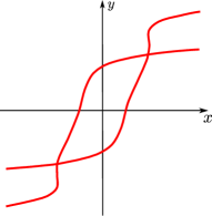
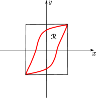
(a)	(b)

Figure 4. Positively invariant region $\mathcal{R}$ with boundary $\{V_{2}=0\}$.

We need to prove that the curve $\{V_{2}=0\}\cap\mathcal{S}$ (see Figure 4 (b)) is such that the vector field $X$ points in on all its points. We introduce the new parameter $m=n^{2}$ and we compute $\dot{V_{2}}=\langle\nabla V_{2},X\rangle$ and

$$\operatorname{Res}(V_{2},\dot{V_{2}},x)=\frac{y^{8}(ny^{2}-1)^{4}(P_{n,12}(y))^{3}P_{n,36}(y)}{n^{28}(120n^{3}+113n^{2}-3)^{6}},$$ (31)

where $P_{n,12}(y)$ and $P_{n,36}(y)$ are polynomials of degree 12 and 36, respectively, and whose coefficients are polynomial functions in the variable $n$.

Notice that since $m\in[0.5,0.547]$ then $n\in T:=[0.707,0.7396]$. Since the denominator of (31) is positive, we only need to study its numerator.

Using once more Lemma 3.6 and the same tools that in the previous sections we prove that $P_{n,12}(y)\cdot P_{n,36}(y)$ is positive for all $y\in(-1/n,1/n)$ and $n\in T.$ We omit the details.

Hence, we have proved that the numerator of $\operatorname{Res}(V_{2},\dot{V_{2}},x)$ is non-negative and it only vanishes on $y=0$ and $y=\pm n^{-1/2}$. Therefore the sets $\{V_{2}=0\}$ and $\{\dot{V}_{2}=0\}$ only can intersect on $\{y=0\}.$ Indeed, the sets $\{V_{2}=0\}\cap\mathcal{S}\cap\{y=0\}$ and $\{\dot{V}_{2}=0\}\cap\mathcal{S}\cap\{y=0\}$ coincide and have two points $(\pm\widehat{x}(n),0)$ for each $n\in T.$ Studying the local Taylor expansions of $V_{2}(x,y)$ and $\dot{V}_{2}(x,y)$ at these points we get that the respective curves $V_{2}(x,y)=0$ and $\dot{V}_{2}(x,y)=0$ have at them a fourth order contact point and, as a consequence, $\dot{V}_{2}$ does not change sign on $\{V_{2}=0\}\cap\mathcal{S}$, as we wanted to prove. That, on $\{V_{2}=0\}$, the vector field $X$ points in, is a simple verification. Hence the proof follows.∎

7. Existence of polycyles

This section is devoted to prove that the phase portrait (b) in Figure 1 can only appear for finitely many values of $m$. Notice that this phase portrait is precisely the only one presenting a polycycle. As we have already explained, the main difficulty is that we are dealing with a family that is not a SCFRVF. To see that the control of the existence of polycycles for general polynomial 1-parameter families can be a non easy task, we present a simple family for which a polycycle appears at least for two values of the parameter.

Example 7.1.

For $m=0$ and $m=1$, the planar systems

$$\left\{\begin{array}[]{lll}\dot{x}=-2y+(3m-4)x+(4-2m)x^{3}+xy^{2}-x^{5}=P_{m}(x,y),\\ \dot{y}=(4-m)x+xy^{2}-2mx^{3}-x^{5}=Q_{m}(x,y),\qquad m\in\mathbb{R}.\end{array}\right.$$ (32)

have a heteroclinic polycycle connecting the saddle points located at $(\pm\sqrt{2-m},0)$.

Proof.

The above family has been cooked to have explicit algebraic polycycles. Consider the family of algebraic curves $H_{m}(x,y)=y^{2}-(x^{2}+m-2)^{2}=0$ and compute

$$W_{m}(x,y)=\langle\nabla H_{m}(x,y),(P_{m}(x,y),Q_{m}(x,y))\rangle.$$

Doing the resultant with respect to $x$ of $W_{m}$ and $H_{m}$ we obtain

$$\operatorname{Res}(W_{m}(x,y),H_{m}(x,y),x)=m^{4}(1-m)^{4}y^{4}R(y,m),$$

where $R$ is a polynomial of degree 4 in both variables, $m$ and $y$. This implies that for $m=0$ and $m=1$ the algebraic curve $H_{m}(x,y)=0$ is invariant by the flow of (32). These sets coincide with the invariant manifolds of the saddle points $(\pm\sqrt{2-m},0)$ and contain the corresponding heteroclinic polycycles. ∎

We have simulated the phase portraits of (32) for several values of $m$ and it seems that no polycycles appear for other values of $m$. In any case, the example shows the differences between SCFRVF, for which as we have discussed in Subsection 3.1, the polycycle usually appears for a single value of the parameter, and families that are not SCFRVF.

Let us continue our study of system (1). We denote by ${\bf p}_{m}^{\pm}=(\pm m^{-1/4},\pm m^{-1/4})$ the two saddle points of the system.

Proposition 7.2.

Let $(0,y^{s}(m))$ be the first cut of the stable manifold of ${\bf p}_{m}^{+}$ with the $Oy^{+}$-axis. Similarly, let $(0,y^{u}(m))$ be the first cut of the unstable manifold of ${\bf p}_{m}^{-}$ with the same axis, see Figure 5 (a). Then the function $\delta(m):=y^{s}(m)-y^{u}(m)$ is an analytic function.

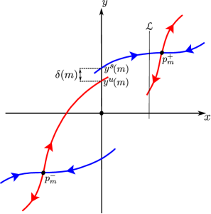
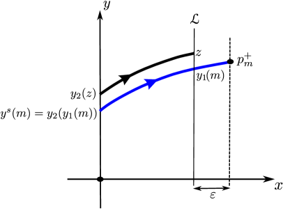
(a)	(b)

Figure 5. Definition of the maps $\delta(m)$ and $y^{s}(m)$ in Proposition 7.2.

Proof.

This result is a consequence of the tools introduced in [21]. We only give the key points of that proof.

Fix a value $\widehat{m}$ for which $\delta(m)$ is defined. Simply because the $Oy^{+}$ is transversal for the flow, the function $\delta$ is well defined in a neighborhood of $\widehat{m}.$ It is clear that it suffices to prove that $y^{s}(m)$ is analytic at $m=\widehat{m},$ because the $y^{u}(m)$ can be studied similarly. To prove this fact we will write the map $y^{s}(m)$ as the composition of two analytic maps.

Consider a vertical straight line $\mathcal{L}:=\{(x,y)\,:\,x=\widehat{m}^{-1/4}-\varepsilon\}$, for $\varepsilon>0$ small enough. Denote by $(\widehat{m}^{-1/4}-\varepsilon,y_{1}(m))$ the first cutting point of the stable manifold of ${\bf p}_{m}^{+}$ with this line. Because $\mathcal{L}$ is close enough to the saddle point it can be seen that the local stable manifold cuts this line transversally. Moreover, the tools given in [21] prove that $y_{1}(m)$ is analytic at $m=\widehat{m},$ because of the hyperbolicity of the saddle point. Next, consider the orbit starting on $\mathcal{L}$ with $y$-coordinate $y_{1}(\widehat{m})$. In backward time, this orbit cuts also transversally the $Oy^{+}$-axis at the point with $y$-coordinate $y^{s}(\widehat{m})$ and needs a finite time to arrive to this point see Figure 5 (b). Because of the transversality to both lines, and the finiteness of the needed time for going from one to the other, it is clear that the map $y_{2}(z)$ induced by the flow of the system between $\mathcal{L}$ and the $Oy^{+}$-axis is analytic at $z=y_{1}(\widehat{m})$. Since $y^{s}(m)=y_{2}(y_{1}(m))$, the result follows. ∎

Proof of (iii) of Theorem 1.1.

Notice that each value of $m$ that is a zero of the map $\delta(m),$ introduced in Proposition 7.2, corresponds to a system (1) with a polycycle, i.e. $\mathcal{M}=\{m\in(0.547,0.6)\,:\,\delta(m)=0\}.$ From Proposition 6.2 we know that $\delta(0.547)>0$ and from Proposition 4.4 that $\delta(0.6)<0.$ Hence the set $\mathcal{M}$ is non-empty. Finally, because of the non-accumulation property of the zeros of analytic functions, the finiteness of $\mathcal{M}$ follows. ∎

8. Proof of Theorem 1.1

The proof of Theorem 1.1 simply consists in gluing the corresponding results proved along the paper. More concretely:

• The non existence of limit cycles and polycycles when $m\in(-\infty,0.547]\cup[3/5,\infty)$ is given in the following results:

  • For $m\in(-\infty,0]$, trivially in the introduction.

  • For $m\in(0,9/25]$ in Proposition 4.1,

  • For $m\in(9/25,1/2)$ in Proposition 6.1,

  • For $m\in[1/2,0.547]$ in Proposition 6.2,

  • For $m\in[3/5,\infty)$ in Proposition 4.4.

• The existence of at most one limit cycle and one polycycle when $m\in[1/2,3/5)$, the fact that they never coexist, and the hyperbolicity and instability of the limit cycle, in Proposition 5.2.

• The phase portraits of the system in the Poincaré disc and the study of the origin, in Subsection 3.2 and Section 2, respectively.

• The proof of the existence of the phase portrait (b) in Figure 1, only for finitely many values of $m$, in Section 7.

Acknowledgements

The first two authors are supported by the MICIIN/FEDER grant number MTM2008-03437 and the Generalitat de Catalunya grant number 2009-SGR 410. The first author is also supported by the grant AP2009-1189.

References

- [1] M. Abramowitz, I. A. Stegun, “Handbook of Mathematical Functions with Formulas, Graphs, and Mathematical Tables” New York: Dover, eds. (1965).
- [2] M. J. Álvarez, A. Gasull, Monodromy and stability for nilpotent critical points. Internat. J. Bifur. Chaos Appl. Sci. Engrg. 15 (2005), 1253–1265.
- [3] A. A. Andronov, E. A. Leontovich, I. I Gordon. and A. G. Maier , “Qualitative theory of second-order dynamic systems”, John Wiley & Sons, New York (1973).
- [4] S. B. S. D., Castro, The disappearance of the limit cycle in a mode interaction problem with symmetry. Nonlinearity 10 (1997), 425–432.
- [5] L. A. Cherkas, The Dulac function for polynomial autonomous systems on a plane, (Russian) Differ. Uravn. 33 (1997), 689–699, 719; translation in Differential Equations 33 (1997), 692–701.
- [6] B. Coll, A. Gasull, R. Prohens, Differential equations defined by the sum of two quasi-homogeneous vector fields. Canad. J. Math. 49 (1997), 212–231.
- [7] D. Cox, J. Little, D. O’Shea, “Using algebraic geometry”, New York [etc.]: Springer–Verlag, (1998).
- [8] G. Dangelmayr, J. Guckenheimer, On a four parameter family of planar vector fields. Arch. Rational Mech. Anal. 97 (1987), 321 -352.
- [9] G. F. D. Duff, Limit-cycles and rotated vector fields. Ann. of Math. 57, (1953), 15–31.
- [10] M. Galeotti, F. Gori, Bifurcations and limit cycles in a family of planar polynomial dynamical systems, Rend. Sem. Mat. Univ. Politec. Torino, (1), 46 (1988), 31–58.
- [11] J. D. García-Saldaña, A. Gasull, H. Giacomini, Bifurcation values for a family of planar vector fields of degree five, Preprint 2012.
- [12] A. Gasull, H. Giacomini, Upper bounds for the number of limit cycles of some planar polynomial differential systems, Discrete Contin. Dyn. Syst., 27 (2010) 217–229.
- [13] A. Gasull, H. Giacomini, A new criterion for controlling the number of limit cycles of some generalized Liénard equations, J. Differential Equations, 185 (2002) 54–73.
- [14] A. Gasull, H. Giacomini, J. Torregrosa, Some results on homoclinic and heteroclinic connections in planar systems, Nonlinearity 23, (2010), 2977–3001.
- [15] A. Gasull, J. Torregrosa, A new algorithm for the computation of the Lyapunov constants for some degenerate critical points, Nonlin. Anal. 47, (2001) 4479–4490.
- [16] N. G. Lloyd, A note on the number of limit cycles in certain two-dimensional systems, J. London Math. Soc.(2), 20 (1979) 277–286.
- [17] A. M. Lyapunov, “Stability of motion”, Mathematics in Science and Engineering, 30, Academic Press, New York, London (1966).
- [18] L. Markus, Global structure of ordinary differential equations in the plane, Trans. Amer. Math. Soc., 76 (1954), 127–148.
- [19] R. Moussu, Symétrie et forme normale des centres et foyers dégénérés. Ergodic Theory and Dynamical Systems, 2 (1982), 241–251.
- [20] D. Neumann, Classification of continuous flows on 2-manifolds, Proc. Amer. Math. Soc. 48, (1975), 73–81.
- [21] L. M. Perko A global analysis of the Bogdanov–Takens system SIAM J. Appl. Math. 52 (1992) 1172–92.
- [22] L. M. Perko, “Differential equations and dynamical systems” New York [etc.]: Springer–Verlag, (2001) 3rd ed.
- [23] L. M. Perko, Rotated vector fields and the global behavior of limit cycles for a class of quadratic systems in the plane, J. Differential Equations 18, (1975), 63–86.
- [24] J. Sotomayor, Curvas Definidas por Equaçoes Diferenciais no Plano, Institute de Matemática Pura e Aplicada, Rio de Janeiro, (1981).
- [25] X. Wang, J. Jiang, P. Yan, Analysis of global bifurcation for a class of systems of degree five, J. Math. Anal. Appl. 222, (1998), 305–318.
- [26] K. Yamato, An effective method of counting the number of limit cycles, Nagoya Math. J., 76 (1979) 35–114.