A hierarchical time-splitting approach for
solving finite-time optimal control problems

Abstract

We present a hierarchical computation approach for solving finite-time optimal control problems using operator splitting methods. The first split is performed over the time index and leads to as many subproblems as the length of the prediction horizon. Each subproblem is solved in parallel and further split into three by separating the objective from the equality and inequality constraints respectively, such that an analytic solution can be achieved for each subproblem. The proposed solution approach leads to a nested decomposition scheme, which is highly parallelizable. We present a numerical comparison with standard state-of-the-art solvers, and provide analytic solutions to several elements of the algorithm, which enhances its applicability in fast large-scale applications.

I INTRODUCTION

Online optimization and optimal control methods are increasingly being considered for fast embedded applications, where efficient, reliable, and predictable computations involved in calculating the optimal solutions are a necessity. The potential use of optimal control in such embedded systems promises energy savings and more efficient resource usage, increased safety, and improved fault detection. The range of application areas that can benefit from embedded optimization include the mechatronics, automotive, process control and aerospace sectors [1]. The promise of unprecedented performance and capabilities in these applications, which typically rely on large-volume, real-time embedded control systems, has fueled recent research efforts towards fast and parallel optimization solvers.

One of the main research directions aim at developing special-purpose optimization solvers that target typical control or estimation problems arising in optimal control. Parallel solutions to systems of linear equations appearing in interior-point, and active set methods have been studied in [2, 3, 4, 5]. In this work we consider a quadratic finite-time optimal control problem for discrete-time systems with constrained linear dynamics, which appears in typical model predictive control problems [6]. We investigate and develop different parallelizable algorithms using operator splitting techniques [7, 8] that have recently shown great promise for speeding up calculations involved in computing optimal solutions with medium accuracy [9, 10, 11]. Our approach relies on a hierarchical splitting up of the specially structured finite-time optimal control problem. The first split is performed over the time index and leads to as many subproblems as the length of the prediction horizon. Each subproblem can then be solved in parallel and further split into three by separating the objective from the equality and inequality constraints respectively, such that an analytic solution can be achieved for each subproblem. The proposed solution approach leads to a nested decomposition scheme, which is highly parallelizable. The proposed three-set splitting method does not only solve the particular quadratic programs (QPs) that appear in the update steps of the time-splitting algorithm efficiently, but also provides a compact, standalone alternative for solving generic QPs.

The paper is structured as follows. Section II presents the main idea behind the time-splitting optimal control approach for parallel computations, using the Alternating Direction Method of Multipliers and deriving the exact formulas required for each subproblem and update step. In Section III we propose an alternative scheme for solving the QPs with general polyhedral constraints that arise in the time-splitting update steps (or for any other generic QP). The two splitting schemes are combined in a hierarchical fashion in Section IV, and numerical experiments are performed in Section V to compare its performance with some advanced solvers in the literature. Section VI concludes the paper.

II TIME-SPLITTING OPTIMAL CONTROL

II-A Problem Formulation

We consider the following finite-time optimal control problem formulation that arises in typical model predictive control applications:

minimize $$\frac{1}{2}\sum_{t=0}^{N}\Big{(}x_{t}^{T}Qx_{t}+u_{t}^{T}Ru_{t}\Big{)}$$ (1a)

subject to $$(x_{t},u_{t})\in\mathcal{X}_{t}\times\mathcal{U}_{t},\quad t=0,\ldots,N$$ (1b)

$$x_{t+1}=A_{t}x_{t}+B_{t}u_{t}+c_{t},t=0,\ldots,N-1$$ (1c)

where the decision variables are the states $x_{t}\in{\mbox{\bf R}}^{n}$, and the inputs $u_{t}\in{\mbox{\bf R}}^{m}$ of the system for $t=0,\ldots,N$. The index $t$ denotes time, and the system evolves according to linear dynamics constraint (1c) where $c_{t}\in{\mbox{\bf R}}^{n}$ is considered to be a known disturbance. Here, $N$ is the prediction horizon and $Q\in{\mbox{\bf R}}^{n\times n},R\in{\mbox{\bf R}}^{m\times m}$ are symmetric matrices. The stage cost functions in (1a) are convex quadratic with $Q\succeq 0$ and $R\succ 0$. The stage-wise state-input pairs are constrained to reside within polyhedra (1b) denoted by $\mathcal{X}_{t}$ and $\mathcal{U}_{t}$, respectively. These are constraint sets defined by linear inequalities that involve states and inputs at the same sample time index.

Motivated by the principles of operator splitting methods (see [12] for details and relevant references), we propose to split the problem (1) into $N+1$ smaller stage-wise subproblems that can be solved in parallel. This requires breaking the coupling that appears due to the dynamics. We introduce a copy of each variable that couples the dynamics equations in order to allow such a splitting into subproblems, and subsequently impose a consensus constraint on the associated complicating variables and their copies. This leads to the following equivalent formulation of (1), where the complicating variables that are used to perform the splitting are clearly highlighted:

minimize $$\frac{1}{2}\sum_{t=0}^{N}\Big{(}x_{t}^{(t)T}Qx_{t}^{(t)}+u_{t}^{(t)T}Ru_{t}^{(t)}\Big{)}$$ (2a)

subject to $$(x_{t}^{(t)},u_{t}^{(t)})\in\mathcal{X}_{t}\times\mathcal{U}_{t},\quad t=0,\ldots,N$$ (2f)

$$x_{t+1}^{(t)}=A_{t}x_{t}^{(t)}+B_{t}u_{t}^{(t)}+c_{t},$$

$$t=0,\ldots,N-1$$

$$x_{0}^{(0)}=x_{\mathrm{init}}$$

$$\tilde{z}_{t+1}=x_{t+1}^{(t)}$$

$$\tilde{z}_{t+1}=x_{t+1}^{(t+1)},\quad t=0,\ldots,N-1,$$

where the subscript $t$ of the decision variables $x_{t}^{(t)},u_{t}^{(t)}$ indicates the time index and the superscript $(t)$ denotes the group or subproblem where the variable belongs to. Hence, each subproblem contains three variables, the current state and input as well as a prediction of the state for the next time instant. The introduced complicating variable $\tilde{z}_{t}$ acts as a ‘global’ variable that brings the local copies $x_{t}^{(t-1)}$ and $x_{t}^{(t)}$ in agreement, i.e., $\tilde{z}_{t}=x_{t}^{(t-1)}=x_{t}^{(t)}$. The time-splitting idea is graphically depicted in Figure 1.

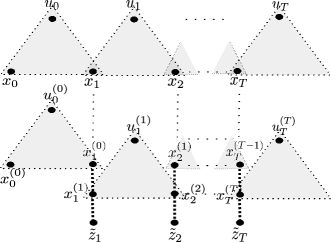
Figure 1: The idea of the time splitting algorithm. Whenever the dynamics introduce a coupling of variables, they are decoupled via a slack variable $\tilde{z}_{t}=x_{t}^{t}=x_{t}^{(t-1)}$.

II-B The time-splitting algorithm

In order to use a more compact formulation, we will denote the decision variables in (2) corresponding to each subproblem using

$$\tilde{x}_{t}=(x_{t}^{(t)},u_{t}^{(t)},x_{t+1}^{(t)}),$$ (3)

where $\tilde{x}_{t}\in{\mbox{\bf R}}^{2n+m}$. We also introduce dual variables to deal with the consensus equality constraints:

• $\tilde{w}_{t}$ associated with $x_{t}^{(t)}=\tilde{z}_{t},\quad t=1,\ldots,N$ and
  

• $\tilde{v}_{t}$ associated with $x_{t}^{(t-1)}=\tilde{z}_{t},\quad t=1,\ldots,N$.

In order to rewrite the finite-time optimal control problem in a more compact form, we define the following matrices:

$$P_{t} = \left[\begin{array}[]{ccc}Q_{t}&0&0\\ 0&R_{t}&0\\ 0&0&0\end{array}\right]\in{\mbox{\bf R}}^{(2n+m)\times(2n+m)},$$ (4d)

$$F_{t} = \left[\begin{array}[]{ccc}-A_{t}&-B_{t}&I\end{array}\right]\in{\mbox{\bf R}}^{n\times(2n+m)},$$ (4f)

$$G_{0} = \left[\begin{array}[]{ccc}I&0&0\end{array}\right]\in{\mbox{\bf R}}^{n\times(2n+m)},$$ (4h)

$$G_{1} = \left[\begin{array}[]{ccc}0&0&I\end{array}\right]\in{\mbox{\bf R}}^{n\times(2n+m)}.$$ (4j)

We use the ALternating Direction Method of Multipliers (ADMM) [13, 14] in order to arrive at a solution approach that is amenable to parallel implementation. The updates involved in the ADMM algorithm include forming the augmented Lagrangian of the problem and minimizing over the primal variables $\tilde{x}_{t},\;t=0,\ldots,N$ and $\tilde{z}_{t},\;t=1,\ldots,N$, followed by updating the dual variables $\tilde{w}_{t}$ and $\tilde{v}_{t},\;t=1,\ldots,N$. The three main steps of the algorithm are performed in an iterative fashion and are described next in detail. We use $k$ to denote the algorithm’s loop counter. The termination criterion based on primal and dual tolerances are provided and the analytic derivation of the formulas in each step is presented in the Appendix.

Step 1: Solving $N+1$ QP subproblems for the primal variables in $\tilde{x}_{t}$
Minimization of the augmented Lagrangian over the primal variables $\tilde{x}_{t}$ results in $N+1$ stage-wise quadratic programs (QPs):

• For the subproblem associated with the time instant $t=0$, we need to solve

  $$\begin{array}[]{llll}&\mbox{minimize}&&(1/2)\tilde{x}_{0}^{T}P_{0}\tilde{x}_{0}-\rho\tilde{v}_{1}^{kT}(G_{1}\tilde{x}_{0}-\tilde{z}_{1}^{k})\\ &&&+(\rho/2)\|G_{1}\tilde{x}_{0}-\tilde{z}_{1}^{k}\|_{2}^{2}\\ &\mbox{subject to}&&\tilde{x}_{0}\in\mathcal{C}_{0}\\ &&&G_{0}\tilde{x}_{0}=x_{\mathrm{init}}\\ &&&F_{0}\tilde{x}_{0}=c_{0}\end{array}$$ (5)

  with variable $\tilde{x}_{0}$.

• Similarly, we need to solve the following QPs for all the other groups of variables $\tilde{x}_{t},\;t=1,\ldots,N-1$:

  $$\begin{array}[]{llll}&\mbox{minimize}&&(1/2)\tilde{x}_{t}^{T}P_{t}\tilde{x}_{t}-\rho\tilde{v}_{t+1}^{kT}(G_{1}\tilde{x}_{t}-\tilde{z}_{t+1}^{k})\\ &&&+(\rho/2)\|G_{1}\tilde{x}_{t}-\tilde{z}_{t+1}^{k}\|_{2}^{2}\\ &&&-\rho\tilde{w}_{t}^{kT}(G_{0}\tilde{x}_{t}-\tilde{z}_{t}^{k})\\ &&&+(\rho/2)\|G_{0}\tilde{x}_{t}-\tilde{z}_{t}^{k}\|_{2}^{2}\\ &\mbox{subject to}&&\tilde{x}_{t}\in\mathcal{C}_{t}\\ &&&F_{t}\tilde{x}_{t}=c_{t}\end{array}$$ (6)

• For the subproblem associated with the final time instant $t=N$, we need to solve

  $$\begin{array}[]{llll}&\mbox{minimize}&&(1/2)\tilde{x}_{N}^{T}P_{N}\tilde{x}_{N}-\rho\tilde{w}_{N}^{kT}(G_{0}\tilde{x}_{N}-\tilde{z}_{N}^{k})\\ &&&+(\rho/2)\|G_{0}\tilde{x}_{N}-\tilde{z}_{N}^{k}\|_{2}^{2}\\ &\mbox{subject to}&&\tilde{x}_{N}\in\mathcal{C}_{N}\end{array}$$ (7)

  with variable $\tilde{x}_{N}$.

The polyhedral sets $\mathcal{C}_{t},\;t=0,\ldots,N$ are defined as

$$\mathcal{C}_{t}=\mathcal{X}_{t}\times\mathcal{U}_{t}\times\mathcal{X}_{t+1}\subseteq{\mbox{\bf R}}^{2n+m}$$ (8)

and the variable $\rho>0$ is a parameter of the algorithm.

Remark 1

Notice that for the time instant $N$ the decision variables of the QP actually simplify to $\tilde{x}_{N}=x_{N}$ and $\mathcal{C}_{N}=\mathcal{X}_{N}$, but we keep the same notation for simplicity (and without loss of generality).

Step 2: Averaging
The update of the ‘global’ primal variables $\tilde{z}_{t},\;t=1,\ldots,N$ is derived from a simple quadratic minimization problem, the solution of which turns out to be an average of the predicted ($x_{t}^{(t-1)}$) and current ($x_{t}^{(t)}$) state

$$\tilde{z}_{t}^{k+1}=\frac{G_{0}\tilde{x}_{t}^{k+1}+G_{1}\tilde{x}_{t-1}^{k+1}}{2},\quad t=1,\ldots,N.$$ (9)

This intuitively makes sense, since the global variable can be obtained by collecting the local (primal) ones and computing the best estimate based on their values.

Step 3: Dual update
The dual updates can be expressed as

$$\tilde{w}_{t}^{k+1} = \tilde{w}_{t}^{k}-G_{0}\tilde{x}_{t}^{k+1}+\tilde{z}_{t}^{k+1},$$ (10a)

$$\tilde{v}_{t}^{k+1} = \tilde{v}_{t}^{k}-G_{1}\tilde{x}_{t-1}^{k+1}+\tilde{z}_{t}^{k+1},\quad t=1,\ldots,N.$$ (10b)

Termination criterion
The algorithm terminates when a set of primal and dual residuals are bounded by a specified threshold (primal and dual tolerances); see [12, §3.2]. The primal and dual residuals for the time-splitting algorithm are defined as

$$r^{k}=A_{\mathrm{res}}x_{\mathrm{pri}}^{k}+B_{\mathrm{res}}z_{\mathrm{pri}}^{k},$$ (11)

and

$$s^{k}=-\rho A_{\mathrm{res}}^{T}B_{\mathrm{res}}(z_{\mathrm{pri}}^{k}-z_{\mathrm{pri}}^{k-1}),$$ (12)

respectively.

The termination criterion is activated when

$$\|r^{k}\|_{2}\leq\epsilon^{\mathrm{pri}},\quad\|s^{k}\|_{2}\leq\epsilon^{\mathrm{dual}},$$

where the tolerances $\epsilon^{\mathrm{pri}}$ and $\epsilon^{\mathrm{dual}}$ are defined as follows:

$$\epsilon^{\mathrm{pri}} = \epsilon^{\mathrm{abs}}\sqrt{N2n}$$ (13a)

$$+\epsilon^{\mathrm{rel}}\max\{\|A_{\mathrm{res}}x_{\mathrm{pri}}\|_{2},\|B_{\mathrm{res}}z_{\mathrm{pri}}\|_{2},\|c_{\mathrm{res}}\|_{2}\}$$ (13b)

$$\epsilon^{\mathrm{dual}} = \epsilon^{\mathrm{abs}}\sqrt{(2n+m)(N+1)}+\epsilon^{\mathrm{rel}}\|A_{\mathrm{res}}^{T}v_{\mathrm{dual}}\|_{2}$$ (13c)

and we defined the vectors

$$x_{\mathrm{pri}}=\left[\begin{array}[]{c}\tilde{x}_{0}\\ \tilde{x}_{1}\\ \vdots\\ \tilde{x}_{N}\end{array}\right],\qquad z_{\mathrm{pri}}=\left[\begin{array}[]{c}\tilde{z}_{1}\\ \tilde{z}_{2}\\ \vdots\\ \tilde{z}_{N}\end{array}\right],\qquad v_{\mathrm{dual}}=\left[\begin{array}[]{c}\tilde{v}_{1}\\ \tilde{w}_{1}\\ \tilde{v}_{2}\\ \vdots\\ \tilde{v}_{N}\\ \tilde{w}_{N}\end{array}\right].$$

The residual matrices $A_{\mathrm{res}}$ and $B_{\mathrm{res}}$ and the residual vector $c_{\mathrm{res}}$ are

$$A_{\mathrm{res}}=\left[\begin{array}[]{cccccc}G_{1}&0&0&\cdots&0&0\\ 0&G_{0}&0&\cdots&0&0\\ 0&G_{1}&0&\cdots&0&0\\ 0&0&G_{0}&\cdots&0&0\\ 0&0&G_{1}&\cdots&0&0\\ \vdots&\vdots&\vdots&\ddots&\vdots&\vdots\\ 0&0&0&\cdots&G_{0}&0\\ 0&0&0&\cdots&G_{1}&0\\ 0&0&0&\cdots&0&G_{0}\end{array}\right]\in{\mbox{\bf R}}^{T2n\times(N+1)(2n+m)},$$

$$B_{\mathrm{res}}=\left[\begin{array}[]{cccc}-I&0&\cdots&0\\ -I&0&\cdots&0\\ 0&-I&\cdots&0\\ 0&-I&\cdots&0\\ \vdots&\vdots&\ddots&\vdots\\ 0&0&\cdots&-I\\ 0&0&\cdots&-I\\ \end{array}\right]\in{\mbox{\bf R}}^{N2n\times Nn},$$

and $c_{\mathrm{res}}\in{\mbox{\bf R}}^{N2n}$ is zero.

The three update steps described above are fully parallelizable at each iteration $k$. Assuming $N+1$ processors are available, then processor $\Pi_{t}$ would need to execute the following actions for $t=0,\ldots,N-1$:

1. Receive the estimate $\tilde{z}_{t+1}^{k}$ $\tilde{v}_{t+1}^{k}$ and from neighboring processor $\Pi_{t+1}$ (6).

2. Compute $\tilde{x}_{t}^{k+1}$.

3. Receive the estimate $\tilde{x}_{t-1}^{k+1}$ from neighboring processor $\Pi_{t-1}$ and compute $\tilde{z}_{t}^{k+1}$ (9).

4. Compute $\tilde{w}_{t}^{k+1}$ and $\tilde{v}_{t}^{k+1}$ (10).

5. Communicate $\tilde{x}_{t}^{k+1}$ to processors $\Pi_{t-1}$ and $\Pi_{t+1}$, and $\tilde{z}_{t}^{k+1}$, $\tilde{v}_{t}^{k+1}$ to processor $\Pi_{t-1}$.

The above scheme suggests that each processor $\Pi_{t},\;t=1,\ldots,N-1$ interacts with the two neighboring processors $\Pi_{t-1}$ and $\Pi_{t+1}$. Processors $\Pi_{0}$ and $\Pi_{N}$ communicate only with processors $\Pi_{1}$ and $\Pi_{N-1}$, respectively. After updating all variables, a gather operation follows in order to compute the residuals and check the termination criterion.

III THREE-SET SPLITTING QP SOLVER

III-A Motivation

The time-splitting algorithm presented in the previous section decomposes the centralized finite-time optimal control problem so that it can be solved using multiple parallel processors. However, the updates for the primal variables $\tilde{x}_{t},\;t=0,\ldots,N$ given in (5), (6) and (7) involve solving a QP at each iteration of the algorithm. Even though several fast interior point solvers exist for this purpose (see e.g., [15]), these are mostly suitable for only a limited number of variables. Although recently more computationally efficient schemes that scale better with the problem size have been developed, they are restricted to cases where simple box constraints are considered [16, 8, 10]. In order to achieve fast computations in an embedded control environment, other generic solution methods would be preferred.

In this section we propose an alternative scheme for solving the QPs with general polyhedral constraints that arise in the previous section. We propose to perform yet another type of splitting approach, which splits the state-input variables of the QP in three sets. One set involves the variables that appear in the objective function, another set includes those that appear in the dynamics equality constraints, and the last set contains variables from the inequality constraints. In this way, we solve three simpler subproblems instead of the single general QP. Since several variables are shared among the subproblems, their solutions must be in consensus again to ensure consistency.

An important element of the proposed method is the introduction of an extra slack variable, which allows to get an analytic solution for the subproblem associated with the inequality constraints. Using this variable, the projection on any polyhedral set can be practically rewritten as a projection onto the nonnegative orthant. Besides this feature, the proposed splitting exploits structure in the resulting matrices and thus modern numerical linear algebra methods can be employed for speeding up the computations.

III-B Problem setup

We consider a QP of the form

$$\begin{array}[]{ll}\mbox{minimize}&\frac{1}{2}x^{T}Mx+q^{T}x+r\\ \mbox{subject to}&Ax=b\\ &Hx\preceq h,\end{array}$$ (14)

with decision variable $x\in{\mbox{\bf R}}^{n}$, where $M\in S_{+}^{n}$, $q\in{\mbox{\bf R}}^{n}$, $r\in{\mbox{\bf R}}$, $A\in{\mbox{\bf R}}^{m\times n}$, $b\in{\mbox{\bf R}}^{m}$, $H\in{\mbox{\bf R}}^{p\times n}$, $h\in{\mbox{\bf R}}^{p}$ and $S_{+}^{n}$ is the cone of positive semidefinite matrices of dimension $n$.

In order to apply a variable splitting idea for this problem we first replicate all variables appearing in (14) three times, introducing three different sets for which we must ensure consensus. Furthermore, we use a slack variable to remove the polyhedral constraint and transform it into a projection operation onto the nonnegative orthant. We define the following sets of variables:

• First set - objective: $x^{\textrm{I}}$
  

• Second set - equality constraints: $x^{\textrm{II}}$
  

• Third set - inequality constraints: $x^{\textrm{III}}$
  

• First global variable: $z=x^{\textrm{I}}=x^{\textrm{II}}=x^{\textrm{III}}$
  

• Second global variable: $y=h-Hx^{(\textrm{III})}$
  

• First set of dual variables: $\tilde{z}^{\textrm{I}},\tilde{z}^{\textrm{II}},\tilde{z}^{\textrm{III}}$ associated with $z=x^{\textrm{I}}=x^{\textrm{II}}=x^{\textrm{III}}$, respectively.
  

• Second set of dual variables: $\tilde{y}$ associated with $y=h-Hx^{\textrm{III}}$

Using the above sets of variables problem (14) can be restated in the equivalent form

minimize $$\frac{1}{2}x^{\textrm{I}T}Mx^{\textrm{I}}+q^{T}x^{\textrm{I}}+r$$ (15a)

subject to $$Ax^{\textrm{II}}=b$$ (15b)

$$y=h-Hx^{\textrm{III}},\quad y\succeq 0$$ (15c)

$$x^{\textrm{I}}=x^{\textrm{II}}=x^{\textrm{III}}=z,$$ (15d)

with variables $x^{\textrm{I}},x^{\textrm{II}},x^{\textrm{III}},z\in{\mbox{\bf R}}^{n},y\in{\mbox{\bf R}}^{p}$. The dual variables are of dimensions $\tilde{z}\in{\mbox{\bf R}}^{n},\tilde{y}\in{\mbox{\bf R}}^{p}$.

III-C The proposed three-set splitting algorithm

The proposed algorithm consists of iterative updates to the three ADMM steps similarly to the case of the time-splitting approach in Section II-B, namely one for the (local) primal variables $x^{\textrm{I}},x^{\textrm{II}},x^{\textrm{III}}$, one for the (global) primal variables $z$ and $y$ and one for the dual variables $\tilde{z}^{\textrm{I}},\tilde{z}^{\textrm{II}},\tilde{z}^{\textrm{III}}$ and $\tilde{y}$. We provide the algorithm’s steps below along with some clarifying comments. The analytic derivations are presented in the Appendix.

Step 1: Solving three subproblems for the primal variables $x^{\textrm{I}},x^{\textrm{II}},x^{\textrm{III}}$
In all three cases we have to solve simple, unconstrained QPs. The updates are:

$$\left(x^{\textrm{I}}\right)^{k+1}=(M+\rho I)^{-1}(\rho(z^{k}+\left(\tilde{z}^{\textrm{I}}\right)^{k})-q)$$ (16)

$$\left[\begin{array}[]{cc}\rho I&A^{T}\\ A&0\end{array}\right]\left[\begin{array}[]{c}\left(x^{\textrm{II}}\right)^{k+1}\\ \nu\end{array}\right]=\left[\begin{array}[]{c}\rho(z^{k}+\left(\tilde{z}^{\textrm{II}}\right)^{k})\\ b\end{array}\right],$$ (17)

where $\nu$ is the dual variable associated with the equality constraint $Ax^{\textrm{II}}=b$, and

$$\left(x^{\textrm{III}}\right)^{k+1} = (H^{T}H+I)^{-1}\Big{(}H^{T}(h-\tilde{y}^{k}-y^{k})+$$ (18)

$$z^{k}+\left(\tilde{z}^{\textrm{III}}\right)^{k}\Big{)}{}.$$

The matrices $M+\rho I$ and $H^{T}H+I$ are symmetric positive definite due to the regularization terms. This means that, instead of directly inverting the matrices, we can save computational effort by taking the Cholesky factorization, i.e., write the matrix as a product of a lower triangular matrix and its transpose (see, e.g., [17]). Furthermore, the matrix $\left[\begin{array}[]{cc}\rho I&A^{T}\\ A&0\end{array}\right]$ is a KKT matrix and $\rho I\succ 0$. Hence we can exploit its structure and use block elimination to solve the KKT system (see [18, App. C]). The resulting matrices can be pre-factorized and then used in every solve step. The right-hand sides are the only parts that change in the update loop.

Step 2: Averaging and projection
The update for $z$ is

$$z^{k+1}=\frac{1}{3}\sum_{i=\textrm{I}}^{\textrm{III}}\left(x^{i}\right)^{k+1},$$ (19)

while for $y$ it is

$$y^{k+1}=\left(h-H\left(x_{t}^{\textrm{III}}\right)^{k+1}-\tilde{y}^{k}\right)_{+}.$$ (20)

The $z$-update is an averaging over the three sets of the primal variables $x^{\textrm{I}},x^{\textrm{II}},x^{\textrm{III}}$, while the $y$-update is the solution of a proximal minimization problem (see Appendix), resulting in a projection onto the nonnegative orthant, denoted by $(\cdot)_{+}$.

Step 3: Dual update
The update for the dual variables $\tilde{z}^{i}$ is

$$\left(\tilde{z}^{i}\right)^{k+1}=\left(\tilde{z}^{i}\right)^{k}-\left(x^{i}\right)^{k+1}+z^{k+1},\quad i=\textrm{I},\textrm{II},\textrm{III}.$$ (21)

Similarly, the update for $\tilde{y}$ is

$$\tilde{y}^{k+1}=\tilde{y}^{k}+y^{k+1}-h+H\left(x^{\textrm{III}}\right)^{k+1}.$$ (22)

Termination criterion
The primal and dual tolerances $\epsilon^{\mathrm{pri}}$ and $\epsilon^{\mathrm{dual}}$ are given by

$$\begin{array}[]{rcl}\epsilon^{\mathrm{pri}}&=&\epsilon^{\mathrm{abs}}\sqrt{3n+p}+\epsilon^{\mathrm{rel}}\max\{\|A_{\mathrm{res}}(x^{\textrm{I}},x^{\textrm{II}},x^{\textrm{III}})\|_{2},\\ &&\|B_{\mathrm{res}}(z,y)\|_{2},\|c_{\mathrm{res}}\|_{2}\}\\ \epsilon^{\mathrm{dual}}&=&\epsilon^{\mathrm{abs}}\sqrt{3n}+\epsilon^{\mathrm{rel}}\|A_{\mathrm{res}}^{T}(\tilde{z}^{\textrm{I}},\tilde{z}^{\textrm{II}},\tilde{z}^{\textrm{III}},\tilde{y})\|_{2}.\end{array},$$ (23)

The residual matrices $A_{\mathrm{res}}$ and $B_{\mathrm{res}}$ and the residual vector $c_{\mathrm{res}}$ are

$$A_{\mathrm{res}}=\left[\begin{array}[]{ccc}I&0&0\\ 0&I&0\\ 0&0&I\\ 0&0&H\end{array}\right],\quad B_{\mathrm{res}}=\left[\begin{array}[]{cc}-I&0\\ -I&0\\ -I&0\\ 0&I\end{array}\right],$$

and

$$c_{\mathrm{res}}=(0,0,0,h),$$

where $A_{\mathrm{res}}\in{\mbox{\bf R}}^{(3n+p)\times 3n}$, $B_{\mathrm{res}}\in{\mbox{\bf R}}^{(3n+p)\times(n+p)}$ and $c_{\mathrm{res}}\in{\mbox{\bf R}}^{3n+p}$.

Remark 2

For the QP corresponding to the last sample time $t=N$ (7), the algorithm simplifies to splitting into two sets (objective and inequality constraints), since there are no dynamics equality constraints. The updates and residuals follow directly from the more generic case presented above.

IV HIERARCHICAL TIME-SPLITTING OPTIMAL CONTROL

It is a natural idea to combine the two splitting algorithms (time-splitting and three-set splitting) that were introduced in the preceding two sections in order to speed up the solution of the finite-time optimal control problem (1). This can be accomplished via a nested decomposition scheme, where we employ the three-set splitting algorithm to solve the QPs (5), (6) and (7) appearing in Step 1 of the time-splitting algorithm. The idea is graphically depicted in Figure 2.

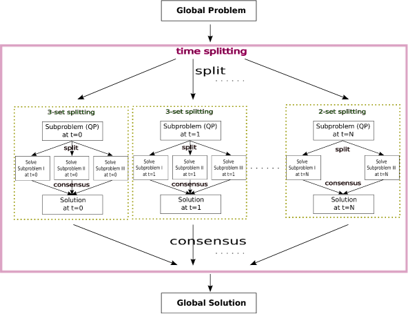
Figure 2: Structural representation of the hierarchical time-splitting solution approach to the finite-time optimal control problem. The outer subproblems at $t=0,1,\ldots,N$ refer to (5), (6) and (7), respectively. The solutions of the nested subproblems enumerated by I, II and III correspond to (16), (17) and (18). Notice that only 2 subproblems have to be solved for the last time instant $t=N$.

If we rewrite the generalized inequality constraints appearing in the problem formulation as

$$(x_{t}^{(t)},u_{t}^{(t)})\in\mathcal{C}_{t}\;\Leftrightarrow\;H_{t}\tilde{x}_{t}\preceq h_{t},\quad t=0,\ldots,N,$$ (24)

then the QPs can be written in the form described by (14), where we consider the following relations:

• For $\tilde{x}_{0}$, Eq. $(\ref{eq:time_split_x0})$:
  

  $$M = P_{0}+\rho G_{1}^{T}G_{1},$$

  $$q = -\rho G_{1}^{T}(\tilde{z}_{1}+\tilde{v}_{1}),$$

  $$r = (\rho/2)\tilde{z}_{1}^{T}\tilde{z}_{1}+\rho\tilde{v}_{1}^{T}\tilde{z}_{1},$$

  $$A = (G_{0},F_{0}),$$

  $$b = (x_{\mathrm{init}},c_{0}),$$

  $$H = \left[\begin{array}[]{cc}H_{0}&0\end{array}\right],$$

  $$h = h_{0}.$$

• For $\tilde{x}_{t},\;t=1,\ldots,N-1$, Eq. $(\ref{eq:time_split_xt})$:
  

  $$M = P_{t}+\rho(G_{0}^{T}G_{0}+G_{1}^{T}G_{1}),$$

  $$q = -\rho(G_{0}^{T}(\tilde{z}_{t}+\tilde{w}_{t})+G_{1}^{T}(\tilde{z}_{t+1}+\tilde{v}_{t+1})),$$

  $$r = (\rho/2)(\tilde{z}_{t+1}^{T}\tilde{z}_{t+1}+\tilde{z}_{t}^{T}\tilde{z}_{t})+\rho(\tilde{v}_{t+1}^{T}\tilde{z}_{t+1}+\tilde{w}_{t}^{T}\tilde{z}_{t}),$$

  $$A = F_{t},$$

  $$b = c_{t},$$

  $$H = \left[\begin{array}[]{cc}H_{t}&0\end{array}\right],$$

  $$h = h_{t}.$$

• For $\tilde{x}_{N}$, Eq. $(\ref{eq:time_split_xT})$:
  

  $$M = P_{N}+\rho G_{0}^{T}G_{0},$$

  $$q = -\rho G_{0}^{T}(\tilde{z}_{N}+\tilde{w}_{N}),$$

  $$r = (\rho/2)\tilde{z}_{N}^{T}\tilde{z}_{N}+\rho\tilde{w}_{N}^{T}\tilde{z}_{N},$$

  $$A = 0,$$

  $$b = 0,$$

  $$H = \left[\begin{array}[]{cc}H_{N}&0\end{array}\right],$$

  $$h = h_{N}.$$

For each iteration of the time-splitting algorithm, the three-set splitting algorithm runs in an inner loop until it converges. The quality of this convergence, i.e., the choice of the primal and dual tolerances of the inner loop (23) will affect the quality of the global solution.

A method that enables substantial speedup of the algorithm is warm starting. Since the three-set splitting algorithm will run for every iteration of the time-splitting algorithm, we can warm-start each QP with its previous solution. In this way, we can achieve a significant reduction in the number of iterations needed for the convergence of the inner loop.

V NUMERICAL RESULTS

We consider three, randomly generated, numerical examples to illustrate the performance of the algorithm. The examples vary in terms of the number of decision variables involved. The systems considered are linear and time-invariant. We impose constraints on the difference between two consecutive states at each time instant of the form

$$x_{t,i}-x_{t,i-1}\leq dx,$$

where $x_{ti}\in{\mbox{\bf R}},\;i=1,\ldots,n,\;,t=0,\ldots,N$ and box constraints on the inputs, i.e.,

$$\|u_{t}\|_{\infty}\leq u_{\mathrm{max}},\;t=0,\ldots,N-1.$$

By adjusting the level of the disturbance $c_{t}$ in several time instances, we ensure activation of the constraints along the horizon.

For the simulations, we used an Intel Core i7 processor running at 1.7 GHz. We compared a C-implementation of our algorithm with using CVX [19], a parser-solver that uses SDPT3 [20]. For our method, the tolerances for both the outer and inner algorithms are set as $\epsilon^{\mathrm{pri}}=10^{-4}$ and $\epsilon^{\mathrm{dual}}=10^{-3}$. The parameter $\rho$ was set after some simple tuning. The linear systems appearing in (16), (17) and (18) were solved by first factorizing the matrices off-line, using Tim Davis’s sparse package [21, 22, 23] (see also [8]). The finite-time optimal control problem was solved only once and all the primal and dual variables were initialized at zero. However, the inner algorithm was warm-started at every iteration of the outer algorithm to the values acquired from the previous iteration. No relaxation or any other variance of the iterations was used. The numerical results are summarized in Table I, where the computation times are reported in ms.

	small	medium	large
states $n$	10	20	50
inputs $m$	10	10	40
horizon length $N$	10	30	60
total variables	220	900	5400
$\rho$	15	25	50
active box constraints	5	6	20
active inequality constraints	2	2	4
CVX solve time	2430	3529	19420
factorization time	3.18	9.5	30
	Tolerance $10^{-4}$
3-set (average) iterations	21.80	17	15.95
3-set (average) solve time	0.75	1.38	9.15
time-split. iterations	250	241	389
time-split. solve time (single thread)	1880	10023	215888
time-split. solve time ($N$ threads∗)	188	334.1	3598
	Tolerance $10^{-3}$
3-set (average) iterations	13.14	13.27	12.32
3-set (average) solve time	0.49	1.18	7.34
time-split. iterations	156	128	224
time-split. solve time (single thread)	780	4304	99525
time-split. solve time ($N$ threads∗)	78	143.47	1659
∗ estimated parallel computation times

TABLE I: Hierarchical time-splitting optimal control: computational time results for different size problems.

We can observe that, in the case of the small system, even when solving the problem on a single thread, the computation times are smaller than those of CVX. As the problem scales, the computations have to be parallelized in order to gain a significant advantage. More specifically, we expect the following speedup factors: 13 and 31 times faster in the case of the small problem (for the corresponding tolerances set to $10^{-4}$ and $10^{-3}$ respectively). For the medium-sized problem the speedups are by a factor of 10.5 and 24.6, and a factor of 5.4 and 11.7 for the large-scale problem, respectively.

In addition, we could observe that the factorization times are negligible in all cases, since the matrices being factorized are not large. Concerning the three-set splitting algorithm, only the average computational times are indicated over all iterations required to solve the problem.

VI CONCLUSIONS

In this paper, we proposed an algorithm that solves a centralized convex finite-time optimal control problem making use of operator splitting methods, and, more specifically, the Alternating Direction Method of Multipliers. The initial problem is split into as many subproblems as the horizon length, which then can be solved in parallel.

The resulting algorithm is composed of three steps, including one where several QPs have to be solved. In this respect, we proposed another method, based again on operator splitting, that is applicable to QPs of any size, involving polyhedral constraints. This algorithm exploits the structure of the problem, leading to fast solutions.

The combination of the proposed algorithms results in a nested decomposition scheme for solving the aforementioned finite-time optimal control problems over several parallel processors.

Our numerical experiments suggest that the proposed hierarchical decomposition approach provides significant speed-up in computational time required for medium accuracy solutions for the class of problems considered. In our future work we intend to perform an even more extensive comparison with very recent tailor-made computational tools, and implement the algorithm on a parallel computing platform to obtain more accurate and representative computational time measurements.

APPENDIX

Derivation of the time-splitting algorithm updates

We solve the relaxed version of the convex optimization problem (2) by formulating the augmented Lagrangian with respect to the additional equality constraints, using the matrices and vectors defined in (3) and (4). The augmented Lagrangian can be written as

$$L_{\rho}(\tilde{x}_{t},x_{\mathrm{init}},\tilde{w}_{t},\tilde{y}_{t},\tilde{z}_{t},\nu_{t}):=$$ (28)

$$~{}~{}~{}~{}~{}~{}\sum_{t=0}^{N}\left(\frac{1}{2}\tilde{x}_{t}^{T}P\tilde{x}_{t}+I_{\mathcal{C}_{t}}(\tilde{x}_{t})\right)+\nu_{0}^{T}(\tilde{x}_{0}-x_{\mathrm{init}})$$

$$~{}~{}~{}~{}~{}~{}+\sum_{t=0}^{N-1}\nu_{t+1}^{T}(F\tilde{x}_{t}-c_{t})$$

$$~{}~{}~{}~{}~{}~{}+\sum_{t=0}^{N-1}\Big{(}-\rho\tilde{v}_{t+1}^{T}(G_{1}\tilde{x}_{t}-\tilde{z}_{t+1})+\frac{\rho}{2}\|G_{1}\tilde{x}_{t}-\tilde{z}_{t+1}\|_{2}^{2}\Big{)}$$

$$~{}~{}~{}~{}~{}~{}+\sum_{t=1}^{N}\Big{(}-\rho\tilde{w}_{t}^{T}(G_{0}\tilde{x}_{t}-\tilde{z}_{t})+\frac{\rho}{2}\|G_{0}\tilde{x}_{t}-\tilde{z}_{t}\|_{2}^{2}\Big{)}.$$

The dual variables $\nu_{t}\in{\mbox{\bf R}}^{n},\;t=0,\ldots,N$ are associated with the equality constraints. We define the indicator function for the polyhedral set $\mathcal{C}_{t}\subset{\mbox{\bf R}}^{2n+m}$ as

$$I_{\mathcal{C}_{t}}(\tilde{x}_{t})=\left\{\begin{array}[]{ll}0&\tilde{x}_{t}\in\mathcal{C}_{t}\\ \infty&\mbox{otherwise}.\end{array}\right.$$

The augmented Lagrangian is minimized (and maximized) over the primal (and dual) variables in an iterative manner, for each iteration of the algorithm.

By treating the dynamics and inequality constraints as explicit and minimizing with respect to $\tilde{x}_{t},\;t=0,\ldots,N$, we end up with the stage-wise QPs (5), (6), (7).

The update of $\tilde{z}_{t}$ is given by solving

$$\tilde{z}_{t}^{k+1} = \mathop{\rm argmin}_{\tilde{z}_{t}}\Big{(}-\rho\tilde{v}_{t}^{kT}(G_{1}\tilde{x}_{t-1}^{k+1}-\tilde{z}_{t})$$

$$+ \frac{\rho}{2}\|G_{1}\tilde{x}_{t-1}^{k+1}-\tilde{z}_{t}\|_{2}^{2}$$

$$- \rho\tilde{w}_{t}^{kT}(G_{0}\tilde{x}_{t}^{k+1}-\tilde{z}_{t})+\frac{\rho}{2}\|G_{0}\tilde{x}_{t}^{k+1}-\tilde{z}_{t}\|_{2}^{2}\Big{)}$$

$$= \mathop{\rm argmin}_{\tilde{z}_{t}}\Big{(}\frac{\rho}{2}\|\tilde{z}_{t}-G_{1}\tilde{x}_{t-1}^{k+1}+\tilde{v}_{t}^{k}\|_{2}^{2}-\frac{\rho}{2}\|\tilde{v}_{t}^{k}\|_{2}^{2}$$

$$+ \frac{\rho}{2}\|\tilde{z}_{t}-G_{0}\tilde{x}_{t}^{k+1}+\tilde{w}_{t}^{k}\|_{2}^{2}-\frac{\rho}{2}\|\tilde{w}_{t}^{k}\|_{2}^{2}\Big{)}\Rightarrow$$

$$\tilde{z}_{t}^{k+1} = \frac{G_{0}\tilde{x}_{t}^{k+1}+G_{1}\tilde{x}_{t-1}^{k+1}-\tilde{v}_{t}^{k}-\tilde{w}_{t}^{k}}{2},\quad t=1,\ldots,N{}$$ (29)

Rearranging the terms in (28) and completing the squares as before, the dual updates for $\tilde{w}_{t}$ and $\tilde{v}_{t}$ result by solving

$$\tilde{w}_{t}^{k+1} = \mathop{\rm argmax}_{\tilde{w}_{t}}\left(\frac{\rho}{2}\|\tilde{w}_{t}-G_{0}\tilde{x}_{t}^{k+1}+\tilde{z}_{t}^{k+1}\|_{2}^{2}-\frac{\rho}{2}\|\tilde{w}_{t}\|_{2}^{2}\right),$$

$$\tilde{v}_{t}^{k+1} = \mathop{\rm argmax}_{\tilde{v}_{t}}\left(\frac{\rho}{2}\|\tilde{v}_{t}-G_{1}\tilde{x}_{t-1}^{k+1}+\tilde{z}_{t}^{k+1}\|_{2}^{2}-\frac{\rho}{2}\|\tilde{v}_{t}\|_{2}^{2}\right)$$

The dual updates are

$$\tilde{w}_{t}^{k+1} = \tilde{w}_{t}^{k}-G_{0}\tilde{x}_{t}^{k+1}+\tilde{z}_{t}^{k+1}{},$$ (30)

$$\tilde{v}_{t}^{k+1} = \tilde{v}_{t}^{k}-G_{1}\tilde{x}_{t-1}^{k+1}+\tilde{z}_{t}^{k+1},\quad t=1,\ldots,T.{}$$ (31)

Substituting (30) and (31) into (29) results in $\tilde{w}_{t}^{k+1}+\tilde{v}_{t}^{k+1}=0$, for all $t$. Hence $\tilde{z}_{t}^{k+1}$ can be simplified to

$$\tilde{z}_{t}^{k+1}=\frac{G_{0}\tilde{x}_{t}^{k+1}+G_{1}\tilde{x}_{t-1}^{k+1}}{2},\quad t=1,\ldots,N.$$

This result shows that $\tilde{z}_{t}$ is the variable that enforces consensus upon $x_{t}^{(t)}$ and $x_{t}^{(t-1)}$, the value of which is the average of the two.

Derivation of the three-set splitting algorithm updates

The augmented Lagrangian for (15) can be written as

$$L_{\rho}(x,z,y,\tilde{z},\tilde{y},\nu):=$$ (32)

$$~{}~{}~{}~{}~{}~{}\frac{1}{2}x^{\textrm{I}T}Mx^{\textrm{I}}+q^{T}x^{\textrm{I}}+r+\nu^{T}(\tilde{A}x^{\textrm{II}}-\tilde{b})$$

$$~{}~{}~{}~{}~{}~{}-\rho\sum_{i=\textrm{I}}^{\textrm{III}}\tilde{z}^{iT}(x^{i}-z)+\frac{\rho}{2}\sum_{i=\textrm{I}}^{\textrm{III}}\|x^{i}-z\|_{2}^{2}$$

$$~{}~{}~{}~{}~{}~{}-\rho\tilde{y}^{T}(\tilde{h}-\tilde{H}x^{\textrm{III}}-y)+\frac{\rho}{2}\|\tilde{h}-\tilde{H}x^{\textrm{III}}-y\|_{2}^{2}+I_{\{y\in{\mbox{\bf R}}_{+}^{p}\}}.$$

As before, the dual variable $\nu$ is associated with the equality constraints. We define the indicator function of the nonnegative orthant for a variable $x\in{\mbox{\bf R}}$ as

$$I_{\{x\in{\mbox{\bf R}}_{+}\}}=x_{+}=\left\{\begin{array}[]{ll}x&x\geq 0\\ \infty&\mbox{otherwise}.\end{array}\right.$$

The function applies componentwise for vector variables.

The augmented Lagrangian is a smooth, quadratic function with respect to the variables $x^{\textrm{I}},x^{\textrm{II}},x^{\textrm{III}}$, hence the updates can be derived from taking the gradient equal to zero. This yields the solutions (16), (17) and (18).

Grouping the terms that involve $z$ from (32) we obtain

$$z^{k+1} = \mathop{\rm argmin}_{z}\left(\sum_{i=\textrm{I}}^{\textrm{III}}\frac{\rho}{2}\|z-\left(x^{i}\right)^{k+1}+\left(\tilde{z}^{i}\right)^{k}\|^{2}\right)\Rightarrow$$

$$z^{k+1} = \frac{1}{3}\sum_{i=\textrm{I}}^{\textrm{III}}\left(\left(x^{i}\right)^{k+1}-\left(\tilde{z}^{i}\right)^{k}\right).{}$$ (33)

Maximizing (32) over $\tilde{z}^{i},i=\textrm{I},\textrm{II},\textrm{III}$ results in

$$\left(\tilde{z}^{i}\right)^{k+1}=\mathop{\rm argmax}_{\tilde{z}^{i}}\left(-\frac{\rho}{2}\|\tilde{z}^{i}\|_{2}^{2}+\frac{\rho}{2}\|\tilde{z}^{i}-\left(x^{i}\right)^{k+1}+z^{k+1}\|_{2}^{2}\right).$$

Hence, the update for $\tilde{z}^{i},i=\textrm{I},\textrm{II},\textrm{III}$ is

$$\left(\tilde{z}^{i}\right)^{k+1}=\left(\tilde{z}^{i}\right)^{k}-\left(x^{i}\right)^{k+1}+z^{k+1},\;i=\textrm{I},\textrm{II},\textrm{III}.$$ (34)

Similarly, the update for $\tilde{y}$ is

$$\tilde{y}^{k+1}=\tilde{y}^{k}+y^{k+1}-h+H\left(x^{\textrm{III}}\right)^{k+1}.$$

Taking the sum of the dual variables $\tilde{z}^{i},\;i=\textrm{I},\textrm{II},\textrm{III}$ from (34) and substituting into (33) simplifies the $z$-update and we obtain

$$z^{k+1}=\frac{1}{3}\sum_{i=\textrm{I}}^{\textrm{III}}\left(x^{i}\right)^{k+1}.$$

Hence, the global variable $z$ is the average of the three estimates of $x$.

References

-
[1]
EMBOCON - Embedded Optimization for Resource Constrained Platforms.
EU project, 2010-2013.
http://www.embocon.org. - [2] G. Constantinides, “Tutorial paper: Parallel architectures for model predictive control,” in Proc. European Control Conf., pp. 138–143, 2009.
- [3] R. Gu, S. Bhattacharyya, and W. Levine, “Methods for efficient implementation of model predictive control on multiprocessor systems,” in Proc. IEEE Multi Systems Conf., pp. 1357–1364, 2010.
- [4] J. Jerez, G. Constantinides, E. Kerrigan, and K. V. Ling, “Parallel MPC for Real-Time FPGA-based Implementation,” in Proc. IFAC World Congress, pp. 1338–1343, 2011.
- [5] A. Wills, A. Mills, and B. Ninness, “FPGA Implementation of an Interior-Point Solution for Linear Model Predictive Control,” in Proc. IFAC World Congress, pp. 14527–14532, 2011.
- [6] F. Borrelli, A. Bemporad, and M. Morari, Predictive Control. Cambridge University Press, 2012. in press.
- [7] W. H. Press, S. A. Teukolsky, W. T. Vetterling, and B. P. Flannery, Numerical Recipes: The Art of Scientific Computing, ch. 20.3.3. Operator Splitting Methods Generally. Cambridge University Press, third ed., 2007.
- [8] B. O’Donoghue, G. Stathopoulos, and S. Boyd, “A splitting method for optimal control,” IEEE Trans. Control Systems Technology, 2012. to appear.
- [9] G. Stathopoulos, “Fast optimization-based control and estimation using operator splitting methods,” Master’s thesis, Delft Center for Systems and Control, Delft University of Technology, The Netherlands, July 2012.
- [10] M. Kögel and R. Findeisen, “Parallel solution of model predictive control using the alternating direction multiplier method,” in Proc. of 4th IFAC Nonlinear Model Predictive Control Conference, pp. 369–374, Aug. 2012.
- [11] S. Boyd, M. Mueller, B. O’Donoghue, and Y. Wang, “Performance bounds and suboptimal policies for multi-period investment.” http://www.stanford.edu/~boyd/papers/port_opt_bound.html, 2012. Manuscript.
- [12] S. Boyd, N. Parikh, E. Chu, B. Peleato, and J. Eckstein, “Distributed optimization and statistical learning via the alternating direction method of multipliers,” Foundations and Trends in Machine Learning, vol. 3, pp. 1 – 122, 2011.
- [13] R. Glowinski and A. Marrocco, “Sur l’approximation, par elements finis d’ordre un, et la resolution, par penalisation-dualité, d’une classe de problems de Dirichlet non lineares,” Revue Française d’Automatique, Informatique, et Recherche Opérationelle, vol. 9, pp. 41–76, 1975.
- [14] D. Gabay and B. Mercier, “A dual algorithm for the solution of nonlinear variational problems via finite element approximations,” Computers and Mathematics with Applications, vol. 2, pp. 17–40, 1976.
- [15] J. Mattingley and S. Boyd, “CVXGEN: A Code Generator for Embedded Convex Optimization,” Optimization and Engineering, vol. 13, pp. 1 – 27, 2012.
- [16] Y. Wang and S. Boyd, “Fast model predictive control using online optimization,” IEEE Trans. Control Systems Technology, vol. 18, pp. 267 – 278, 2010.
- [17] G. H. Golub and C. F. V. Loan, Matrix computations. Johns Hopkins University Press, third ed., 1966.
- [18] S. Boyd and L. Vandenberghe, Convex Optimization. Cambridge University Press, 2004.
- [19] G. M. Grant, S. Boyd, and Y. Ye, Global Optimization: From Theory to Implementation, ch. Disciplined Convex Programming, pp. 155 – 210. Nonconvex Optimization and its Applications, Springer, 2006.
- [20] K. Toh, M. Todd, and R. Tütüncü, “SDPT3: A Matlab software package for semidefinite programming,” Optimization Methods and Software, vol. 11, pp. 545 – 581, 1999.
- [21] T. Davis, “Algorithm 849: A concise sparse Cholesky factorization package,” ACM Transactions on Mathematical Software, vol. 31, pp. 587–591, Dec. 2005.
- [22] P. Amestoy, T. Davis, and I. Duff, “Algorithm 837: AMD, an approximate minimum degree ordering algorithm,” ACM Transactions on Mathematical Software, vol. 30, pp. 381–388, Sept. 2004.
- [23] T. Davis, Direct Methods for Sparse Linear Systems. SIAM Fundamentals of Algorithms, Society for Industrial and Applied Mathematics, 2006.