Energy and lifetime of resonant states with real basis sets

Abstract

Using a probabilistic interpretation of resonant states, we propose a formula useful to calculate the lifetime of a resonance using square-integrable real basis-set expansion techniques. Our approach does not require an estimation of the density of states. The method is illustrated with calculations of $s$ and $p$ resonant-state energies and lifetimes.

I Introduction

Resonant states are of great importance in quantum physics since the pioneering work of Gamow modeling the $\alpha$ decay in radiative nuclei g28 . Resonant states appear in nuclear physics g28 ; be89 , atomic and molecular physics mc79 ; sc98 , and more recently, in nanophysics bjs05 ; dbp08 ; fos09 .

In a series of papers Hatano and collaborators hatano08 ; hatano09 ; hatano10 presented a probabilistic interpretation of resonant states. In these works, a resonance is defined as an eigenfunction of a Hamiltonian with Siegert boundary conditions, that is, when the potential goes to zero, the wave functions is only an outgoing wave s39 . Due to Siegert conditions, the problem is not Hermitian; the eigenvalues are complex, the wave functions are not square integrable and the particle number around a central volume exponentially decays in time because of momentum leaks from this volume.

Many methods were developed in order to calculate the complex eigenvalues of resonant states. The most widely used methods are based in complex scaling transformations that turn the resonance state into a square-integrable function m98 ; moiseyev-book . In particular, a modification called exterior complex scaling mbr04 was used recently in many photoionization problems prm09 ; tmr10 .

However, due to its simplicity, there also exist several techniques to calculate the real part of a resonance eigenvalue using the Ritz-variational method with a square integrable real basis-set. These methods, called in general stabilization methods mrt93 , use the abrupt change of a physical quantity when a variable is “crossing” a resonance. In particular different authors used the variational energies ht70 ; kh04 , the von Neumann entropy fos09 , or properties as the double-orthogonality condition pots10 to obtain the real part of the energy. In order to calculate the imaginary part of the resonant energy, all these methods use an approximation of the density of states fitting the numerical data using a Lorentzian function mrt93 ; kh04 ; pos10 .

In this paper we use the formalism of Hatano hatano08 ; hatano09 ; hatano10 to obtain an expression of the imaginary part of the energy useful to calculate it using only a stabilization method, without an extra fitting or approximation.

The paper is organized as follows. In Section II we use the Hatano formalism to obtain a relation between the real and imaginary part of the energy and the density of probability in the central region. In Section III we apply the results of the preceding section together with real basis-set expansions to calculate the complex energy of a resonance. Finally, Section IV contains the conclusions with a discussion of the most relevant points of our findings.

II Definition and properties of resonances

Here and elsewhere we use atomic units, $\hbar=1\,;m=1$. A general solution of the time-dependent Schrödinger equation

$$H\psi(\vec{x},t)=\,i\,\frac{\partial}{\partial t}\psi(\vec{x},t)\,,$$ (1)

obeys a continuity equation

$$\frac{\partial\,\rho(\vec{x},t)}{\partial t}\,+\,\nabla\cdot\vec{J}(\vec{x},t)\,=\,0\,,$$ (2)

where $\rho$ and $J$ are the standard density and current of the probability merzbacher

$$\rho(\vec{x},t)\,=\,\left|\psi(\vec{x},t)\right|^{2}\;\;;\;\;\vec{J}(\vec{x},t)\,=\,\frac{1}{2i}\left[\psi^{*}(\vec{x},t)\nabla\psi(\vec{x},t)-\psi(\vec{x},t)\nabla\psi^{*}(\vec{x},t)\right]\,.$$ (3)

Eq. (2) could be written in integral form

$$\frac{\partial}{\partial t}\,\int_{\Omega}\,\rho(\vec{x},t)\,d^{d}x\,=\,-\,\int_{\partial\Omega}\,\vec{J}(\vec{x},t)\cdot\vec{dS}\,,$$ (4)

where $d$ is the spatial dimension, $\Omega$ an arbitrary volume, and $\partial\Omega$ its frontier. Following Hatano hatano08 ; hatano09 ; hatano10 , we define $N_{\Omega}$, the number of particles inside a volume $\Omega$

$$N_{\Omega}(t)\,=\,\int_{\Omega}\,\rho(\vec{x},t)\,d^{d}x\,.$$ (5)

From the definition of $J$ merzbacher , Eq. (5) takes the form

$$\frac{\partial}{\partial t}\,N_{\Omega}(t)\,=\,-Re\left(\int_{\partial\Omega(t)}\psi^{*}(\vec{x},t)\,\vec{p}\,\psi(\vec{x},t)\cdot d\vec{S}\right)\,.$$ (6)

This equation, that express the particle-number conservation inside the volume $\Omega$, corresponds to Eq. (15) of reference hatano09 . If the wave function goes to zero faster than $r^{-(d-1)}$ for large values of $r$ the RHS of Eq. (6) goes to zero, expressing the conservation of the normalization, as happens for bound states. Resonant eigenstates are not Hermitian solutions of the Schrödinger equation, and the wave functions have exponential divergences, Eq. (6) describes a flux of particles outside any volume $\Omega$, even in the limit $\Omega\rightarrow\mathbb{R}^{d}$, and the particle-number is not conserved.

Hatano suggested how to maintain the probabilistic interpretation of the wave function for resonant states hatano08 ; hatano09 ; hatano10 . The resonance is interpreted as a metastable state, which is localized inside a volume $\Omega_{0}$ at $t=0$. Hatano defined a time dependent volume $\Omega(t)$ by the condition

$$\frac{d}{dt}\,N_{\Omega(t)}(t)\,=\,0\,.$$ (7)

The reasonable initial condition for this equation is $N_{\Omega(0)}(0)\,=\,1$. This condition together with Eq. (7) imply that $N_{\Omega(t)}(t)\,=\,1\;\forall t\geq 0$. The expectation value of an operator $\hat{{\cal O}}$ is calculated inside the volume $\Omega(t)$ as

$$\langle\hat{{\cal O}}\rangle_{\Omega(t)}\,\equiv\,\frac{\langle\psi\left|\hat{{\cal O}}\right|\psi\rangle_{\Omega(t)}}{\langle\psi\left.\right|\psi\rangle_{\Omega(t)}}\,,$$ (8)

which is well defined for all times.

Eqs. (5), (6), and (7) give an equation for $\partial\Omega(t)$

$$Re\left(\left\langle\psi\left|\left(\frac{\partial\vec{x}}{\partial t}\,-\,\vec{p}\right)\right|\psi\right\rangle_{\partial\Omega(t)}\right)\,=\,0\,.$$ (9)

In order to obtain solutions of Eq. (9), we have to particularize the system. We restricted our study to solutions of the time-dependent Schrödinger equation with fixed energy

$$\psi(\vec{x},t)\,=\,e^{-iEt}\,\psi_{E}(\vec{x})\,,$$ (10)

where $E$ and $\psi_{E}(\vec{x})$ are the eigenvalue and eigenfunction of the time-independent Schrödinger equation. We assume one-particle Hamiltonians with central potentials that tend to zero at infinity. Then, for central potentials we can use the reduced radial Schrödinger equation for $l$-waves

$$H_{l}u_{E,l}(r)=E\,u_{E,l}(r)\,,$$ (11)

where

$$H_{l}\,=\,-\frac{1}{2}\,\frac{d^{2}}{dr^{2}}\,+\,\frac{l(l+1)}{2r^{2}}\,+\,{\cal V}(r)\;,\;\;\mbox{and}\;\;\;\psi_{E}(\vec{x})\,=\,\frac{u_{E,l}(r)}{r}\,Y_{l,m}(\Omega)\,,$$ (12)

where $Y_{l,m}(\Omega)$ are the spherical harmonics merzbacher .

Resonant states obey non-Hermitian Siegert boundary conditions s39 , $u_{E,l}(r)\sim e^{ikr}$ for $r\rightarrow\infty$, where $k=\sqrt{2E}$. Siegert states are non normalizable, so they do not belong to the Hilbert space, and their complex eigenvalues $E\,=\,{\cal E}-i\Gamma/2$ are interpreted as energies ${\cal E}$ and inverse lifetimes $\Gamma$ of metastable resonant states.

By symmetry, the solution of Eq. (7) for the volume $\Omega(t)$ is a sphere of radius $R(t)$, $\Omega(t)=B(R(t))$, with the initial condition $R_{0}=R(t=0)$. In this case, Eq. (9) gives the evolution of $R(t)$

$$\dot{R}(t)\,=\,\left.Im\left(\frac{\partial_{r}u_{E,l}(r)}{u_{E,l}(r)}\right)\right|_{r=R(t)}\,.$$ (13)

The RHS of this equation does not depend explicitly on $t$, and the formal solution is

$$t\,=\,\int_{R(0)}^{R(t)}\,\frac{dr}{Im\left(\frac{\partial_{r}u_{E,l}(r)}{u_{E,l}(r)}\right)}\,.$$ (14)

Even the resonant-states functions are not square-integrable, the initial condition for $N_{B}$ fix the arbitrary normalization constant

$$N_{B(R_{0})}(0)\,=\,\int\left|\psi(\vec{x},0)\right|^{2}d^{3}x\,=\,\int_{0}^{R_{0}}\,\left|u_{E,l}(r)\right|^{2}dr\,=\,1\,.$$ (15)

With this condition, the expression for $N_{B(R(t))}(t)$ takes the form

$$N_{B(R(t))}(t)\,=\,e^{-\Gamma t}\,\int_{0}^{R(t)}dr\left|u_{E,l}(r)\right|^{2}\,=\,1\,,$$ (16)

and the derivative with respect to $t$ gives

$$\Gamma=\,\frac{\left|u_{E,l}\left(R(t)\right)\right|^{2}}{\int_{0}^{R(t)}\;dr\left|u_{E,l}\left(r\right)\right|^{2}}\;\dot{R}(t)\;,$$ (17)

combining this equation with Eq. (13) we obtain

$$\Gamma=\,\frac{Im\left(u^{*}_{E,l}\left(R(t)\right)\left.\partial_{r}u_{E,l}(r)\right|_{r=R(t)}\right)}{\int_{0}^{R(t)}\;dr\left|u_{E,l}\left(r\right)\right|^{2}}\;.$$ (18)

This simple expression for $\Gamma$ is not convenient for numerical calculation with real basis-sets. With this purpose in view, we write the explicit expression for the asymptotic behavior of the wave function

$$u_{E,l}(r)\,=\,C\,e^{ikr}\,v_{l}(k,r)\,,$$ (19)

where $C$ is a normalization constant given by Eq. (15). Eq. (19) in Eq. (18) gives

$$\Gamma\,=\,\left(Im\;\left\{i\,k+\left.\frac{\partial_{r}v_{l}(k,r)}{v_{l}(k,r)}\right|_{r=R(t)}\right\}\right)\,\frac{\left|u_{E,l}(R(t))\right|^{2}}{\int_{0}^{R(t)}\;dr\left|u_{E,l}(r)\right|^{2}}\,.$$ (20)

By definition $k^{2}=2E=2{\cal E}-i\Gamma$, which gives

$$Im(i\,k)\,=\,Re(k)\,=\,\left[\sqrt{{\cal E}^{2}+\left(\frac{\Gamma}{2}\right)^{2}}+{\cal E}\right]^{1/2}\,.$$ (21)

Finally, using Eq. (21) in Eq. (20), we arrive at the expression

$$\Gamma\,=\,\left(\left[{\cal E}+\sqrt{{\cal E}^{2}+\left(\frac{\Gamma}{2}\right)^{2}}\right]^{\frac{1}{2}}+\mbox{Im}\left.\left(\frac{\frac{d}{dr}v_{l}(k,r)}{v_{l}(k,r)}\right)\right|_{r=R(t)}\right)\frac{\left|u_{E,l}(R(t))\right|^{2}}{\int_{0}^{R(t)}\;dr\left|u_{E,l}\left(r\right)\right|^{2}}\;.$$ (22)

For the important case treated in references hatano08 ; hatano09 of potentials with a finite support,

$${\cal V}(r)\,=\,\left\{\begin{array}[]{ll}V(r)&\mbox{if}\,r<r_{0}\\ 0&\mbox{if}\,r>r_{0}\end{array}\right.\,,$$ (23)

we have an explicit expression of $v_{l}$ for $l$-waves, valid for $r>r_{0}$

$$v_{l}(k,r)\,=\,\sum_{j=0}^{l}\,(-1)^{j}\frac{(l+j)!}{j!(l-j)!}\,\frac{1}{(2ikr)^{j}}\,.$$ (24)

In particular, for $s$-waves, $l=0$, $v_{0}(k,r)=1$, and then Eq. (22) reduces to a linear relation for $\Gamma^{2}$, which gives

$$\Gamma\,=\,\left[2\,{\cal E}\,+\,\left(\frac{\left|u_{E,0}(R(t))\right|^{2}}{2\,\int_{0}^{R(t)}\;dr\left|u_{E,0}(r)\right|^{2}}\right)^{2}\right]^{1/2}\,\frac{\left|u_{E,0}(R(t))\right|^{2}}{\int_{0}^{R(t)}\;dr\left|u_{E,0}(r)\right|^{2}}\,.$$ (25)

Equation (22), and for $l=0$, Eq. (25) relate $\Gamma$ with real magnitudes, ${\cal E}$ and $\left|u_{E,l}(R)\right|^{2}$. This fact makes these equations useful tools to calculate $\Gamma$ using square integrable real basis sets, as we show in the next section.

III The Ritz-variational method and resonances: Numerical Expansions

In this section we use Eqs. (22) and (25) to calculate the imaginary part of the energy of a resonant state, applying the Ritz-variational method with real square-integrable basis sets.

We exploit three facts of the variational expansion:

($i$) There are several accurate methods to calculate the real part of the eigenvalue, or energy, ${\cal E}$, of a resonant state.

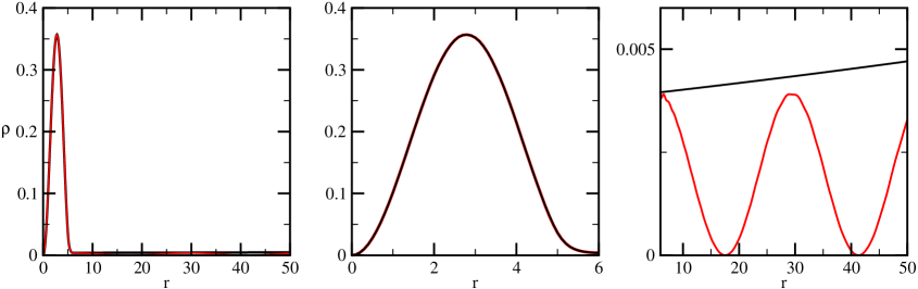
Figure 2: (color online) $\rho(r)$ for a $l=0$-resonant state, exact (black line) and Ritz-DO approximation with $N=100$ (red line) of the potential from Eq. (34). (a) global view. (b) Region $0\leq r\leq r_{0}=6$, where the resonant state is localized, and (c) The exterior region $r\geq r_{0}=6$, where the resonance diverges and the variational expansion is a stationary wave.

($ii$) The variational method gives good approximations to the exact (non-normalizable) densities $\rho(r)$ where the resonant states are localized (see figure 2).

($iii$) Eq. (22) involves just real quantities that could be evaluated with Ritz-variational wave functions.

Even Eqs. (22) and (25) are valid for $R\geq r_{0}$, because item ($ii$), in the numerical calculations we take $R=R_{0}=r_{0}$, and then $\int_{0}^{R_{0}}\;dr\left|u_{E,l}(r)\right|^{2}=1$.

III.1 $l=0$

We begin with the simple case of $s-$waves, $l=0$

For a clear notation, we will omit the subindexes $E$ and $l=0$, then $u(r)$ for an arbitrary potential $V(r)$ has the form

$$u(r)\,=\,\left\{\begin{array}[]{ll}u^{<}(r)&\mbox{if}\,r<r_{0}\\ u^{<}(r_{0})\,e^{ik(r-r_{0})}&\mbox{if}\,r>r_{0}\end{array}\right.\,.$$ (26)

Then, in this case Eq. (25) takes the form

$$\Gamma\,=\,\left[2\,{\cal E}\,+\,\left(\frac{\left|u^{<}(r_{0})\right|^{2}}{2}\right)^{2}\right]^{1/2}\,\left|u^{<}(r_{0})\right|^{2}\,.$$ (27)

Eq. (27) involves two real quantities, $\left|u^{<}(r_{0})\right|^{2}$ and ${\cal E}$, both quantities are well approximated by applying the Ritz method using a real square-integrable basis set truncated at order $N$, $\{\Phi_{i}\}_{1}^{N}$. In this approximation, the Hamiltonian $H_{l}$ is replaced by a $N\times N$ Hermitian matrix $[H_{l}]_{i,j}=\langle\Phi_{i}|H_{l}|\Phi_{j}\rangle$, and we obtain $N$ eigenvalues $E_{n}$ and eigenvectors $\vec{a}^{(n)}$. The corresponding orthonormal eigenfunctions are

$$\psi_{n}^{(N)}(r)\,=\,\sum_{i=1}^{N}\,a^{(n)}_{i}\,\Phi_{i}(r)\;\;\;;\;\;\;\sum_{i=1}^{N}\,\left(a^{(n)}_{i}\right)^{2}\,=\,1\;;\;n=1,\ldots,N\,.$$ (28)

In particular, we used the double-orthogonality method (DO) pots10 in order to calculate the real part of the resonant energy ${\cal E}^{(N)}$ and the variational square-integrable approximation to the resonant wave function $u^{(N)}(r)$. This method assumes that the potential depends on a parameter $\lambda$, and when $\lambda$ is varied on an interval $[\lambda_{L},\lambda_{R}]$ a given eigenvalue $n_{0}$ crosses the resonant energy value at $\lambda_{n_{0}}$, as illustrated in figure 1. The method uses the fact that in both sides of the interval, $\lambda_{L}$ and $\lambda_{R}$, the $n_{0}$ eigenvalues and eigenvectors in the left and in the right of the avoiding-crossing zone correspond to different states of the quasi-continuum and the resonant state is orthogonal to both of them. We define the double-orthogonality function

$$D_{n}(\lambda)=|\langle\psi_{n}(\lambda_{L}),\psi_{n}(\lambda)\rangle|^{2}+|\langle\psi_{n}(\lambda_{R}),\psi_{n}(\lambda)\rangle|^{2},\;\;\;\mbox{for}\;\lambda_{L}<\lambda<\lambda_{R}\,.$$ (29)

Because the eigenfunctions are normalized, $0\leq D_{n}(\lambda)\leq 2$. For a given eigenvalue $n_{0}$, we define the localization of the resonance $\lambda_{n_{0}}$ as the value of $\lambda$ where $D_{n_{0}}(\lambda)$ reaches its minimum, that is, where the eigenfunction has a minimum projection onto to the quasi-continuum states, at it is shown in figures 3 and 6. This method has the advantage over other stabilization methods in that we have to solve the variational problem just a single time. The price we pay is that $\lambda_{n}$ is also an output of the method and we cannot choose it arbitrarily. The best approximation of the resonance is defined as

$$\lambda_{n_{0}}\,=\,\min_{\lambda\epsilon[\lambda_{L},\lambda_{R}]}\,D_{n_{0}}(\lambda)\;\;\;;\;\;\;{\cal E}(\lambda_{n_{0}})\,=\,E_{n_{0}}(\lambda_{n_{0}})$$ (30)

Once we determine the optimal $\lambda_{n_{0}}$, its eigenfunction $\psi_{n_{0}}^{(N)}(r)$ pots10 together the normalization condition Eq. (15) give

$$u^{(N)}(r)\,=\,\frac{\psi_{n_{0}}^{(N)}(r)}{\int_{0}^{r_{0}}\,\left|\psi^{(N)}_{n_{0}}(r)\right|^{2}\,dr}\,=\,\frac{\sum_{i=1}^{N}\,a^{(N)}_{i}\,\Phi_{i}(r)}{\sqrt{\sum_{i,j=1}^{N}\,a^{(N)}_{i}a^{(N)}_{j}I_{i,j}(r_{0})}}\,,$$ (31)

where

$$I_{i,j}(R)\,=\,\int_{0}^{R}\,\Phi_{m}(r)\,\Phi_{n}(r)\,dr\,.$$ (32)

Then, from Eq. (27) we obtain for $\Gamma^{(N)}$

$$\Gamma^{(N)}\,=\,\frac{\left(\psi_{n_{0}}^{(N)}(r_{0})\right)^{2}}{\sum_{i,j=1}^{N}\,a^{(N)}_{i}a^{(N)}_{j}I_{i,j}(r_{0})}\;\left[\left(\frac{\left(\psi_{n_{0}}^{(N)}(r_{0})\right)^{2}}{2\,\sum_{i,j=1}^{N}\,a^{(N)}_{i}a^{(N)}_{j}I_{i,j}(r_{0})}\right)^{2}\,+\,2\,{\cal E}\right]^{1/2}\;.$$ (33)

As a particular case, we calculated resonant states for an exactly solved problem, the well+barrier potential hogreve95

$${\cal V}(r)\,=\,\left\{\begin{array}[]{ll}-V_{0}&\mbox{if}\,r<\Delta\\ +\lambda&\mbox{if}\,\Delta<r<r_{0}\end{array}\right.\,,$$ (34)

where all the parameters are positive. The exact wave functions are different combinations of exponential functions in each sector, with continuous logarithm derivative at $r=\Delta$ and $r=r_{0}$. The exact energies for bound, virtual and resonant states are given as solutions of three different transcendental algebraic equations, which are obtained applying the corresponding boundary condition at $r=r_{0}$ hogreve95 .

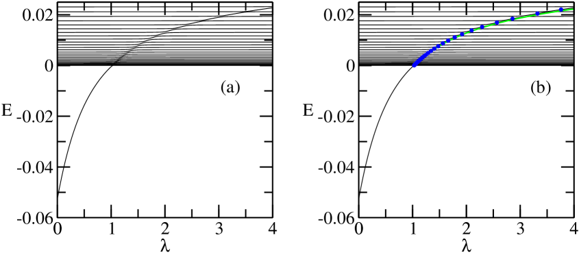
Figure 1: (color online) (a) The first 30 eigenvalues of the $N=100$ Hamiltonian matrix of the $l=0$ block of the potential Eq. (34) as a function of the barrier height $\lambda$. (b) Same as (a) plus exact (green line) and approximate (blue dots) energies of the resonant state.

Figure 3: $D_{n}$ for the $l=0$ block of the potential Eq. (34) as a function of the barrier height $\lambda$ for $N=100$ and $n=2,\ldots,30$. The minimum of each curve is defined as the localization of the resonant state.

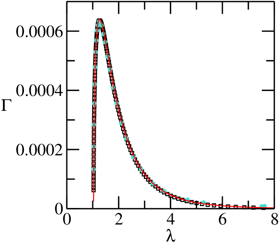
Figure 4: (color online) Exact (red line), $N=100$ (turquoise dots) and $N=500$ (black squares) values of $\Gamma$ against the barrier height $\lambda$ for the $l=0$ block of the potential Eq. (34).

The calculations were done as a function of the barrier height $\lambda$, with fixed values of $V_{0}=0.15,\,\Delta=5$, and $r_{0}=6$. A convenient orthonormal basis set is given by

$$\Phi_{i}(r)\,=\,\frac{1}{\sqrt{(i+1)(i+2)}}\,e^{-r/2}L^{(2)}_{i}(r)\;;\;i=1,\ldots,N\,.$$ (35)

where $L^{(2)}_{i}(r)$ is the Laguerre polynomial of degree $i$ and order 2 abramowitz .

In figure 1(a) we show the first thirty eigenvalues given by the Ritz method with $N=100$. In figure 1(b) we add the exact resonant energy curve and the values calculated with the $DO_{n}$ functions, which are shown in figure 3 for $N=100$, and $n=2,\ldots,30$. Once the energy was obtained, the width $\Gamma$ of the resonance is calculated using Eq. (33). In figure 4 we show $\Gamma(\lambda_{n})$ for two different sizes of the basis set: $N=100$, for $n=2,\ldots,30$, and $N=500$, for $n=2,\ldots,140$. Our data show an excellent agreement with the exact curve $\Gamma(\lambda)$, that is also included in the figure.

III.2 $l=1$

From Eq. (24), the function $v_{l}(k,r)$ for $p$-waves takes the form

$$v_{1}(k,r_{0})\,=\,1+\frac{i}{kr_{0}}\,.$$ (36)

In this case, it is convenient to re-write Eq. (22) as a function of $x\equiv Im(k)$

$$x^{3}\,+\,\left(\frac{1}{r_{0}}\,+\,\frac{\left|u(r_{0})\right|^{2}}{2}\right)\,x^{2}\,+\,\left({\cal E}\,+\,\frac{1}{2r_{0}^{2}}\,+\,\frac{\left|u(r_{0})\right|^{2}}{2r_{0}}\right)\,x\,+\,{\cal E}\,\frac{\left|u(r_{0})\right|^{2}}{2}\,=\,0\,.$$ (37)

The definition of resonance establish that $Im(k)>0$, and we proved for each case that we studied that Eq. (37) has an unique positive root. Finally $\Gamma$ is obtained from the definition of $k$ as

$$\Gamma\,=\,-2\,x_{p}\,\sqrt{2\,{\cal E}\,+\,x_{p}^{2}}\,,$$ (38)

where $x_{p}$ is the positive root of Eq. (37).

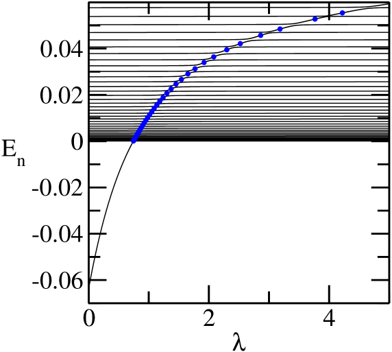
Figure 5: (color online) The first 30 eigenvalues of the $N=100$ Hamiltonian matrix of the $l=1$ block of the potential Eq. (34) as a function of the barrier height $\lambda$. The approximate energies of the resonant state calculated with DO are also shown (blue dots).

Figure 6: $D_{n}$ for the $l=1$ block of the potential Eq. (34) as a function of the barrier height $\lambda$ for $N=100$ and $n=2,\ldots,30$. The minimum of each curve is defined as the localization of the resonant state.

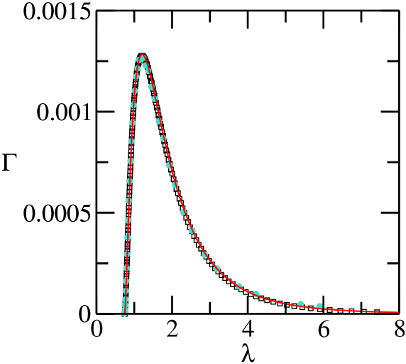
Figure 7: (color online) Exact (red line), $N=100$ (turquoise dots) and $N=500$ (black squares) values of $\Gamma$ against the barrier height $\lambda$ for the $l=1$ block of the potential Eq. (34).

We calculated the inverse lifetime $\Gamma$ for a $l=1$ resonant state of the potential Eq. (34) as a function of the barrier height $\lambda$, with fixed values of $V_{0}=0.3,\,\Delta=5$, and $r_{0}=6$. In figure 5 we show the first thirty eigenvalues of the $N=100$ $p$-block of the Hamiltonian matrix and the resonant energies ${\cal E}$ calculated with the DO method. The curves $D_{n}(\lambda)$ for $n=2,\ldots,30$ are shown in figure 6. Note the qualitative differences between the DO curves for $l=0$ and $l=1$ in figures 3 and 6 respectively. These differences are due to the existence of a virtual state between the bound and the resonant states for the $l=0$ case, which it is absent in the $l=1$ case, where the bound state is continued directly in a resonant state.

In figure 7 we show the exact curve $\Gamma$ vs. $\lambda$ and the approximate values obtained with two different basis-set size: $N=100$, for $n=2,\ldots,40$ and $N=500$, for $n=2,\ldots,200$. As in the case with zero angular momentum, we obtain an excellent agreement between exact and approximate results.

IV conclusions

In this work we used a probabilistic interpretation of resonant (Siegert) states based on the conservation of the number of particles inside a time-dependent volume hatano08 ; hatano09 ; hatano10 . The advantage of the probabilistic interpretation of resonant states is that is possible to work with Siegert states in a similar way to bound states, calculating probabilities, expectation values, etc.

In particular, we obtain the exact equation (22), which reduces to Eq. (25) and Eq. (37) for $l=0$ and $l=1$ respectively. These equations relate the inverse lifetime with other real magnitudes, the energy and the density of a resonance. In previous papers, once the energy of a resonance is obtained applying a real algebra stabilization-like method, the resonance width is calculated performing a fitting of the density of states (kh04 and references therein, pots10 ). In the present work Eq. (22) gives a value for $\Gamma$ with the same degree of accuracy that we obtain for the energy of the resonance ${\cal E}$.

We emphasize the simplicity of the calculations compared to other methods that use complex algebra to study resonant states. We present our results for potentials with finite support, but Eq. (22) is valid in general, and the calculation of $\Gamma$ could be corrected by a systematic perturbative expansion.

An open question is if Eq. (22) could be generalized for few-particle systems, where many channels are present. We are working in this direction.

- (1) G. Gamow, Z. Phys. 51, 204 (1928).
- (2) E. Brändas and N. Elandar (eds), Resonances (Springer-Verlag, Berlin, Heidelberg, 1989).
- (3) T. Sommerfeld and L.S. Cederbaum, Phys. Rev. lett. 80, 3723 (1998).
- (4) N. Moiseyev and C. Corcoran, Phys. Rev. A 20, 814 (1979).
- (5) M Bylicki, W Jaskólski, A Stachów and J Diaz, Phys. Rev. B 72, 075434 (2005).
- (6) A. D. Dente, R. A. Bustos-Marún and H. M. Pastawski, Phys. Rev. A 78, 062116 (2008).
- (7) A. Ferrón, O. Osenda and P. Serra, Phys. Rev. A 79, 032509 (2009).
- (8) N. Hatano, K. Sasada, H. Nakamura and T. Petrosky, Prog. Theor. Phys. 119, 187 (2008).
- (9) N Hatano, T. Kawamoto and J. Feinberg, Pramana J. Phys. 73, 553 (2009).
- (10) N Hatano, Prog. Theor. Phys. Supp. 184, 497 (2010).
- (11) A. J. F. Siegert, Phys. Rev. 56, 750 (1939).
- (12) N. Moiseyev, Phys. Rep. 302, 211 (1998).
- (13) N Moiseyev, Non-Hermitean Quantum Mechanics, Cambridge University Press (2011).
- (14) C. W. McCurdy, M. Baertschy, and T. N. Rescigno, J. Phys. B 37, R137 (2004).
- (15) A. Palacios, T. N. Rescigno, and C. W. McCurdy, Phys. Rev. A 79, 033402 (2009).
- (16) L. Tao, C. W. McCurdy, and T. N. Rescigno, Phys. Rev. A 82, 023423 (2010).
- (17) V. A. Mandelshtam, T. R. Ravuri, and H. S. Taylor, Phys. Rev. Lett. 70, 1932 (1993).
- (18) A.U. Hazi and H. S. Taylor, Phys. Rev. A 1, 1109 (1970).
- (19) S. Kar and Y. K. Ho, J. Phys. B: At. Mol. Opt. Phys. 37 3177 (2004).
- (20) F. M. Pont, O. Osenda, J.H. Toloza and P. Serra, Phys. Rev. A 81, 042518 (2010).
- (21) F. M. Pont, O. Osenda and P. Serra, Phys. Scrip. 82, 038104 (2010).
- (22) See any textbook on quantum mechanics, for example E. Merzbacher, Quantum Mechanics, third edition, John Wiley, New York (1998).
- (23) H. Hogreve, Phys. Lett. A 201, 11 (1995).
- (24) M. Abramowitz, and I. Stegun (eds.), Handbook of mathematical functions, Dover Publications, 9 ed. New York, 1972.