Criticality in Alternating Layered Ising Models :
I. Effects of connectivity and proximity

Abstract

The specific heats of exactly solvable alternating layered planar Ising models with strips of width $m_{1}$ lattice spacings and “strong” couplings $J_{1}$ sandwiched between strips of width $m_{2}$ and “weak” coupling $J_{2}$, have been studied numerically to investigate the effects of connectivity and proximity. We find that the enhancements of the specific heats of the strong layers and of the overall or ‘bulk’ critical temperature, $T_{c}(J_{1},J_{2};m_{1},m_{2})$, arising from the collective effects reflect the observations of Gasparini and coworkers in experiments on confined superfluid helium. Explicitly, we demonstrate that finite-size scaling holds in the vicinity of the upper limiting critical point $T_{1c}$ ($\propto J_{1}/k_{B}$) and close to the corresponding lower critical limit $T_{2c}$ ($\propto J_{2}/k_{B}$) when $m_{1}$ and $m_{2}$ increase. However, the residual enhancement, defined via appropriate subtractions of leading contributions from the total specific heat, is dominated (away from $T_{1c}$ and $T_{2c}$) by a decay factor $1/(m_{1}+m_{2})$ arising from the seams (or boundaries) separating the strips; close to $T_{1c}$ and $T_{2c}$ the decay is slower by a factor $\ln m_{1}$ and $\ln m_{2}$, respectively.

I Introduction

Many experiments performed on ⁴He at the superfluid transition in various spatial dimensions,GKMD reveal excellent agreement with general finite-size scaling theory.Fisher ; Barber Furthermore, when small boxes or “quantum dots” of helium were coupled through a thin helium film, effects of connectivity and proximity were discovered and quantified.PKMG ; KMG ; PKMGn ; MEF ; PG ; PKMGpr

To gain some more detailed theoretical insights into the proximity effects, we study here the specific heats of an alternating layered planar Ising model, which consists of infinite strips of width $m_{1}$ lattice spacings in which the coupling or bond energy between the nearest-neighbor Ising spins is $J_{1}$, separated by other infinite strips of width $m_{2}$ bonds (or lattice spacings) whose coupling $J_{2}$ is weaker. This is illustrated in Fig. 1.

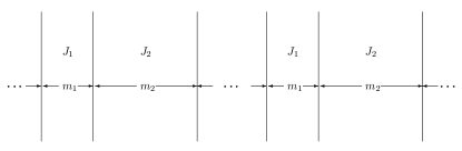
Figure 1: The planar, square lattice alternating layered Ising model considered. The widths $m_{1}$ and $m_{2}$ are measured in nearest-neighbor lattice spacings, $a$, while nearest-neighbor Ising spins $\sigma_{i}=\pm 1$ are coupled via pair Hamiltonians $J_{ij}\sigma_{i}\sigma_{j}$ with $J_{i,j}=J_{1}$ or $J_{2}$ as illustrated schematically. On the seams at lattice sites with $x=n(m_{1}+m_{2})a+a$ for $n=0,\pm 1,\pm 2,\dots$, the vertical bonds are of energy $J_{1}$ while the horizontal bonds are of strength $J_{1}$ on the right but $J_{2}$ on the left; conversely, for the seams at $x=(n+1)m_{1}a+nm_{2}a+a$ the vertical bonds have strength $J_{2}$ while the horizontal bonds on the right are of energy $J_{2}$ but $J_{1}$ on the left.

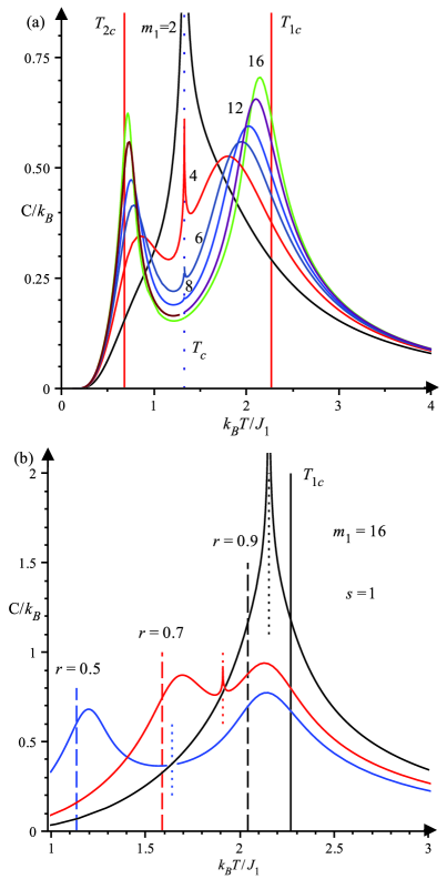
Figure 2: (Color online) (a) The specific heats per site with relative strength $r=J_{2}/J_{1}=0.3$ and relative separation $s=m_{2}/m_{1}=1$ for $m_{1}=2,4,\cdots,16$. The amplitude $A(r,s)$ of the logarithmic divergence at $T_{c}(r,s)$, which dominates for $m_{1}=2$, decreases rapidly as $m_{1}$ increases. Thus, the small spike at the “true” bulk critical point, $T_{c}$ (indicated by the dotted vertical line), becomes barely visible for $m_{1}\geq 8$. (b) Plots of the specific heats for fixed $m_{1}=m_{2}=16$ and so $s=1$ but for increasing relative strength $r$. Note that the logarithmic peak at the overall or bulk critical point, $T_{c}(r,s)$, indicated by short vertical dotted lines, remains clearly visible when $r=0.7$ and still dominates entirely when $r=0.9$. The vertical dashed lines denote the positions of $T_{2c}(r)$. Unlike part (a), now the spike remains evident at $m_{1}=16$ when $r\uparrow 1$. However, as $A(r,s)$ becomes small, two quite distinct rounded peaks appear moving toward the limiting values $T_{2c}(r)$ (denoted by vertical dashed lines) and $T_{1c}$, as $m_{1}=m_{2}\to\infty$.

When $J_{2}$ vanishes, the model becomes a system of noninteracting infinite strips of finite width, each of which essentially behaves as a one-dimensional Ising model. This means, in particular, that the specific heat is not divergent but rather has a fully analytic rounded peak. However, as long as $J_{2}\neq 0$, the system is a two-dimensional bulk Ising model, whose specific heat per site diverges logarithmically at a unique bulk critical temperature $T_{c}(J_{1},J_{2};m_{1},m_{2})$ in the form

$$C(T)/k_{B}\propto-A(r,s)\ln|1-(T/T_{c})|+B(r,s)+\cdots,$$ (1)

where we have introduced the basic weakness or coupling ratio, $r$, and the relative separation distance, $s$, namely

$$\quad r=J_{2}/J_{1}<1,\quad s=m_{2}/m_{1}.$$ (2)

In fact, as will be shown in Part II,HAY the amplitude $A(r,s)$ of the logarithmic divergence decays exponentially as a function of $m_{1}$ or of $m_{2}$;HAY indeed, at fixed $s$ and $r\to 1$, the amplitude decays as $Pm_{1}{\rm e}^{-Pm_{1}}$, where $P\propto(1-r)s/(1+s)$ as $m_{1}\to\infty$. This behavior is evident for $r=0.3$ in Fig. 2(a), which shows that the divergence, while obvious and dominant for $m_{1}=m_{2}<3$, rapidly becomes no more than a minuscule spike, which soon becomes invisible on any graphical plot. On the other hand, for greater values of the coupling ratio $r$ the logarithmic divergence remains dominant for larger values of $m_{1}$ and $m_{2}$ as seen in Fig. 2(b). But returning to Fig. 2(a) with $r=0.3$, one observes that as soon as the strip widths, $m_{1}=m_{2}$, exceed three lattice spacings, there appear two further specific heat peaks, albeit rounded; these grow rapidly in height and sharpness, and as $m_{1}$ and $m_{2}$ increase, they soon dominate the plots.

Now Fig. 2 is based on exact analytic calculations expounded in Part II of this article.HAY In fact, the analysis of the finite-size behavior of planar Ising models based on the exact solution of Onsager, as extended by Kaufman,Kaufman goes back to the work of Fisher and FerdinandFerdFisher ; MEFJp in 1969. Specifically, the solubility of arbitrarily layered planar Ising models was first noted and reported at a conference in Japan,MEFJp while, independently, McCoy and WuMWbk developed and analyzed randomly layered Ising models. The thermodynamics for regularly layered models was developed by Au-Yang and McCoyHAYBM and Hamm,Hamm while the scaling behavior of a single strip of finite width was elucidated by Au-Yang and Fisher.HAYFisher

In general the bulk critical temperature can be simply stated, for a layered distribution as MEFJp

$$k_{B}T_{c}\langle\!\langle\ln\coth(J_{x}/k_{B}T_{c})\rangle\!\rangle=2\langle\!\langle J_{y}\rangle\!\rangle,$$ (3)

where the brackets $\langle\!\langle\cdot\rangle\!\rangle$ denote an average over the distribution, random or regular of the distinct number (say $n<\infty$) of lattice spacings constituting a layer of finite width. For the alternating layered Ising model, this becomes

$$2J_{1}(1+rs)$$

$$=k_{B}T_{c}[\ln\coth(J_{1}/k_{B}T_{c})+s\ln\coth(rJ_{1}/k_{B}T_{c})],$$ (4)

which depends only on the weakness ratio $r$ and the relative separation $s$.

Then as $m_{1}$ and $m_{2}$ become large, the upper and lower rounded peaks approach limiting values, $T_{1c}$ and $T_{2c}$ (as evident in Fig. 2(a)), which, in fact, match the corresponding bulk (i.e., uniform) two-dimensional Ising models with coupling constants $J_{1}$ and $J_{2}$. Thus the limiting values $T_{1c}$ and $T_{2c}(r)$ are known Kaufman ; FerdFisher ; MWbk and given by

$$k_{B}T_{1c}/J_{1}\simeq 2.269185312,$$

$$k_{B}T_{2c}/J_{1}\simeq r\cdot 2.269185312.$$ (5)

It proves easy to establish the expected inequalities

$$T_{2c}(r)\leq T_{c}(r,s)\leq T_{1c}.$$ (6)

II Qualitative Observations

Figure 3: (Color online) The specific heats of alternating layered Ising models with relative strength $r=\!0.3$ (as in Fig. 2 (a)) and relative separation $s=2$ for $m_{1}=8,16$. The dashed plots denote the corresponding decoupled specific heats when $J_{2}=0$ ($r=0$), while the dotted lines represent the specific heats when $J_{1}=0$ (or $r\to\infty$). The inset displays the distinct maxima near $T_{2c}$, dotted below but solid above.

To explore further and develop the analogies with the observations on superfluid helium systems, we retain the value of the weakness ratio $r=0.3$ (used in Fig. 2(a)) but increase the relative layer separation to $s=2$. The results for $m_{1}=8$ and 16 (as used in Fig. 2(a)) are presented in Fig. 3: see the solid curves. As anticipated, no sign of any singularity at $T_{c}$ is visible. It should be noted, nonetheless, that were one to examine the overall spontaneous magnetization, $M_{0}(T)$, one would find — and on a plot see — that $M_{0}$ vanished identically for $T>T_{c}$ but was nonzero (and varying as $\propto(T_{c}-T)^{\beta}$ with $\beta={\textstyle\frac{1}{8}}$ for 2D Ising layersFisher ; Barber ; MWbk ) as soon as $T<T_{c}$. In the experiments on superfluids the analogous statement concerns the overall superfluid density $\rho_{s}(T)$;GKMD this vanishes identically above the overall or bulk lambda transition at $T_{\lambda}(\equiv T_{c})$ but is detectable, via setting up persistent superflow fluid currents, below $T_{\lambda}$.PKMGn ; PG (In a bulk 3D superfluid $\rho_{s}(T)$ varies as $(T_{\lambda}-T)^{\zeta}$ with $\zeta\simeq 0.67$, but in a planar 2D superfluid film of thickness $L$, $\rho_{s}(T)$ increases discontinuously at the corresponding superfluid transition temperature, $T_{c}(L)$, on lowering the temperature.GKMD )

On the other hand, the temperatures of the upper and lower rounded maxima increase (and decrease, respectively), as $m_{1}$ increases in Fig. 3. But now, using the explicit results for the infinite strip of finite width,HAYFisher we also show, as dashed curves in Fig. 3, the totally decoupled $r=0$ (or $J_{2}=0$) plots for the two cases $m_{1}=8$ and $16$. Clearly the uncoupled upper maxima fall below $T_{1c}$ just as do the coupled ($r=0.3$) results. (It is worth remarking, however, that for a finite $n\times n$ Ising lattice with periodic boundary conditions, as studied by Ferdinand and Fisher,FerdFisher the maxima in the specific heats lie above the bulk critical temperature $T_{1c}$.) Nevertheless, there is clear evidence of a coupling or proximity effect in that the specific heats for the alternating, coupled system lie markedly above those for the decoupled ($r=0$) strips. This same effect is seen in the experiments when finite boxes are coupled by a helium film.PKMGn ; PG

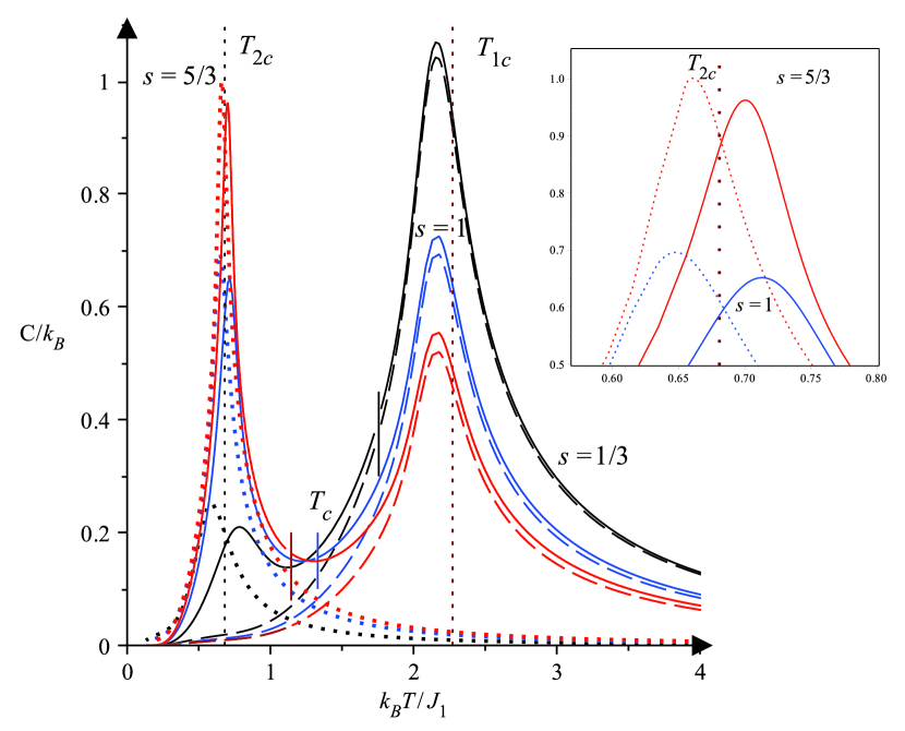
Figure 4: (Color online) Specific heat plots for relative strength $r=0.3$ (as in Figs. 2(a) and 3) but with relative separations $s=1/3,1$ and $5/3$ when $m_{1}=18$. Again the decoupled $r=0$ behavior is seen in the dashed plots while for the opposite limit, $r\to\infty$, the plots are dotted. The short vertical lines locate the bulk critical points, $T_{c}(r,s)$, which decrease as $s$ increases. The inset shows various coupled and uncoupled maxima near $T_{2c}$.

Complementary phenomena are observed around the lower maxima. Thus the dotted plots in Fig. 3 show the finite-width result for the situation $r\to\infty$, or, more intuitively, $J_{1}=0$, for $m_{1}=8$ and $16$ (i.e., $m_{2}=16$ and $32$). These decoupled specific heats appear as very sharp, but still finitely rounded, spikes. However, it must be noted that these $r\to\infty$ maxima lie below $T_{2c}$, in accord with expectation for a finite-width strip. On the other hand, the maxima of the coupled alternating system lie above the limiting value $T_{2c}$ as seen clearly in the inset in Fig. 3. Once again there is an unmistakable proximity or enhancement effect that is found also in the experimental studies.PKMGn ; PG

As a next step of our qualitative exploration, we present in Fig. 4 the effects of varying the relative separation $s$ for significantly wide, $m_{1}=18$, strips spaced apart by weaker strips of relative strength $r=0.3$ (as before). In this case the first point to notice is that $T_{c}(r,s)$ increases quite rapidly towards $T_{1c}$ as the separation $s$ approaches zero. Next, the uncoupled ($r=0$) specific heats near $T_{1c}$ (shown dashed as in Fig. 3) all have maxima located at the same temperature, determined only by $m_{1}=18$ for a finite width strips, while their magnitude is determined by $s$ simply via normalization, either through relative area or on a per-site basis. However, there is still clear enhancement in the coupled layers even though the corresponding rounded maxima deviate very little in location from the uncoupled case. By contrast near $T_{2c}$, as illustrated by the inset, the displacements even of the uncoupled maxima (shown dotted), depend significantly on the relative separation ratio $s$. Again, nonetheless, there is proximity induced enhancement of the peaks both in magnitude and displacement above $T_{2c}$.

Finally, we may enquire about the level of the specific heats around the bulk critical point $T_{c}$ or in the vicinity of the minima observed in Figs. 2-4 that lie roughly at $T_{min}\lesssim{\scriptstyle\frac{1}{2}}(T_{1c}+T_{2c})$. One may ask, for example, how well the levels are approximated by appropriately weighted sums of the uncoupled peaks around $T_{1c}$ plus some, perhaps reversed contribution from $T_{2c}$. For these purposes, however, we need to proceed more quantitatively.

III Scaling Explorations Near The Maxima

We would like to relate the observations embodied in Figs. 2-4 to more general scaling concepts. To this end, recallFisher ; Barber ; MEFJp ; FerdFisher that a bulk system with a critical temperature $T_{c}$ may be characterized by a correlation length $\xi(T)$ which diverges on approach to criticality as

$$\xi(T)\approx\xi_{0}/|t|^{\nu}\quad\hbox{with}\quad t=(T/T_{c})-1\to 0,$$ (7)

where $\nu$ is a characteristic critical exponent while $\xi_{0}$ is a length of order the lattice spacing $a$, or molecular size, etc. For 2D Ising systems one hasFisher ; Barber ; FerdFisher ; MWbk $\nu=1$, whereas for superfluid helium in three bulk dimensions $\nu\simeq 0.67$.GKMD Then in a system limited in size by a finite length $L=\ell a$, the scaling hypothesis asserts, in general terms, that when $\ell$ and $\xi(T)$ are large enough, the rounding of critical point singularities is primarily controlled by the ratio $y=L/\xi(T)$.

Consequently, for the finite-size behavior of the specific heat per site, which diverges in bulk as $|t|^{-\alpha}$ where $\alpha$ is typically small (or even negative), the basic scaling hypothesis may be expressed as

$$C(\ell;T)\approx\ell^{\alpha/\nu}[Q(x)-Q_{0}]/\alpha,$$ (8)

where $Q(x)$ is the scaling function while the scaled temperature is

$$x=\ell^{1/\nu}t\propto y^{1/\nu}=[L/\xi(T)]^{1/\nu},$$ (9)

and $Q_{0}>0$ is a constant parameter. The exponent $\alpha$ in the denominator in (8) allows for the limit $\alpha\to 0$, which yields, with $Q(0)\to Q_{0}$, a logarithmic singularity as is appropriate for 2D Ising systems. One may then take

$$C(\ell;T)\approx(Q_{0}/\nu)\ln\ell+Q(\ell^{1/\nu}t)$$ (10)

as the basic hypothesis where, for use below, we note that at criticality one has $C(\ell;T_{c})\approx(Q_{0}/\nu)\ln\ell+Q(0)$. In fact, this hypothesis has been established explicitly for infinite Ising strips of width $\ell$ and $Q(x)$ has been explicitly determined.HAYFisher

III.1 Upper Maxima near ${\bf T_{1c}}$

To apply these concepts to our layered Ising system, in the first case for the upper maxima near $T_{1c}$, we recall from Figs. 3 and 4 that leaving aside relatively small enhancements in magnitude, the total specific heat, $C(J_{1},J_{2};T)$, approaches rather well the limiting formsHAYFisher of a suitably normalized single strip of width $m_{1}$. Accordingly, we subtract a contribution from non-coupled weaker Ising strips by defining

$${C_{1}}(J_{1},J_{2};T)=(1+s)[C(J_{1},J_{2};T)-C(0,J_{2};T)],$$ (11)

where the normalization factor $(1+s)$ is needed for the scaling plots now to be examined. Finally in accord with (10) and the subsequent remark we introduce the upper or stronger net finite-size contribution

$$\Delta{C_{1}}(J_{1},J_{2};T)=C_{1}(J_{1},J_{2};T)-C_{1}(J_{1},J_{2};T_{1c}),$$ (12)

in which the value at the limiting critical point, $T_{1c}$, has been subtracted. If we accept the identifications $\ell\Rightarrow m_{1}$ and $t\Rightarrow t_{1}=(T/T_{1c})-1$ and recall $\nu=1$, we might expect $\Delta C_{1}(T)$ to obey scaling in terms of the scaled temperature variable

$$x_{1}=m_{1}[(T/T_{1c})-1]\equiv m_{1}t_{1}.$$ (13)

This expectation is well supported by the plots in Fig. 5 for $m_{1}=18$ and $s=n/3$ for $n=1,2,\cdots,5$: the “data collapse” is strikingly well realized.

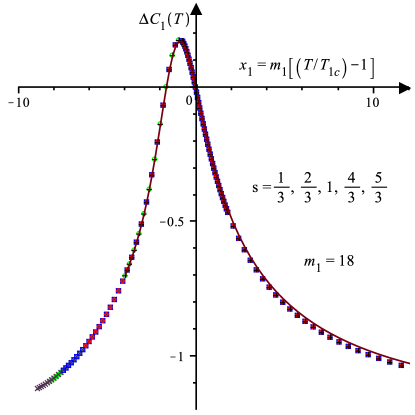
Figure 5: (Color online) Scaling plot vs $x_{1}=m_{1}t_{1}$ for the upper or stronger net finite-size contribution, namely, $\Delta{C}_{1}(J_{1},J_{2};T)$ as defined in the text for strong strips of width $m_{1}=18$ at various separations but fixed $r=0.3$. The solid curve is the plot of the specific heat of an infinite strip of width $m_{1}=18$ and coupling $J_{1}$ when its value at the bulk critical temperature $T_{1c}$ is subtracted.HAYFisher

Beyond this, however, explicit calculations HAY show that, asymptotically, $\Delta C_{1}(T)$ is simply related to the limiting scaling function, $Q^{\infty}(x_{1})$, for an infinite strip of coupling $J_{1}$ and width $m_{1}$ already known explicitly.HAYFisher Specifically, allowing for normalization, yields

$$\Delta{C_{1}}(J_{1},J_{2};T)\approx(1+s)[C(J_{1},0;T)-C(J_{1},0;T_{1c})]$$

$$\qquad\approx Q^{\infty}(x_{1})-Q^{\infty}(0),$$ (14)

where, to complete the description we reportHAY

$$(1+s)C_{1}(J_{1},J_{2};m_{1},m_{2};T_{1c})\approx C^{\infty}(J_{1};m_{1};T_{1c})$$

$$\qquad\approx A_{0}\ln m_{1}+Q^{\infty}(0);$$

$$A_{0}=2[\ln(\sqrt{2}+1)]^{2}/{\pi},\quad Q^{\infty}(0)\approx 0.30681A_{0},$$ (15)

which (recognizing that $\nu=1$ for 2D Ising models) is in accord with (10). Note that in this limit not only has the dependence on $m_{2}$ dropped out but also the dependence on $J_{2}$. However, as regards the enhancement seen in Figs. 2-4, we know that $m_{2}$ and $J_{2}$ do play a role. This will be studied further below.

III.2 Lower Maxima near ${\bf T_{2c}}$

Let us now shift attention to the behavior of the specific heat peaks of the alternating system, near the lower (or weaker) limiting critical point, $T_{2c}$. The rounded maxima are shown in detail in the insets of Figs. 3 and 4. Now we can follow the procedure that led to the definition (11). Thus we consider the normalized difference

$${C_{2}}(J_{1},J_{2};T)=(1+s^{-1})[C(J_{1},J_{2};T)-C(J_{1},0;T)].$$ (16)

Then, following again the previous analysis, the weaker net finite-size contribution may be defined as in (12), by

$$\Delta{C_{2}}(J_{1},J_{2};T)=C_{2}(J_{1},J_{2};T)-C_{2}(J_{1},J_{2};T_{2c}).$$ (17)

It is natural to suppose that $\Delta C_{2}(T)$ might obey scaling in terms of the new scaled temperature variable

$$x_{2}=m_{2}[(T/T_{2c})-1]\equiv m_{2}t_{2}.$$ (18)

Figure 6: (Color online) Scaling plots versus the scaling variable $x_{2}=m_{2}t_{2}$ for the lower or weaker net finite-size contribution $\Delta{C}_{2}(J_{1},J_{2};T)$, as defined in relations (16)-(17), for strips of width $m_{2}=16$ and $r=0.3$ for various relative separations. The solid curve represents the corresponding asymptotic form $Q^{\infty}(-x_{2})-Q^{\infty}(0)$, for an infinite strip of finite width and coupling $J_{2}$, with the temperature reflected about $T=T_{2c}$.HAYFisher The dashed curve represents data for a wider strip with $m_{2}=60$.

This hypothesis is tested in Fig. 6 and, evidently, is remarkably successful, exhibiting excellent data collapse. But more remarkable yet is the evidence provided by the solid line plotted in Fig. 6. This derives directly from the limiting scaling function for an infinite stripHAYFisher of coupling $J$ and finite width $m$ but with the sign of the argument reversed. In other words, the previous asymptotic form (14) is now, as established in Part II,HAY replaced by

$$\Delta{C_{2}}(J_{1},J_{2};T)\approx(1+s^{-1})[C_{2}(0,J_{2};{{\check{T^{\vphantom{{}^{\prime}}}}}})-C_{2}(0,J_{2};T_{2c})]$$

$$\qquad\approx Q^{\infty}(-x_{2})-Q^{\infty}(0),$$ (19)

where the modified temperature ${{\check{T^{\vphantom{{}^{\prime}}}}}}$ is simply attained by reflecting about $T_{2c}$; explicitly we have

$${{\check{T^{\vphantom{{}^{\prime}}}}}}(T)=T_{2c}-(T-T_{2c})=2T_{2c}-T.$$ (20)

It is appropriate to recall (15) which may now be rewritten to complement (19) as

$$(1+s^{-1})C_{2}(J_{1},J_{2};m_{1},m_{2};T_{2c})\approx C^{\infty}(J_{2};m_{2};T_{2c})$$

$$\qquad\approx A_{0}\ln m_{2}+Q^{\infty}(0),$$ (21)

in which the values of $A_{0}$ and $Q^{\infty}(0)$ are given in (15). We may note, further, that in this limit the original dependence on both $J_{1}$ and $m_{1}$ has vanished; but, once more, there are clear residual effects associated with the proximity and interlayer couplings.

IV Enhancement Effects

To address the behavior of the specific heats beyond the leading scaling behavior revealed in Figs. 5 and 6, we may define an “enhancement” by subtracting from the total specific heat per site contributions deriving from the corresponding independent uncoupled strips. However, in doing this we must recognize — following Fig. 6 and the result (19) — that a reversed or reflected temperature variable is needed around $T_{2c}$. To this end we utilize the modified temperature variable, ${{\check{T^{\vphantom{{}^{\prime}}}}}}(T)$, defined in (20). Thus we specify the net enhancement for fixed $m_{1}$ and $m_{2}$ by

$${\cal E}(J_{1},J_{2};m_{1},m_{2};T)$$

$$\quad=C(J_{1},J_{2};T)-C(J_{1},0;T)-C{\mbox{\boldmath$($}}0,J_{2};{{\check{T^{\vphantom{{}^{\prime}}}}}}(r){\mbox{\boldmath$)$}}.$$ (22)

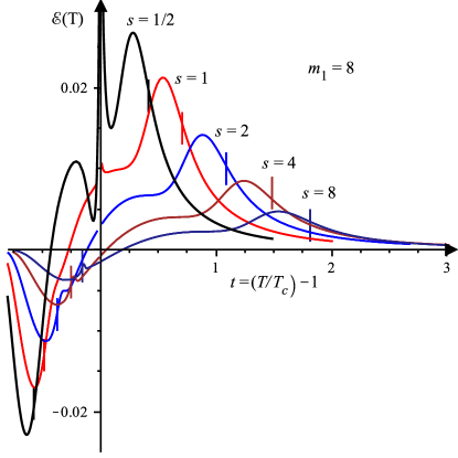
Figure 7: (Color online) Plots of the enhancement ${\cal E}(t)$ versus $t=(T/T_{c})-1$ for $m_{1}=8$, $r=0.3$ and various relative separations $s$. The short vertical lines above $T_{c}(r,s)$, i.e., for $t>0$, are the corresponding positions of $T_{1c}$, while below $T_{c}(r,s)$, they locate $T_{2c}$.

It is worth remarking parenthetically that in adopting this definition of the enhancement we are, in particular, utilizing the theoretical result (19) proved for the alternating Ising strips.HAY In more general situations (such as confined superfluid helium) the last term in (22) should be replaced by an asymptotic term obtained through an appropriate initial data analysis of the behavior close to $T_{2c}$ such as led to the original (finite $m_{2}$) form in Fig. 6.

In Fig. 7, we plot the enhancement for our alternating Ising strips with $r=0.3$ as a function of $t=[(T/T_{c})-1]$ for $m_{1}=8$ and various separations $s$. One sees that the logarithmic divergence at $t=0$ is barely visible for $s=1$, and essentially disappears for $s>1$. In addition, as expected, the magnitude of the enhancement decreases as $s$ (or $m_{2}$) increases; but by what law?

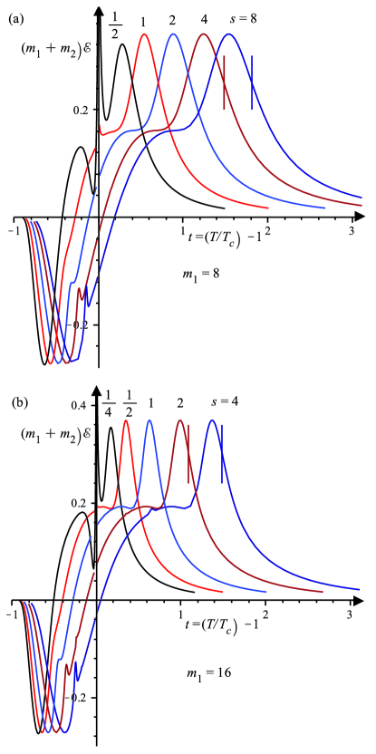
Figure 8: (Color online) The enhancement ${\cal E}(t)$ multiplied by $(m_{1}+m_{2})$: (a) for $m_{1}=8$ as in Fig. 7, and (b) for $m_{1}=16$. The short vertical lines locate the corresponding upper limiting critical points, $T_{1c}$.

To address this question we recall, first, that the leading correction to the asymptotic form of the specific heat of an infinite strip of finite width $m$ must arise from the two non-vanishing boundary free energy contributionsFerdFisher ; MWbk ; HAYFisher ; FisherFerd which yield a total specific heat term of relative order $1/m$. The effects of this are already evident in Fig. 6 where the primary contribution (solid curve) is, especially for $x_{2}\geq 2$, more closely approached by the data for $m_{2}=60$ than that for $m_{2}=16$. It is clear that such corrections must arise also in the bulk alternating strip system from the regularly spaced modified boundaries or seams. By the same token, boundaries or surface effects play similar roles in the experiments on the dimensional crossover behavior of bulk specific heats of heliumGKMD ; KMG and should enter to some degree also for small helium boxes coupled via helium films, etc.PKMGn ; PG ; PKMGpr

Accordingly, Fig. 8 presents the enhancements ${\cal E}(t)$ versus $t\propto[T-T_{c}(r,s)]$, but now multiplied by the factor $(m_{1}+m_{2})$ which clearly should account in leading order for the density of seams in the bulk. It is striking that the maxima (close to $T_{1c}$) and the minima (near $T_{2c}$) appear to rapidly approach almost constant values. This represents strong evidence that the enhancement ${\cal E}(J_{1},J_{2};m_{1},m_{2};T)$ is of order $1/(m_{1}+m_{2})$ as the relative separation, $s=m_{2}/m_{1}$, increases at fixed $m_{1}$.

However, by comparing Figs. 8(a) and 8(b), it becomes clear that the behavior of the rescaled enhancement peaks that approach $T_{1c}$, when $s$ increases, depend quite noticeably on $m_{1}$, the width of the strong strips. Specifically, the enhancement peaks become both narrower, as indeed implied by Fig. 6, and taller as $m_{1}$ grows.

Consequently, we will separately investigate the behavior of the enhancement close to $T_{1c}$, noting that some logarithmic dependence on $m_{1}$ might be present; in complementary fashion there might be a logarithmic variation with $m_{2}$ in the vicinity of $T_{2c}$. Nevertheless, Fig. 8 suggests that the enhancements rescaled by $(m_{1}+m_{2})$ might approach more or less constant shapes in the interval $T_{2c}<T<T_{1c}$.

Then, since the expected scaling behavior must switch in the region between $T_{1c}$ and $T_{2c}$, we anticipate, on the one hand, that the rescaled enhancement near $T_{1c}$ as functions of $t_{1}=(T/T_{1c})-1$ are independent of $m_{2}$ in accord with the data collapse seen in Fig. 5, while on the other hand, near $T_{2c}$ the rescaled enhancements as functions of $t_{2}=(T/T_{2c})-1$ depend on $m_{2}$ but become independent of $m_{1}$, as borne out by Fig. 6.

Accordingly, in Figs. 9-11 we plot the enhancements rescaled by $(m_{1}+m_{2})$ for the relative strengths $r=0.3$, $0.5$, and $0.7$, respectively. In parts (a) of these figures, the plots are for fixed $m_{2}=32$, with stronger strips of widths $m_{1}=8n$ for increasing values of $n(\leq 8)$. Evidently, the rescaled enhancements are close to independent of $m_{1}$ for $T$ near $T_{2c}$. The framed plots in the figures present more detail as a function of $t_{1}$.

In part (b) of Figs. 9-11, the widths of the stronger strips are fixed at $m_{1}=32$, while $m_{2}=8n$ increases. Now data collapse is seen near $T_{1c}$. In the frames the reduced enhancement are plotted near $T_{2c}$ as functions of $t_{2}$ for the increasing values of $m_{2}$.

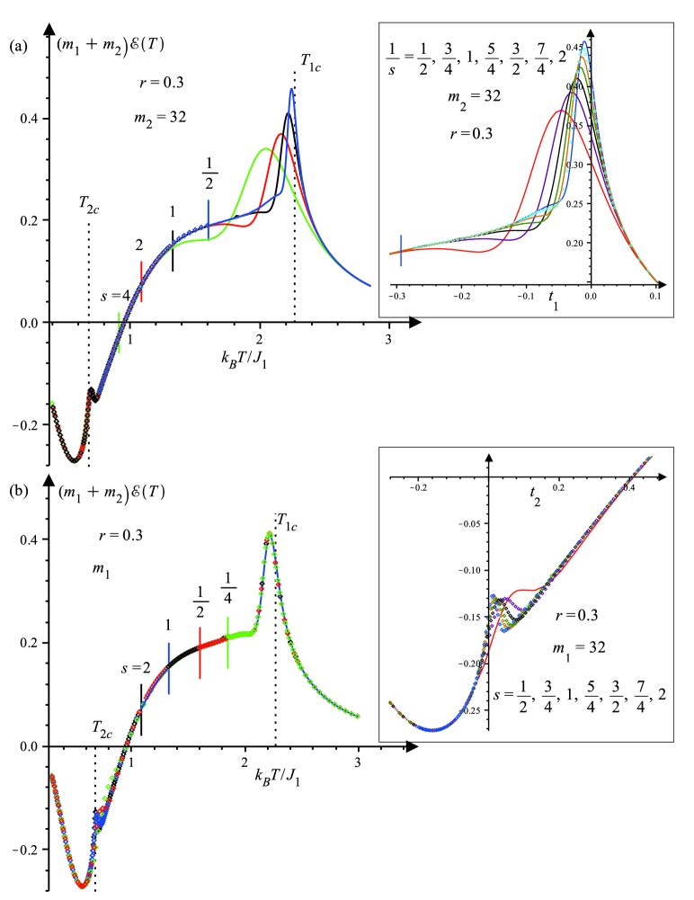
Figure 9: (Color online) The rescaled enhancement $(m_{1}+m_{2}){\cal E}(T)$ for $r=0.3$ is plotted for $m_{2}=32$, and $m_{1}=8,16,32,64$ in (a) showing that data collapses occur near $T_{2c}$. The framed inset shows more detail near $T_{1c}$ as a function of $t_{1}=(T/T_{1c})-1$. In (b) the plots are for $m_{1}=32$, and $m_{2}=8,16,32,64$. Now the data become independent of $m_{2}$ near $T_{1c}$. The behavior near $T_{2c}$ is plotted versus $t_{2}=(T/T_{2c})-1$ in the frame.

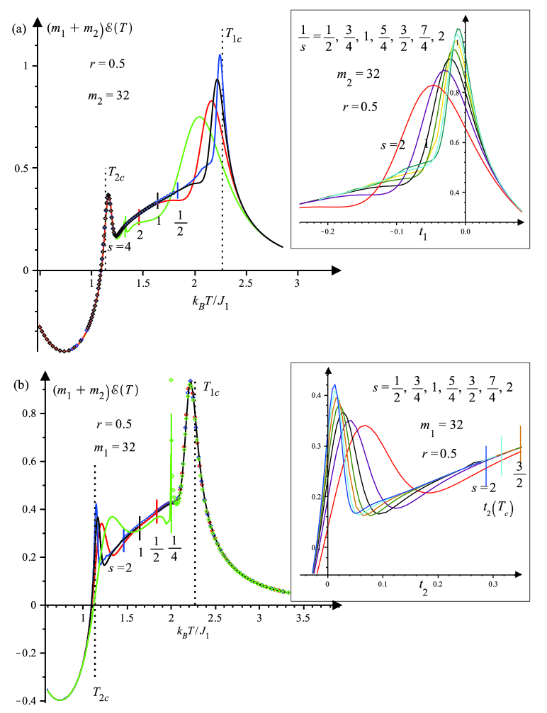
Figure 10: (Color online) Plots of the rescaled enhancement $(m_{1}+m_{2}){\cal E}(T)$ for $r=0.5$ as in Fig. 9. The short vertical lines denoted the positions of $T_{c}(s)$.

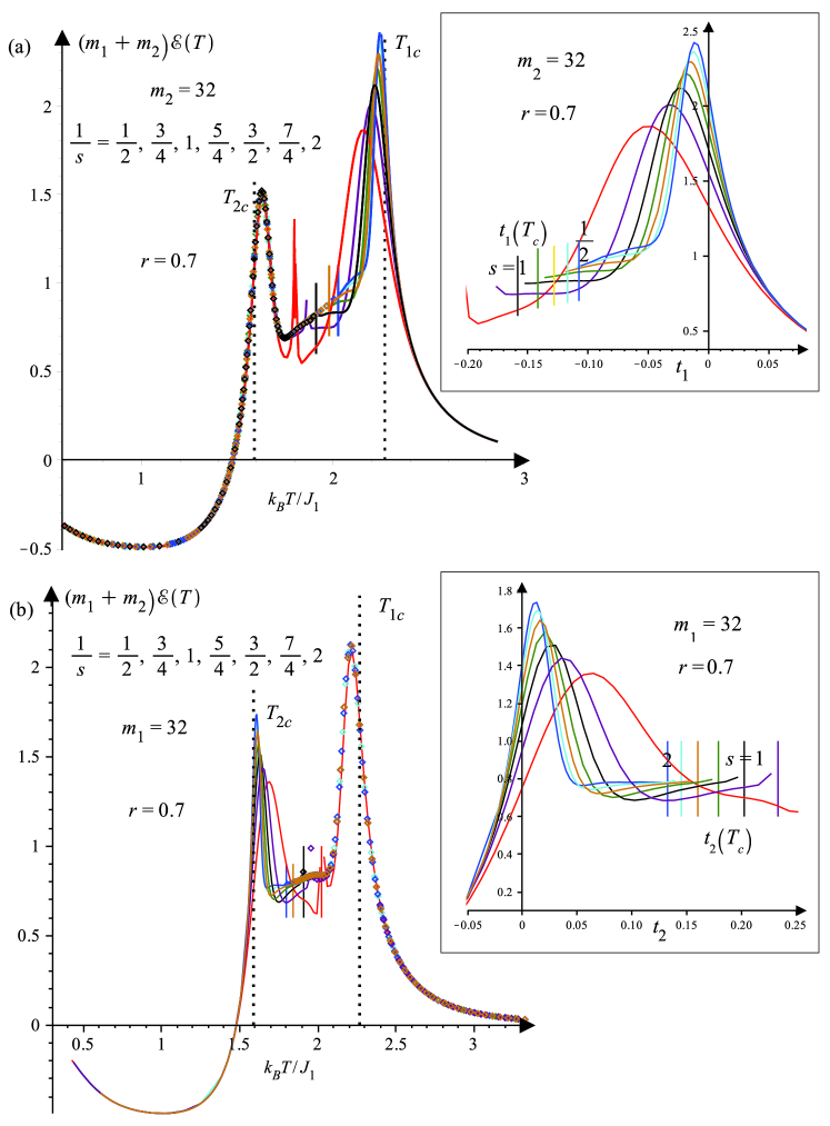
Figure 11: (Color online) The rescaled enhancements $(m_{1}+m_{2}){\cal E}(T)$ for $r=0.7$: (a) for $m_{2}=32$, and $m_{1}=8n$ for $n=2,3,\cdots,7,8$; data collapse occurs near $T_{2c}$, while the frame shows details near $T_{1c}$ vs. $t_{1}$; (b) for $m_{1}=32$, and $m_{2}=8n$ for $n=2,3,\cdots,7,8$; the plots near $T_{1c}$ are now independent of $m_{2}$, while the behavior near $T_{2c}$ is shown in the frame.

Inspection of Figs. 9-11 demonstrates that as $m_{1}$ increases, the upper maxima approach $T_{1c}$ from below, and grow steadily in height resembling the corresponding specific heats shown in Fig. 2(a). By contrast, the lower rounded peaks of the rescaled enhancements, though much smaller, lie above the limit $T_{2c}$ and similarly grow in height as $m_{2}$ increases. These observations in comparison with Figs. 2(a), 3, and 4 and the subsequent scaling analyses utilizing relations (10), (15) and (21), strongly suggest the presence of a logarithmic dependence of the peak heights on $m_{1}$ for $T>T_{c}$, but on $m_{2}$ for $T<T_{c}$.

To investigate this issue concerning the vicinities of $T_{1c}$, and $T_{2c}$ further, we have calculated the critical values of the rescaled enhancements, namely, $(m_{1}+m_{2}){\cal E}(T_{1c})$ and $(m_{1}+m_{2}){\cal E}_{2c}(T_{2c})$, for $r=0.3$, $0.5$, and $0.7$ and for eight specific values of $m_{1}$ or $m_{2}$, respectively, in the range 8 up to 64. The results are plotted vs. $\ln m_{1,2}$ in Fig. 12.

Evidently the data are well described by the form

$$(m_{1}+m_{2}){\cal E}^{\pm}_{c}(m)\simeq{\cal B}^{\pm}(r)\ln[m/m^{\pm}_{0}(r)],\quad T_{ic}\gtrless T_{c},$$

(23)

where fitted values of the amplitudes, ${\cal B}^{\pm}(r)$, and offsets, $m^{\pm}_{0}(r)$, for the upper and lower maxima, are set out in Table I. Both the amplitude and the offset appear to vary exponentially rapidly with $r$ in the region, say $0.2<r<0.8$.

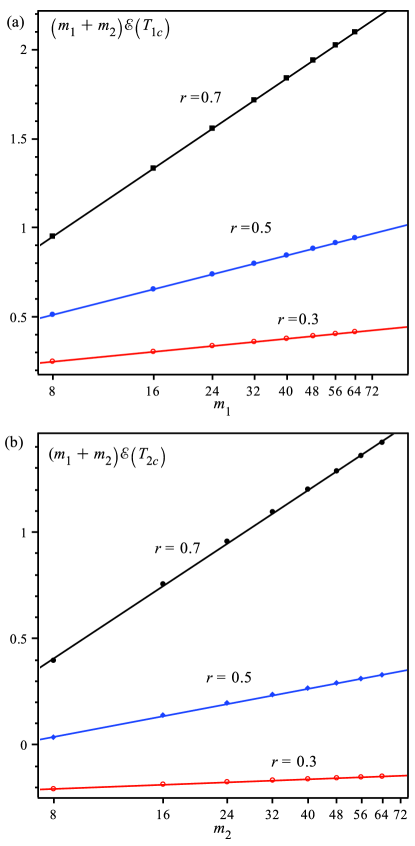
Figure 12: (Color online) The rescaled enhancement $(m_{1}+m_{2}){\cal E}(r;T)$ evaluated at the limits (a) $T_{1c}$ and (b) $T_{2c}$ for three values of $r$, plotted versus $\ln m_{1}$ and $\ln m_{2}$, respectively. The linear fits are as specified in (23) and Table I.

	$r=0.3$	$r=0.5$	$r=0.7$
$\quad{\cal B}^{+}(r)\quad$	0.0800	0.2071	0.5115
$\quad m^{+}(r)\quad$	0.358	0.677	1.427
$\quad{\cal B}^{-}(r)\quad$	0.0282	0.1405	0.4913
$\quad m^{-}(r)\quad$	$12600$	6.13	3.50

Table 1: Amplitudes and offsets for the rescaled enhancements at $T_{1c}$ and $T_{2c}$ as shown in Fig. 12. Note that the very large value $m^{-}(0.3)=12600$ combined with the small value for ${\cal B}^{-}(0.3)$ yields ${\cal B}^{-}\ln(8/m^{-}_{0})=-0.207$ which agrees with the plot in Fig. 12(b).

Beyond the relatively slow logarithmic growth of the enhancement maxima at both limits, $T_{1c}$ and $T_{2c}$, it is reasonable, on the basis of Figs. 9-11, to speculate as to the limiting behavior of ${\cal E}(J_{1},J_{2};m_{1},m_{2};T)$ in the three regions: above, below, and in-between $T_{1c}$ and $T_{2c}$.

It seems natural to propose, first, a logarithmic form in $t_{1}$ and $t_{2}$, say,

$$(m_{1}+m_{2}){\cal E}(T)\hskip 60.00009pt$$ (24)

$$\quad\approx\,\mathcal{A}^{+}(r)\ln|t_{1}|+\mathcal{C}^{+}(r), t_{1}>0$$ if ,

$$\quad\approx\,\mathcal{A}^{-}(r)\ln|t_{2}|+\mathcal{C}^{-}(r), t_{2}<0$$ if ,

as valid above and below $T_{1c}$ and $T_{2c}$. Since the limit $r\to 1$ corresponds to a uniform Ising square lattice with a symmetric logarithmic singularity, as in (1), it might be tempting to guess that the amplitudes ${\cal A}^{+}(1)$ and ${\cal A}^{-}(1)$, and the backgrounds, ${\cal C}^{+}(1)$ and ${\cal C}^{-}(1)$, are equal; but that would surely go beyond what our numerical evidence might support.

As regards the intermediate regions, however, a very different behavior seems implied. Thus, ignoring the logarithmic spikes, for $T$ between $T_{1c}$ and $T_{2c}$ and for $r$ not too large, the enhancement $(m_{1}+m_{2}){\cal E}(r;T)$, appears to increase smoothly and monotonically. Indeed the large $s^{-1}$ plots are almost linear. On extrapolating this linearity up to $T_{1c}$ and down to $T_{2c}$ in a nonsingular fashion, one finds clear numerical limits for $t_{1}\to 0^{-}$ and $t_{2}\to 0^{+}$. Specifically, the numerical evidence suggests the increasing values

$$(m_{1}+m_{2}){\cal E}^{+}_{c}(r)\simeq 0.27,\quad 0.56,\quad 1.3,$$

$$(m_{1}+m_{2}){\cal E}^{-}_{c}(r)\simeq -0.20,\quad 0.15,\quad 0.75,$$ (25)

for $r=0.3$, $0.5$, and $0.7$, respectively. While further numerical studies might reduce the uncertainties of these approximate estimates, a firm theoretical base unfortunately seems beyond current reach.

V SUMMARY : 2D-1D ISING vs. 3D-0D SUPERFLUID HELIUM

In this Section we will summarize our study of connectivity and proximity in two-dimensional alternating layered Ising models and examine the relationships to the extensive studies of Gasparini and coworkersGKMD ; KMG ; PKMG ; PKMGn ; PG ; PKMGpr on coupling and proximity effects in small “boxes” of liquid helium-4 in the vicinity of the bulk, three-dimensional superfluid transition.

To start, we considered a set of strong square-lattice Ising model strips, with spin-spin interaction $J_{1}$ and finite width $m_{1}$, that in the limit $m_{1}\to\infty$ have a bulk two-dimensional Ising transition with a logarithmically divergent specific heat at a temperature $T_{1c}$. For finite $m_{1}$, however, an isolated one-dimensional strip will display only a rounded maximum at a lower temperature, say $T_{1max}$, which, for $m_{1}$ large enough, will be well described by finite-size scaling theory.Fisher ; Barber Our numerical studies explored values of $m_{1}$ up to 64.

This situation may be compared with three-dimensional but finite-sized, and hence zero-dimensional, “boxes” of liquid helium of linear dimension, say $L_{1}$, which in the limit $L_{1}\to\infty$ will exhibit a sharp specific heat singularity at the bulk lambda point, $T_{\lambda}$. In the experiments of Gasparini and coworkers,PKMG ; PKMGn ; PG ; PKMGpr box sizes $L_{1}=1\,\mu$m and $2\,\mu$m were examined, as described further below. But it might be noted that, on accepting a microscopic scalePKMGpr $\xi^{+}_{0}=0.143$ nm, these magnitudes of $L_{1}$ might more realistically be viewed as corresponding to $m_{1}\simeq 7,000\,$-$14,000$, values far beyond our computing capabilities.

Second, in the Ising context (as illustrated in Fig. 1) the infinite number of strong strips were connected by weak or coupling strips with interactions $J_{2}=rJ_{1}$ (with $r<1$) and width $m_{2}=sm_{1}$ [as introduced in (2)], where our exact calculations yielded explicit results for interaction ratios and relative spacings in the ranges, say, $r=0.2$ to $0.9$ and $s=0.3$ to $2.0$ (although in some cases up to $s=8$). For large enough $m_{1}$ and $m_{2}$ and small enough $r$, four new distinct temperatures (beyond $T_{1c}$) were identified in plots of the specific heats (per lattice site) of the coupled system; see Figs. 1-4. In decreasing magnitude these were

$$T_{1c}>T_{1max}>T_{c}(r,s)>T_{2max}>T_{2c},$$ (26)

where $T_{1max}$ and $T_{2max}$ locate rounded but (for $m_{1},m_{2}\gg 8$) increasingly sharp maxima, while $T_{c}(r,s)$ locates an overall or bulk critical point where the specific heat must diverge logarithmically. However, the amplitude of this logarithmic singularity vanishes exponentially fastHAY with increasing $(1-r)m_{1}m_{2}/(m_{1}+m_{2})$, as indicated in the text following (2). As a consequence, the divergence soon becomes invisible on graphical plots: see Figs. 2 and 3. Finally, $T_{2c}$ represents the bulk Ising critical point for interactions $J_{2}$; consequently, when $m_{2}\to\infty$, the lower-$T$ (or weaker) maxima obey $T_{2max}\to T_{2c}$ which simply corresponds to the weaker, coupling strips become infinitely wide.

In the experimentsPKMGn ; PG ; PKMGpr a large two-dimensional lattice of the liquid helium boxes, at edge-to-edge separation $L_{2}$ (say, $=sL_{1}$) with $L_{2}=1\,\mu$m to $4\,\mu$m, was connected and, thereby, coupled to a greater or lesser degree, via, in the later experiments, a “two-dimensional helium film of thickness 33 nm.” This film corresponds, in the alternating-strip Ising model, with the weak strips that connect and couple the strong strips; in this way one might hope to identify an effective $J_{2}$ from the superfluid transition of the film, at say, $T_{s}<T_{\lambda}$: see below. In the earlier experiments,PKMGn ; PG the connection of the boxes was achieved via channels of widthPKMGn $1\,\mu$m and depth 19 nm (for $L_{1}=1\,\mu$m boxes) and of widthPKMGn ; PG $2\mu m$ and depth 10 nm (for $L_{1}=2\,\mu$m boxes); in the Ising context, this set of channels then constitutes the weak system.

Now proximity effects appear dramatically in the Ising context via the fact — clear in Figs. 2-4 and, especially, in Fig. 5 — that although an isolated and finite 1D strip must always have its specific heat peak below the corresponding bulk critical temperature,HAY namely, for the weak strips, $T_{2c}$, the lower-$T$ peaks (associated with the weak strips) are always located above $T_{2c}$. For the parameters we have used, these positive shifts amount to a few percent; more precisely, the fractional shift is close to $0.89/m_{2}$. Evidently, the shifts must be attributed entirely to the fact that the weak strips “feel,” very directly, the ordering effects of the already well ordered strong strips.

In the experiments on liquid helium, since all observed features are close to $T_{\lambda}$, we follow Gasparini and coworkers and use the temperature deviation variable

$$\dot{t}=(T/T_{\lambda})-1<0\quad\text{for $T<T_{\lambda}$}.$$ (27)

Then Fig. 7 of Ref. PKMGpr, , exhibits essentially the same proximity effect! Specifically, while the specific heat maximum of an isolated helium film occurs at $\dot{t}_{2max}^{\infty}\simeq-2.4\times 10^{-3}$, the presence of already superfluid boxes of size $L_{1}=2\,\mu$m spaced edge-to-edge at $L_{2}=4\,\mu$m apart raises the maximum in the film’s specific heat to $\dot{t}_{2max}\simeq-1.4\times 10^{-3}$. That amounts to a positive proximity shift of $0.1$% of $T_{\lambda}$. While this is quite small, the precision of the experiments is so great that the effect is beyond question.

Another aspect of the proximity (not investigated directly in the Ising strip system) is evident in Fig. 8 of Ref. PKMGpr, . This shows observations of the superfluid density, $\rho_{s}(T)$, for an isolated helium film; this vanishes (discontinuously) above the corresponding lambda point at $\dot{t}_{c}=-3.0\times 10^{-3}$. On the other hand, in the presence of the $2\,\mu$m boxes separated by $4\,\mu$m the superfluid density of the connecting film is significantly enhanced. Furthermore, the transition point itself rises, by 0.12% of $T_{\lambda}$, to $\dot{t}_{c}=-1.8\times 10^{-3}$. Even more dramatic are the observations of $\rho_{s}(T)$ shown in Fig. 16 of Ref. PKMGpr, (or Fig. 4 of Ref. PG, ): in the presence of $L_{1}=2\,\mu$m boxes spaced closer at $L_{2}=2\,\mu$m edge-to-edge, the transition point of the film rises to $\dot{t}_{c}=-18\times 10^{-3}$, “a full decade closer to $T_{\lambda}$” as Perron et al.PKMGpr comment.

Beyond the proximity effects discussed, we have studied within the model of alternating Ising strips, the enhancements of the maxima caused by the coupling between the strips. These effects can be made evident by first noting that merely on the basis of finite-size scaling the specific heats should display rounded maxima near to but, for the upper or strong maxima, displaced below $T_{1c}$ — the bulk critical point of the 2D Ising model with interactions $J_{1}$. To detect the effects of the coupling, therefore, we have defined in (22) the net enhancement, ${\cal E}(T)$, by subtracting the expected (and knownHAY ; HAYFisher ) rounded maximum of an isolated strip (for given $m_{1}$). The definition (22) also includes deductions related to the lower maxima associated with the weaker strips; but these are of negligible magnitude in the vicinity of $T_{1c}$.

Then, as seen clearly in Figs. 7-11, there are significant residual contributions, due to the coupling, that increase or enhance the upper rounded maxima well above the pure scaling contributions. Further numerical explorations (see Figs. 9-12) then demonstrate that the overall net enhancement can, at least approximately, be decomposed in to a finite background piece of order $1/(m_{1}+m_{2})$ plus quite narrow although rounded peaks near $T_{1c}$ and $T_{2c}$ of magnitude of order $\ln(m_{i})/(m_{1}+m_{2})$ for $i=1,2$, respectively. The location of the upper peaks is, in all cases, given roughly by

$$t_{1max}\approx-0.893/m_{1}.$$ (28)

At this point these various conclusions, while in our view fully convincing, lack support from exact asymptotic theory. Nevertheless, it is certainly clear theoreticallyFisherFerd that the regularly spaced seams or grain boundaries along which the strong and weak strips meet, must give rise to corrections asymptotically of order at least $1/(m_{1}+m_{2})$.

For the experiments on liquid helium the analogous enhancement effects arising from the coupling are evident in Figs. 13 and 18 of Ref. PKMGpr, (and Fig. 3 of Ref. PG, ). Specifically, Fig. 13 for $L_{1}=1\,\mu$m boxes coupled via channels (of width $1\,\mu$m, depth 19 nm, with $L_{2}=1\,\mu$m) shows a relatively narrow but well determined specific heat peak needed to correct for the lack of scaling which is, otherwise, expected for well isolated boxes of this size. Then, Fig. 18 shows an enhancement form of quite similar shape and magnitude when $L_{1}=2\,\mu$m boxes at separation $L_{2}=2\,\mu$m are coupled via a 33 nm film. The enhancement here, in fact, increases the peak height by about 9% (relative to uncoupled boxes) while the peak location is again below $T_{\lambda}$ at approximately $\dot{t}_{max}=-20\times 10^{-6}$. If this displacement is compared with the Ising result (28) one might conclude that an appropriate match would require $m_{1}$ of order $40,000$; this is several times larger than the previous estimate of an appropriate value of $m_{1}$ (in the third paragraph of this Section). This difference might, however, be related mainly to the distinctly different dimensionalities entailed in the helium and Ising systems; that, in turn, along with the different dimensionality of the order parameter, is an effect hard to guess.

Finally, however, it is clear that while the behavior of the alternating layered Ising model reflects quite directly many of the novel proximity and coupling features uncovered in the striking experiments of Gasparini and coworkers for liquid heliumPKMGn ; PG ; PKMGpr the quantitative features differ considerably. More specifically, while the range of relative separations, $s=m_{2}/m_{1}$, explored numerically compares well with that relevant in the experiments (where, essentially, $L_{2}/L_{1}=1$ or $2$), the strength ratio $r$, which in our study has been confined to $r<0.9$, should be much closer to unity to match the experimental data. One might, for example, use the observed values of the superfluidity onset temperatures relative to $T_{\lambda}$ and derive an estimate for $r$ from the ratios of $T_{c}(r,s)/T_{1c}$, etc. Similarly, one might regard the observed maximum of the specific heat of an isolated 33 nm helium film as providing an estimate of $T_{2c}$ in the model and hence of the ratio $r=T_{2c}/T_{1c}=J_{2}/J_{1}$. Implementing these suggestions leads to values of $(1-r)$ of order $3\times 10^{-3}$. In this regime of very small $(1-r)$, the separate rounded peaks associated with $T_{1c}$ and $T_{2c}$ may, indeed, not be realized, as already clear for $(1-r)=0.1$ in Fig. 2. Clearly, the experiments represent a rather different region of the underlying parameter space than that which we have explored.

- (1) F. M. Gasparini, M. O. Kimball, K. P. Mooney, M. Diaz-Avila, Finite-size Scaling of 4He at the Superfluid Transition, Rev. Mod. Phys. 80, 1009–1059 (2008).
- (2) M. E. Fisher, Theory of Critical Point Singularities, Sec. 5, Proc. 51st Enrico Fermi School, Varenna, Italy: Critical Phenomena, ed. M. S. Green, Academic Press, New York, 1–99 (1971).
- (3) M. N. Barber, Finite Size Scaling in Phase Transitions and Critical Phenomena, vol. 8, eds. C. Domb and J. L. Lebowitz, Academic Press, London, 145–266 (1983).
- (4) M. O. Kimball, K. P. Mooney, and F. M. Gasparini, Three-Dimensional Critical Behavior with 2D, 1D, and 0D Dimensionality Crossover: Surface and Edge Specific Heats, Phys. Rev. Lett. 92, 115301 (2004).
- (5) J. K. Perron, M. O. Kimball, K. P. Mooney, and F. M. Gasparini, Lack of Correlation-length Scaling for an Array of Boxes, J. Phys.: Conf. Ser. 150, 032082 (2009).
- (6) J. K. Perron, M. O. Kimball, K. P. Mooney, and F. M. Gasparini, Coupling and Proximity Effects in the Superfluid Transition in 4He Dots, Nature Physics 6, 499–502 (2010).
- (7) M. E. Fisher, Superfluid Transitions: Proximity Eases Confinement, Nature Physics 6, 483–484 (2010). News & Views: Comment on Perron et al. PKMGn
- (8) J. K. Perron, and F. M. Gasparini, Critical Point Coupling and Proximity Effects in 4He at the Superfluid Transition, Phys. Rev. Lett. 109, 035302 (2012).
- (9) J. K. Perron, M. O. Kimball, K. P. Mooney and F. M. Gasparini, Critical Behavior of Coupled 4He Regions near the Superfluid Transition, Phys. Rev. B 87, 094507 (2013).
- (10) H. Au-Yang, Criticality in Alternating Layered Ising Models: II. Exact Scaling Theory. Preprint arXiv:1306.5833.
- (11) B. Kaufman, Crystal Statistics. II. Partition Function Evaluated by Spinor Analysis, Phys. Rev. 76, 1232–1243 (1949).
- (12) A. E. Ferdinand and M. E. Fisher, Bounded and Inhomogeneous Ising Models I. Specific Heat Anomaly of a Finite Lattice, Phys. Rev. 185, 832–846 (1969).
- (13) M. E. Fisher, Aspects of Equilibrium Critical Phenomena, J. Phys. Soc. Japan (Suppl.) 26, 87–93 (1969): see Sec. 7, Eqns. (28)-(30). See also Ref. KardarBerker, .
- (14) B. M. McCoy and T. T. Wu, “The Two-Dimensional Ising Model,” Harvard Univ. Press, Cambridge, Mass. (1973).
- (15) H. Au-Yang and B. M. McCoy, Theory of Layered Ising Model: Thermodynamics, Phys. Rev. B 10, 886–891 (1974).
- (16) J. R. Hamm, Regularly Spaced Blocks of Impurities in the Ising Model: Critical Temperature and Specific Heat, Phys. Rev. B 15, 5391–5411 (1977).
- (17) H. Au-Yang and M. E. Fisher, Bounded and Inhomogeneous Ising Models II. Specific Heat Scaling Function for a Strip, Phys. Rev. B 11, 3469–3487 (1975). See also Ref. WuHuIzmailian, .
- (18) M. E. Fisher, and A. E. Ferdinand, Interfacial, Boundary, and Size Effects at Critical Points, Phys. Rev. Lett. 19, 169–172 (1967).
- (19) M. Kardar and A. N. Berker, Exact Criticality Condition for Randomly Layered Ising Models with Competing Interactions on a Square Lattice, Phys. Rev. B 26, 219–226 (1982).
- (20) M.-C. Wu, C.-K. Hu, N. Sh. Izmailian, Universal Finite-Size Scaling Functions with Exact Nonuniversal Metric Factors, Phys. Rev. E 67, 065103(R) (2003).