Study of unconventional superfluid phases and the phase dynamics in spin-orbit coupled bose system

Abstract

We study the phase distribution and its dynamics in spin-orbit coupled two component ultracold Bosons for finite size system. Using an inhomogeneous meanfield analysis we demonstrate how phase distribution evolves as we tune the spin-orbit coupling $\gamma$ and $t$, the spin-independent hopping. For $t>>\gamma$ we find the homogeneous superfluid phase. As we increase $\gamma$, differences in the phases of the order parameter grows leading to twisted superfluid phase. For $t\sim\gamma$ competing orderings in the phase distribution is seen. At large $\gamma$ limit a Ferro-Magnetic stripe ordering appears along the diagonal. We explain that this is due to the frustration bought in by the spin-orbit interaction. Isolated vortex formation is also shown to appear. We also investigate the possible collective modes. In deep superfluid regime we derive the equation of motion for the phases following a semi-classical approximation. Imaginary frequencies indicating the damped modes are seen to appear and the dynamics of lowest normal modes are discussed.

I Introduction

The recent advancement in optical lattice experiments to investigate the idealized strongly correlated many body system has initiated a great interest among the condensed matter community morsch . Starting from mimicking simple tight binding Hamiltonian in a periodic lattice, it can now create more complex situations seen in real materials. Creation of artificial abelian or non-abelian gauge fields, density-density interaction are some of them to mention daliberd ; linrmp . Experimental realization of Mott-Insulator to Superfluid transition for ultracold bosons Greiner1 ; Orzel1 in such system became a paradigm of itself. Recently there has been experimental realisation to simulate tunable spin-orbit coupling in neutral bosons in optical latticesopapers1 ; ylin . This has been remarkable because it is known that for real material spin-orbit coupling is in essential an intrinsic toprev1 properties of the material and could not be controlled. The spin-orbit interaction can change the physical properties of the system dramatically. In optical lattice the spin-orbit coupling is achieved by Raman laser induced transitions between the two internal states of a neutral bosonic atom. The resulting spin-orbit interaction could be purely Rashbha rashbha type or Dresselhaus dresselhaus type or suitable combination of both.

The result of such spin orbit interaction has been studied extensively recently victor1 ; arun1 ; cw1 ; grab-sarma ; chunjiwang ; ychang . In the Mott regime it is shown to support exotic magnetic textures, such as vortex crystals and skyrmion lattice victor1 ; arun1 ; cw1 . The signature of the Mott-Insulator to Superfluid transition has been shown to be associated with precursor peaks in momentum distributions saha1 ; sinha1 ; issacson1 ; man-saha-sen . Various other equilibrium and non-equilibrium dynamics has also been analyzed which could have interesting experimental signatures arun2 . Boson fractionalisation has also been proposed and formation of twisted superfluid phases has been noticed as a result of spin-orbit interaction man-saha-sen ; panahi . It may be mentioned that for the fermionic case interesting many body dynamics has also been observed vi1 .

The Mott-Insulator to Superfluid transition is well captured by Bose-Hubbard model fisher1 ; sachdev1 ; jaksch1 . There are already a large number of work done to investigate the low energy properties of such Bose-Hubbard model sesh1 ; trivedi1 ; sengupta1 ; dupuis1 ; hrk1 . However much of these work was mainly aimed at investigating the systems which are thermodynamically large and in weak couple regime. In this work we look into the effect of spin-orbit interaction of two component bosons in strong coupling limit for different finite size systems. We are motivated to look into microscopic manifestation of the spin-orbit interaction and various ramifications of superfluid order parameter for different system size and different parameter regime. For this we employ Gutzwiller projected inhomogeneous meanfield treatment hrk1 which seems to be pertinent for such small system size. We work in the strong coupling limit where the Hubbard interaction is the highest energy scale of the problem. This limit enables us to take the number of states in the Gutzwiller projected state to be necessary minimal. Below we describe our plan of work.

In section I, we begin by giving a detail analysis of the meanfield procedure and obtain the phase diagram for MI-SF transition. Following this, we look into the phases and magnitude of the SF order parameter in superfluid regime. We show that the phases and the magnitude of the SF order parameter respond non-trivially as the parameters are varied. We find that when $t>>\gamma$, the SF phase is described by a homogeneous superfluid where the magnitude and the phases of the up spins are spatially uniform. For intermediate values of $t$ and $\gamma$ we find that the phases and the amplitudes of both the spins are inhomogeneous and shows interesting nontrivial pattern. Depending on the relative strength it could be superposition of local homogeneous phases and patches where the phases form a spiralling pattern. For the limit $\gamma>>t$, the phases of the order parameter develops a Ferromagnetic order along the diagonal direction followed by periodic modulations of magnitude of the SF order parameter. We explain that this is due to inherent frustration brought in by the spin-orbit interaction.

In section II, we study the fluctuations around the meanfield configuration and investigate into the lowest possible excitations. In section III, we study the dynamics of phases inside the deep SF regime. Assuming that the phases of the order parameters are the low energy degrees of freedom in this regime, we deduce the Lagrange-Equation of motion for it. We find the normal modes. It appears that due to the constrained collective motion imaginary frequency appears signifying damped vibration. We also look at the nature of lowest normal modes of the vibrations.

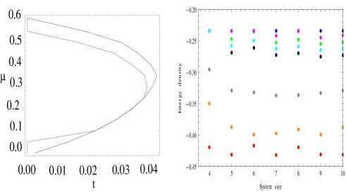
Figure 1: In the left panel we have shown the MI-SF transition for $\lambda=0.6,\Omega=0.01$ in $\mu-t$ plane. The blue line denotes the transition for $\gamma=0$ and the red line denotes $\gamma=0.04$. In the right panel we have plotted the energy density per plaquette with various system sizes for different parameter values. The various color represents various set of ($\gamma,t$) which are explained in the text.

II Meanfield study

As already mentioned in this work we study a spin-orbit coupled two component bosons in square lattice. The Hamiltonian for such a system can be written as $H=H_{0}+H_{1}$, where $H_{0}$ and $H_{1}$ are given by ylin ; man-saha-sen ,

$$H_{0}=\sum_{ia}-\mu n_{ia}+Un_{ia}(n_{ia}-1)+\lambda U\sum_{i}n_{i1}n_{i2}$$

$$-\sum_{\langle ij\rangle_{a}}t_{a}b^{\dagger}_{ia}b_{ja},~{}~{}~{}H_{1}=i\gamma\sum_{i}\Psi^{\dagger}_{i}\hat{z}.(\vec{\sigma}\times\vec{d}_{ij})\Psi_{j}$$

$$+\sum_{i}\left(\delta\Psi^{\dagger}_{i}\sigma_{y}\Psi_{i}-\Omega\Psi^{\dagger}_{i}\sigma_{z}\Psi_{i}\right)$$ (1)

Here $\Psi_{i}=\left(b_{i1},b_{i2}\right)$. In the above Hamiltonian $\mu$ represents the chemical potential, $\Omega$ is the Zeeman shift between the two species, $U$ is the intraspecies interaction and $\lambda$ is the on site interspecies interaction. For the meanfield analysis we take the Gutzwiller variational wave function $|\Psi\rangle=\prod_{i}|\psi_{i}\rangle$, where $|\psi_{i}\rangle$ is the wave function at a given site ’$i$’. $|\psi_{i}\rangle$ is given by $|\psi_{i}\rangle=\sum_{m,n}f_{m,n}|mn\rangle$. As we work in a strong coupling limit where $U$ is much larger that $t$ and $\gamma$, it is sufficient to take states upto 2 particle at a given site. The meanfield order parameter is defined as, $\Delta_{ia}=\langle\psi_{i}|b_{ia}|\psi_{i}\rangle$. The expression for $\Delta_{ia}$ in terms of $f_{mn,i}$ are given below,

$$\Delta_{i1}=f_{10,i}f^{*}_{00,i}+f_{11,i}f^{*}_{01,i}+\sqrt{2}f_{20,i}f^{*}_{10,i}$$

$$\Delta_{i2}=f_{01,i}f^{*}_{00,i}+f_{11,i}f^{*}_{10,i}+\sqrt{2}f_{02,i}f^{*}_{01,i}$$ (2)

The first part of the Hamiltonian in Eq.(1) contains the on site interactions and we call it $H_{at}$ which given by,

$$\langle H_{at}\rangle_{i}=-\mu_{1}\Big{(}|f_{10,i}|^{2}+|f_{11,i}|^{2}+2|f_{20,i}|^{2}\Big{)}+\lambda U|f_{11,i}|^{2}-$$

$$\mu_{2}\Big{(}|f_{01,i}|^{2}+|f_{11,i}|^{2}+2|f_{02,i}|^{2}\Big{)}+2U\Big{(}|f_{20,i}|^{2}+|f_{02,i}|^{2}\Big{)}~{}~{}~{}$$ (3)

A generic term in $H_{1}$ can be written as $b^{\dagger}_{i,\alpha}b_{j,\beta}$. The meanfield decomposition of it is given by,

$$b^{\dagger}_{i,\alpha}b_{j,\beta}=\Delta^{*}_{i\alpha}b_{j\beta}+\Delta_{j\alpha}b^{\dagger}_{i\beta}-\Delta^{*}_{i\alpha}\Delta_{j\beta}$$ (4)

After we substitute Eq.(3), Eq.(4) in Eq.(1) and use Eq.(2) we can write the meanfield decomposed Hamiltonian as,

$$H=\sum_{i}\chi^{\dagger}_{i}F_{i}(\mu,\lambda,\Delta_{j,\alpha},t,\gamma)\chi_{i}$$ (5)

where $\chi_{i}=\left(f_{00,i},f_{10,i},f_{01,i},f_{11,i},f_{20,i},f_{02,i}\right)$. The problem then reduces to diagonalizing the matrix $F_{i}$ at every site self consistently. The Hamiltonian in Eq.(5 is still a coupled problem. We notice that in the presence of spin-orbit coupling $\Delta_{i}$ can not be taken uniform at each site for then the spin-orbit interaction contribute nothing to the total energy. To find the meanfield solution, we start from a given random initial distribution of $\Delta_{i}$ at each site $i$ diagonalize the $F_{i}(\mu,\lambda,\Delta_{j,\alpha},t,\gamma)$ at each site. We then calculate the new set of $\tilde{\Delta}_{i}$ corresponding to the minimum eigenvalue of $F_{i}$. The resulting $\tilde{\Delta}_{i}$’s are fed back into Eq.(5) until $\Delta_{i}$ becomes equals to $\tilde{\Delta}_{i}$ at each site $i$. We do this procedure for approximately $10^{4}$ random configurations and take the configurations of $\tilde{\Delta}_{i}$ which corresponds to the global minima. In the Fig.(1) left panel, we show the phase diagram for the MI-SF transitions. In the right panel of Fig.(1), we have plotted the energy density per site with the system size for various set of parameter . We find that finite size minimization brings significant variations in the energy density with the system size. The various color represents various set of parameters ($\gamma,t$). Red represents (0.1,0.02), blue represents (0.02,0.04), green represents (0.03,0.04), black is for (0.04,0.04), gray is for (0.06,0.04), orange denotes (0.08,0.04) magenta denotes (0.025,0.04) and cyan is for (0.035,0.04). This color scheme is maintained for all the figures that will be used later. In the following we discuss the textures of the order parameter $\Delta_{ia}$ for different values of $t$ and $\gamma$.

II.1 Numerical results

First we discuss the regime when $t>>\gamma$ followed by the regime where $t\sim\gamma$. Lastly we discuss the regime where $\gamma>>t$.

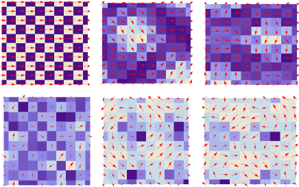
Figure 2: Magnitude and phase of the order parameter is plotted at each site. The arrows represent the phases and the color represent the magnitude of the order parameter $\Delta_{i}$. The upper panel denotes phase and magnitude for $\Delta_{1}$ and the lower panels are for $\Delta_{2}$. The left panels denotes the result for $\gamma=0.02,t=0.04$. The middle panels are for $\gamma=0.025,t=0.04$ and the right panels are for $\gamma=0.03,t=0.04$.

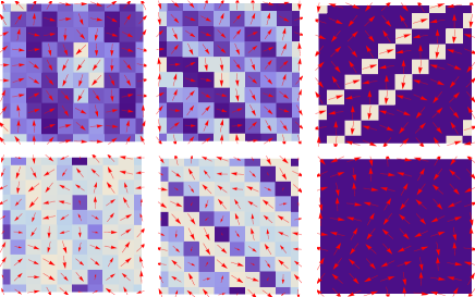
Figure 3: The distribution of phases and the order parameter as explained in Fig.(2). Here the left panels represent the result for $\gamma=0.035,t=0.04$, the middle panels represent $\gamma=0.04,t=0.04$ and the right panels represent $\gamma=0.06,t=0.04$.

II.1.1 Meanfield results when $t$ is large compared to $\gamma$.

In Fig.(2) we present the resulting distributions of phases and the magnitude of the order parameter $\Delta$. The arrows represents the phases and the background color represents the relative magnitudes of the order parameters. The dark color represents greater magnitude. The upper panel is for $\Delta_{1}$ and the lower panel is for $\Delta_{2}$. In the extreme left panel the result is shown for $t=0.04,\gamma=0.02$. We find that the distribution of phases $\Delta_{1}$ are ordered and spatially uniform while that of $\Delta_{2}$ is disordered. The magnitudes of $\Delta_{1}$ shown form a two sublattice structure, however there are degenerate solutions with spatially uniform magnitude. It is clear that the two sublattice structure is the result of spin-orbit interaction. Also we have $\langle\Delta_{1}\rangle>>\langle\Delta_{2}\rangle$. The above textures is understood easily as for the presence of $\Omega$, the system is favoring the condensation of species 1 which resembles the homogeneous superfluid. The middle panel of Fig.(2), represents the result for $t=0.04,\gamma=0.03$. We observe that the phases are no longer uniform leading to twisted superfluid phase  panahi . We observe the reduction of the ordered pattern of $\Delta_{1}$ and onset of diagonal ordering. The magnitude of $\Delta_{1}$ are also random. The $\Delta_{2}$ also shows signature of diagonal ordering. The competition of ordering along the two diagonal shows the signature of large vortices as seen in the moddlelower panal in Fig.(2).

II.1.2 $t$ and $\gamma$ is comparable

The phase textures for this regime could be described as follows. We find a competition between local ferro magnetic alignment for nearest $\Delta_{i}$’s and the ferromagnetic(FM) ordering along the diagonal neighbors. The FM ordering for the neighbors results from direct hopping. Where as the ferromagnetic ordering along the diagonal is due to the spin-orbit coupling as explained in next section. In Fig.(3), left panel represents the phase distribution for $\gamma=0.035,t=0.04$, middle panel is for $\gamma=0.04,t=0.04$ and the right panel is for $\gamma=0.06$. We notice that the minimum energy configuration presented here is not unique. There are many degenerate configurations with identical energy. However the quantum fluctuations would pick the global minima. For examples, in Fig.(3), we find the onset of density modulations and no vertex formations. There are degenerate meanfield solutions with completely random density distribution with isolated vertex formations.

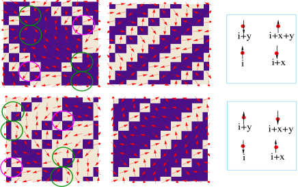
Figure 4: The distribution of phases and the order parameter as explained in Fig.(2) and (3). The left and the middle panal is drawn for $\gamma=0.1,t=0.02$. These represent the degenerate meanfield configuration. We see that the left panal contains vertex and antivertex. The green circle contains the vertex configurations and the pink circle contains antivertex. In the right panel we have shown the spin-orbit coupled hopping processes for up-spin starting from site $i$ in anti-clockwise direction.

II.1.3 $t$ is small and $\gamma$ is large

In this regime we notice that the phases forms a ferromagnetic alignment along the diagonal. The magnitude of the order parameter are also seen to be modulated. In Fig.(4), we present the distribution for the phases and the magnitude of order parameter for $\gamma=0.1,t=0.02$. We see that ferromagnetic ordering of phases along the diagonal is common. While in the left panel FM ordering happens for both the diagonal, for the middle panel it happens for only (1,1) direction. In the left panel isolated vertex victor1 and anti vertex is seen to appear. To understand the phase distribution in this regime it may be useful to consider an elementary square plaquette and consider the meanfield Hamiltonian for it. Let us consider the hopping of an up spin under spin-orbit coupling via the sites $i$, $i+x$, $i+x+y$ and $i+y$ in anti-clockwise direction as shown in the right upper panel in fig 4. The meanfield decomposition put the following constraints on the phases,

$$\theta_{i,1}-\theta_{i+x,2}=\pm\pi,~{}~{}\theta_{i+x,2}-\theta_{i+x+y,1}=\frac{\pi}{2},$$

$$\theta_{i+x+y,1}-\theta_{i+y,2}=0,~{}~{}~{}\theta_{i+y,2}-\theta_{i,1}=-\frac{\pi}{2}$$ (6)

The above set of equations do not have simultaneous solutions for all the parameters. One may eleminate $\theta_{i+x,2}$ (and $\theta_{i+y,2}$ ) from the 1st and 2nd (and 3rd and 4th) to solve for $\theta_{i,1}$ and $\theta_{i+x+y,1}$ to obtain that they are equal, the numerical outcome seems to conform this. It then poses an ill-defined equation for $\theta_{i+x,2}$ (and $\theta_{i+y,2}$ ) which is fixed to minimize the plaquette energy. The ratio of average plaquette energy obtained from numerics to that obtained by minimizing a single plaquette is 0.94 which is satisfactory. In recapitulation we have shown within meanfield how the twisted superfluid phase appears as we gradually tune the parameter $t$ and $\gamma$ for a tight binding Hamiltonian. We have shown the onset of density modulations and stripe pattern  ho-wang for the phases as the $\gamma$ is increased gradually.

III Fluctuation around the meanfield

Here we look into the fluctuations around the meanfield solutions obtained in the previous section. To take into the role of fluctuation we expand Gutzwiller coefficients  constantin $f_{mn,i}$ around its saddle point and expand it by $f_{mn,i}=\bar{f}_{mn,i}+\delta f_{mn,i}$ where $\bar{f}_{mn,i}$ represents the equilibrium values. After we substitute it in Eq.(5) we retain the terms which are quadratic in $\delta f_{mn,i}$ (and its complex conjugate). The resulting Hamiltonian then could be written as,

$$H=\Psi^{\dagger}H_{\delta}\Psi$$ (7)

where $\Psi=(\psi_{1},\psi_{2},...\psi_{r},....\psi_{N})$ and $\psi_{i}=\big{(}\psi_{ui},\psi_{di})$. Here $\psi_{ui}=(\delta f_{00,i}~{}\delta f_{10,i}~{}\delta f_{01,i}~{}\delta f_{11,i}~{}\delta f_{20,i}~{}\delta f_{02,i})$ and $\psi_{di}=\psi^{*}_{ui}$. It is clear that $H_{\delta}$ represents a $12N\times 12N$ Hermitian matrix whose eigenvalues and eigenvectors represents the collective modes. It may be noted that the substitution, $\delta f_{mn,i}=\sum_{k}u_{mn,k}e^{ikr}+v_{mn,k}e^{-ikr}$, does not simplify the problem as the $\bar{f}_{mn,i}$’s are not translational invariant. We denote the eigenvalue closer to absolute zero by $E_{0}$. The $E_{0}$ is a measure of possible Goldstone modes of the system and is shown in . We find that for $t>>\gamma$, the system always find zero energy modes. For $t\sim\gamma$, where the phases are disordered we also find similar behavior. However for $\gamma>>t$, we find that $E_{0}$ is $\sim 10^{4}$ times larger than the other parameter regime. However the $E_{0}$ scales to lower values monotonically as we increase the system size. The gradual decrease of $E_{0}$ with system size $N$ indicates that it is approaching to possible zero energy modes. The reason that $E_{0}$ for $\gamma>>t$ is larger than other cases by few thousand order is the following. For $t>>\gamma$ the uniform phase distribution always find Goldstone modes and there is no frustration in the system also. For $t\sim\gamma$, the spins are disordered and random. Thus it is easily possible to re-distribute the phases to have zero energy eigenmodes which is nearly degenerate with the original solutions. However for $\gamma>>t$, the distribution of phases and the magnitudes are governed by the frustration bought in by spin-orbit coupling. The degenerate solutions in this case as seen from Fig.(4) are not easily connected. Thus the collective excitations costs finite energy than the other cases. However as we increase the system size, we expect that the degenerate solutions are easily obtained from one other leading to zero energy mode. We also observe that the eigenvalues of the collective modes form three distinct bands. This is clear from Eq.(3). The fluctuation of $f_{2,0}$ or $f_{0,2}$ yields the bands around $U$. While the fluctuation of $f_{11}$ yields the bands around $\lambda/2$. The fluctuation of $f_{1,0},f_{0,1}$ and $f_{0,0}$ constitutes the lower bands. We denote these three bands by $E_{2},E_{1}$ and $E_{0}$ respectively. In the right panel of Fig.(5), we have plotted the band-width with the system sizes for different parameter values. In the left panel of Fig.(6) we have plotted the bandwidth of $E_{1}$ and the right panel is for $E_{0}$. It appears that for a given $t$, the bandwidth is inversely proportional to $\gamma$. Also more the value of $\gamma$, the bandwidth oscillates more with the system sizes. We notice that the bands $E_{2}$ and $E_{1}$ are symmetric but $E_{0}$ is not because of the presence of $\Omega$.

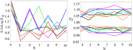
Figure 5: In the left a measure of zero energy eigenmodes $E_{0}$ due to the collective motions has been shown. In the right panel the bandwidth around $E_{2}$ has been plotted. For both the figure horizontal axis represnts the length a $N\times N$ lattice. The various colors represent various set of parameters as given in the text.

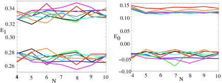
Figure 6: In the left panel the bandwidth around $E_{1}$ has been shown. The right panel is for $E_{0}$. In both the figure the horizontal axis represents the length of a $N\times N$ lattice.

IV Dynamics of the phases

Now we turn out attention to the deep inside the superfluid regime where one may neglect the fluctuations of the magnitude of the order parameter and consider the phases as the only relevant degree of freedom. Following a semi-classical approximation, we deduce the Lagrangian and the equation of motion for the phases and determine the normal modes of the vibrations. The meanfield decomposition of Eq.(1) could be written as,

$$H=\sum_{i}\mu_{\alpha,i}\langle n_{\alpha,i}\rangle+\frac{U}{2}\langle n_{\alpha,i}\rangle^{2}+\lambda U\langle n_{\alpha,i}\rangle\langle n_{\beta,i}\rangle$$

$$~{}~{}~{}~{}-\sum_{\langle ij\rangle}\left(\lambda_{ij,\alpha\beta}\Delta^{*}_{\alpha,i}\Delta_{\beta,j}+h.c\right)~{}~{}~{}~{}~{}$$ (8)

In the above $\lambda_{ij,\alpha\beta}$ denotes a general hopping parameter. The main disadvantage of Eq. (8) is that all the variables commute with each other and bear no signature of the original bosonic commutation relations. To derive Lagrangian of the phases of the order parameter $\Delta$, we follow the procedure in legget ; kivelson . Translating the original bosonic commutators to the commutation relations of the meanfield variables, we find that,

$$[n_{1},b_{1}]=-b_{1}\rightarrow[\langle n_{1}\rangle,\Delta_{1}]=-\Delta_{1}$$ (9)

Writing $\Delta_{1}=e^{i\theta_{1}}|\Delta_{1}|$ and keeping $|\Delta_{1}|$ constant we obtain,

$$[\langle n_{1}\rangle,e^{i\theta_{1}}]=-e^{i\theta_{1}}$$ (10)

Expanding $e^{i\theta_{1}}$ and keeping only the lowest order term we obtain for $\theta_{1}\rightarrow 0$, the following commutation relations,

$$[\langle n_{1}\rangle,\theta_{1}]=i,~{}~{}[\langle n_{1}\rangle^{2},\theta_{1}]=2i\langle n_{1}\rangle$$ (11)

The above procedure yields the following coupled equations to be solved for the $\frac{\partial\theta_{\alpha}}{\partial t}$ and $\frac{\langle n_{\alpha i}\rangle}{\partial t}$

$$\frac{\partial\theta_{1i}}{\partial t}=-(\mu+\Omega+\frac{U}{2})+U\langle n_{1i}\rangle+\lambda U\langle n_{2i}\rangle$$

$$\frac{\partial\theta_{2i}}{\partial t}=-(\mu-\Omega+\frac{U}{2})+U\langle n_{2i}\rangle+\lambda U\langle n_{1i}\rangle$$ (12)

Solving for $\langle n_{1i}\rangle$ and $\langle n_{2i}\rangle$ from the above two equations and substituting in the Hamiltonian, Eq. 8, we obtain the following equations,

$$H_{sh}=B_{0}\left((\frac{\partial\theta_{1i}}{\partial t})^{2}+(\frac{\partial\theta_{2i}}{\partial t})^{2}\right)+B_{1}\frac{\partial\theta_{1i}}{\partial t}+B_{2}\frac{\partial\theta_{2i}}{\partial t}$$

$$+B_{3}\frac{\partial\theta_{1i}}{\partial t}\frac{\partial\theta_{2i}}{\partial t}+F(\theta_{i1},\theta_{i2})+B_{4}$$ (13)

Where $F(\theta_{i1},\theta_{i2})$ is given in the appendix. Expressions for $A_{i}$’s are also given in the appendix. To derive the E-L equations of motion, we introduce the relative and total phase by the relation, $\theta_{1i}=\theta_{ci}+\theta_{ir},~{}~{}~{}\theta_{2i}=\theta_{ci}-\theta_{ir}$ After inserting the above change of variables we can rewrite Eq  17 as follows,

$$H_{n}=\sum_{i}T_{1}(\dot{\theta}_{ic}+\alpha_{c})^{2}+T_{2}(\dot{\theta}_{ir}+\alpha_{r})^{2}$$

$$~{}~{}~{}~{}+F(\theta_{ir},\theta_{ic})+\sum\alpha_{icr}$$ (14)

Here $T_{1/2}=2B_{0}\pm B_{3}$ Using the above equations, we write the resulting Lagrangian and the equation of motion below,

$$\mathcal{L}=\sum_{i}T_{1}(\dot{\theta}_{ic}+\alpha_{c})^{2}+T_{2}(\dot{\theta}_{ir}+\alpha_{r})^{2}-F(\theta_{ir},\theta_{ic})$$

$$\ddot{\theta}_{ic}=-\frac{\partial F(\theta_{ic},\theta_{ir})}{T_{1}\partial\theta_{ic}},~{}~{}\ddot{\theta}_{ir}=-\frac{\partial F(\theta_{ic},\theta_{ir})}{T_{2}\partial\theta_{ir}}$$ (15)

In the last equation we have deliberately omitted the inconsequential constant term $\sum\alpha_{icr}$. After simplifying the r.h.s of Eq.15 and subsequently expanding upto linear term we can rewrite it is, $\ddot{\Theta}=M\Theta$. Where for a system of $N\times N$ lattice $\Theta$ is a column matrix with $2N^{2}$ element such that $\Theta_{i}=\theta_{ic}$ and $\Theta_{N^{2}+i}=\theta_{ir}$ where $i$ runs from 1 to $N^{2}$. $M$ is a $2N^{2}\times 2N^{2}$ matrix. The eigenvalues of the matrix $M$ yields the normal modes. We find that the due to the presence of $\gamma$, the normal modes develop negative eigenvalues signifying damped modes. In fig 7 we have plotted schematically the lowest normal modes for three different regime. In all the plot the blue region denotes displacements of phases in forward direction (anti-clockwise rotation) and the white regions denotes displacements in the backward directions (clockwise rotation). The right panel denotes the case for $\gamma>>t$, the middle panel denotes $\gamma\sim t$ and the right panel is for $t>>\gamma$. In each of these panel the upper one denotes the displacement for species 1 and the lower panel describe the displacements for species 2. Looking at the upper panel we find that for the $\gamma>>t$, there is tendency of phases to move synchronously along the diagonal which is expected. However for the middle panel and the left panel there is a preferences in horizontal ordering and patches of areas vibrating in breathing modes. For the species 2, the left panel, we find similar behavior though region executing breathing modes are larger.

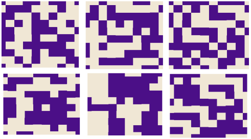
Figure 7: We have shown the nature of vibration for the lowest normal modes. In each panel the upper panales denotes $\theta_{1}$ and the lower panels are for $\theta_{2}$. The right panel denotes the the case $\gamma<t$, ($\gamma=0.02,t=0.04$). The middle panal reprensents $\gamma\sim t$, ($\gamma=0.04,t=0.04$). The right panel represent $\gamma>t$, ($\gamma=0.1,t=0.02$). The white region denotes the motion in clockwise direction and the blue region denotes motion in the anti-clockwise direction.

V Discussion

To summarize we have explored the different phases that might occur for a spin-orbit coupled bosons in the optical lattice. We have extensively studied the distribution of phases and the magnitude of order parameter for varying finite size system using an inhomogeneous meanfield analysis. We have shown that for a given $t$, as we increase the spin-orbit interaction $\gamma$, we observe the destruction of normal homogeneous superfluid phase and onset of twisted superfluid phases. At large $\gamma$ limit an interesting ordering along the diagonal appears. We have also investigated the fluctuation around the meanfield and shows the existence of Goldstone modes. The scaling of minimum energy excitations with system size has also been shown. Finally, using semiclassical approximation we derived the equation of motion for the phases and derive the normal modes of vibrations. We think that some of the results may have interesting experimental signatures in the light of recent experiments.

VI appendix

$$b_{0} = \frac{\lambda^{2}_{0}u}{2},~{}~{}b_{3}=u\lambda\lambda^{2}_{0}\left(1-\frac{1}{\lambda^{2}}\right)$$

$$b_{1} = \lambda_{0}(\frac{a_{1}}{\lambda}-a_{2})+\lambda_{0}u(a_{2}-\frac{a_{1}}{\lambda})+u\lambda\lambda_{0}(a_{1}-\frac{a_{2}}{\lambda})~{}~{}~{}~{}~{}~{}~{}$$

$$b_{2} = \lambda_{0}(\frac{a_{2}}{\lambda}-a_{1})+\lambda_{0}u(a_{1}-\frac{a_{2}}{\lambda})+u\lambda\lambda_{0}(a_{2}-\frac{a_{2}}{\lambda})~{}~{}~{}~{}~{}~{}~{}$$

$$b_{4} = -a_{1}a_{1}-a_{2}a_{2}+\frac{u}{2}(a^{2}_{1}+a^{2}_{2})+\lambda ua_{1}a_{2}$$

$$a_{1} = \mu+\omega+\frac{u}{2},~{}~{}~{}~{}~{}a_{2}=\mu-\omega+\frac{u}{2},~{}~{}~{}\lambda_{0}=\frac{\lambda}{u(\lambda^{2}-1)}$$

$$a_{1} = \lambda_{0}\left(a_{2}-\frac{a_{1}}{\lambda}\right),~{}a_{2}=\lambda_{0}\left(a_{1}-\frac{a_{2}}{\lambda}\right),$$ (16)

$$\alpha_{c}=\frac{b_{1}+b_{2}}{2(2b_{0}+b_{3})},~{}~{}\alpha_{r}=\frac{b_{1}-b_{2}}{2(2b_{0}-b_{3})},~{}\alpha_{icr}=-\alpha^{2}_{c}-\alpha^{2}_{r}$$

$$f(\theta_{i1},\theta_{i2})$$

$$=-2\gamma_{t}\sum_{\langle ij\rangle}\left(\cos(\theta_{1i}-\theta_{1j})+\eta\beta^{2}\cos(\theta_{2i}-\theta_{2j})\right)|\delta^{2}_{1}|$$

$$-2\gamma_{s}\beta\sum_{\langle ij\rangle_{x}}\left(\cos(\theta_{2i}-\theta_{1jx})-\cos(\theta_{1i}-\theta_{2jx})\right)|\delta^{2}_{1}|$$

$$+2\gamma_{s}\beta\sum_{\langle ij\rangle_{y}}\left(\sin(\theta_{1i}-\theta_{2jy})+\sin(\theta_{2i}-\theta_{1jy})\right)|\delta^{2}_{1}|$$ (17)

References

- (1) O. Morsch and M. Oberthaler, Rev. Mod. Physics, 78(1), 179, (2006).
- (2) J. Daliberd, F. Gerbier, G. Juzeliunas, and P. Ohberg, Rev. Mod. Phys. 83, 1523 (2011).
- (3) Immanuel Bloch, Jean Dalibard and Wilhelm Zwerger, Rev. Mod. Phys. 80, 885 (2008).
- (4) M. Greiner, O. Mandel, T. Esslinger, T. W. HaÈnsch, and I. Bloch, Nature 415, 39 (2002).
- (5) C. Orzel, A. K. Tuchman, M. L. Fenselau, M. Yasuda, and M. A. Kasevich, Science 291, 2386 (2001).
- (6) G. Juzeli¯unas et al., Phys. Rev. A 77, 011802(R) (2008); T. D. Stanescu, B. Anderson, and V. Galitski, ibid. 78, 023616 (2008);X.-J. Liu, X. Liu, L. C. Kewk, and C. H. Oh, Phys. Rev. Lett. 98, 026602 (2007).
- (7) Y.-J. Lin et al., Nature (London) 471, 83 (2011).
- (8) Xiao-Liang Qi and Shou-Cheng Zhang, Rev. Mod. Phys., 83, 1057 (2011).
- (9) Y. A. Bychkov and E. I. Rashbha, J. Phys. C 17, 270401(2001)
- (10) G. Dresselhaus, Phys. Rev. 100, 580 (1955).
- (11) J. Radic, A. Di ciolo, K. Sun, V. Galitski, Phys. Rev. Lett. 109, 085303 (2012).
- (12) W. S. Cole, S. Zhang, A. Pramekanti and N. Trivedi, Phys. Rev. Lett. 109, 085302 (2012).
- (13) Z. Cai, X. Zhou, and C. Wu, Phys. Rev. A 85, 061605(r) (2012).
- (14) Ryan Barnett, Stephen Powell, Tobias Grab, Maciej Lewenstein, and S. Das Sarma, Phys. Rev. A 85, 023615(2012).
- (15) Chunji Wang, Chao Gao, Chao-Ming Jian, and Hui Zhai, Phys. Rev. Lett 105, 160403 (2010).
- (16) Yongping Zhang, Li Mao, and Chuanwei Zhang, Phys. Rev. Lett. 108, 035302 (2012).
- (17) S. Sinha and K. Sengupta, Europhys. Lett. 93 30005 (2011); S. Powel, R. Barnett, R. Sensarma, S. D. sarma, Phys. Rev. Lett. 104 255303 (2010); K. Saha, K. Sengupta, and K. Ray, Phys. Rev. B82 205126 (2010).
- (18) T. Grass, K. Saha, K. Sengupta, and M. Lewenstein, Phys. Rev. A84, 053632 (2011).
- (19) Issacson, M-C. Cha, K. Sengupta, and S. M. Girvin, Phys. Rev. B 72, 184507 (2005).
- (20) S. Mandal, K. Saha, K. Sengupta, Phys. Rev. B, 86, 155101, (2012).
- (21) Matthew Killi, Stefan Trotzky, Arun Paramekanti, Phys. Rev. A 86, 063632 (2012).
- (22) P. Soltan-Panahi, D. Luhmann, J. Struck, P. Windpassinger, and K. Sengstock, Nat. Phys. 8, 71 (2012).
- (23) Jayantha P. Vyasanakere, Shizhong Zhang, and Vijay B. Shenoy, Phys. Rev. B 84, 014512 (2011)
- (24) M. P. A. Fisher, P. W. Weichman, G. Grinstein, and D. S. Fisher, Phys. Rev. B 40, 546 (1989).
- (25) S. Sachdev, Quantum Phase Transitions, Cambridge University Press, (1999).
- (26) D. Jaksch, C. Bruder, J. I. Cirac, C. W. Gardiner, and P. Zoller , Phys. Rev. Lett. 81, 3108 (1998).
- (27) K. Seshadri, H. R. Krishnamurthy, R. Pandit, and T. V. Ramakrishnan, Europhys. Lett. 22, 257 (1993);
- (28) M. Kruath and N. Trivedi, Europhys. Lett.14, 627 (1991)
- (29) C. Trefzer and K. Sengupta, Phys. Rev. Lett. 106, 095702 (2011)
- (30) J. Freericks, H. R. Krishnamurthy, Y. Kato, N. Kawashima, and N. Trivedi, Phys. Rev. A79, 053631 (2009).
- (31) K. Sengupta and N. Dupuis, Phys. Rev. A71, 033629 (2005).
- (32) Konstantin V. Krutitsky and Patrick Navez, Phys. Rev. B 84, 033602 (2011).
- (33) A. J. Leggett, Rev. Mod. Phys 47, 331 (1975).
- (34) S. B. Chung, S. Raghu, A. Kapitulnik, S. A. Kivelson, Phys. Rev. B 86, 064525 (2012).
- (35) T.-L. Ho and S. Zhang, Phys. Rev. Lett. 107, 150403; C. J. Wang, C. Cao, C. M. Jian, and H. Zhai, Phys. Rev. Lett. 105, 160403.