Phase structure of many flavor lattice QCD at finite temperature
Abstract
In realistic technicolor models containing many fermions, the electroweak baryogenesis offers a natural scenario for generating baryon number asymmetry. One of the key ingredients is the occurrence of the first order phase transition at finite temperature. As a first step toward the exploration of this possibility on the lattice, we develop an agile method to identify the critical mass for a given , separating the first order and the crossover transition. We explain the outline of our method and demonstrate it by determining the critical mass of -flavors in the presence of light two-flavors. It is found that the critical mass becomes larger with .
keywords:
Lattice gauge theory, Technicolor models, quark-gluon plasma.1 Introduction
Technicolor (TC) [1] has been known as one of the most natural candidates for physics beyond the standard model. The classical TC models have been already excluded for many reasons, while those with many fermion flavors in the fundamental representation are expected to escape from various experimental constraints due to special properties called “walking” dynamics [2]. Whether many-flavor TC models really show expected walking behaviors is now actively and rigorously investigated on the lattice [3].
In this article, we focus on another aspect of TC models, the nature of the thermal phase transition. We consider as a TC model SU(3) gauge theory with 2+ flavors of techniquarks where the mass of two-flavors are fixed to a small value and the other flavors have arbitrary masses. is also taken to be arbitrary. Based on an analysis of linear sigma model [4]222As for an interesting argument about the phase transition in two-flavor QCD, see Ref. \refciteAoki:2012yj., we infer that the nature of the chiral phase transition at finite temperature changes from crossover to first order at a critical mass as the mass of flavors are decreased from infinity while keeping the two-flavors’ mass constant. It should be noted that, if the first order transition is strong enough (or equivalently the masses of -flavors are light enough), the electroweak baryogenesis (EWBG) would become viable. EWBG is, in general, restrictive and attractive in that no tunable parameter exists and its success is solely determined by the dynamics intrinsic to gauge theory. Then, it is interesting to ask what is the upper bound on the masses of -flavors which allows the first order phase transition and successful EWBG. EWBG in the standard model (SM) was studied on the lattice and turned out to fail since 125 GeV is too heavy to induce the first order transition [6]. As for TC models, the studies in this direction were carried out in the context of the effective theory and obtained promising results [7]. As a first step toward the rigorous test of this possibility we study the thermal nature of a many-flavor TC model by lattice numerical simulations. To be precise, we aim at putting the upper bound on the mass of -flavors of fermions by requiring the occurrence of first order phase transition. This upper bound can then be translated into that on the technipion mass, which can be directly compared to the results of LHC.
Here let us describe why we consider “2+”-flavors. In many-flavor TC models without the interactions, two flavors of them have to be exactly massless and the resulting three massless Nambu-Goldstone bosons (NGBs) are absorbed into the longitudinal mode of the weak gauge bosons when one turns on the interactions. On the other hand, the mass of other flavors must be larger than an appropriate lower bound otherwise SSB produces too many (light pseudo) NGBs, none of which is observed yet. Furthermore, in the presence of too many massless and almost massless NGBs, -parameter [8, 9] becomes large or even diverges. Thus, -flavors have to have explicit breakings of an appropriate size. In this work, we simply let them have a mass.
Our model based on SU(3) gauge theory is essentially the same as many flavor QCD except for their dynamical scales; 1 TeV for TC and 1 GeV for QCD and thus we can simply apply numerical techniques developed in lattice QCD to the study of TC. As discussed below, the critical mass increases with . Hence, from the viewpoint of lattice numerical simulation, the boundary of the first order region can be reached more easily for large .
Another purpose of this study is to understand the real QCD with 2+1 flavors. At the physical masses and zero density, the chiral transition is known to be crossover, and is expected to become first order at a critical density. Toward the determination of the critical density, it is important to find the critical surface in the parameter space spanned by masses and chemical potential [10, 11]. However, recent lattice QCD studies suggest that the critical surface at zero density is located in the very light quark mass region and it makes the determination extremely difficult [12]. Fortunately, some of properties are independent of . The study of 2+-flavor QCD is expected to provide important information for 2+1-flavor QCD.
We first describe the method to identify the nature of the phase transition and then present the critical mass separating the first order and crossover regions in 2+-flavor QCD. The work reported here has been already published in Ref. \refciteEjiri:2012rr.
2 Method
We examine the effective potential defined by the probability distribution function of the gauge action to identify the nature of the phase transition. The first order transition is concluded by the existence of the two peaks in the distribution function [14, 15]. We define the distribution function for 2+-flavor QCD with the quark masses () by
| (1) | |||||
where and are the gauge and quark actions, respectively, and is the quark matrix. is the number of sites. is the inverse lattice bare coupling, and . The effective potential is then defined by
| (2) |
We consider QCD with two degenerate light quarks of the mass and quarks of . For later convenience, the potential is separated into two parts; one is the contribution from two-flavor QCD and the other is the rest,
| (3) |
with
| (4) |
where and denotes the ensemble average over two-flavor configurations generated at and . Since the dependence is not discussed in the following, it is omitted from the arguments. is the simulation point, which may differ from . By performing simulations at various , one can obtain the potential in a wide range of .
Restricting the calculation to the heavy quark region, the determinant for flavors in eq. (4) is approximated at the leading order as
| (5) |
for the standard Wilson quark action and
| (6) |
for the four-flavor standard staggered quark with . in eq. (5) is the hopping parameter being proportional to , and is the real part of the Polyakov loop. For improved gauge actions such as , additional terms must be contained in eqs. (5) and (6), where is the improvement coefficient and . However, since the improvement term does not affect the physics, we will cancel these terms by a shift of .
Beyond the critical corresponding to the endpoint of a first order transition, takes a double-well shape as a function of , and equivalently the curvature of the potential will take a negative value. Observing this behavior usually requires a fine-tuning of . However, is independent of and over the wide range of can be easily obtained by combining data obtained at different . Thus the fine-tuning of is not necessary in this case [14]. We focus on the curvature of the effective potential to identify the nature of the phase transition.
Denoting for degenerate Wilson quarks, or for the staggered quarks, we obtain
| (7) | |||||
| (8) |
Notice that is independent of . The plaquette term does not contribute to and can be absorbed by shifting for Wilson quarks. -flavors do not have to be degenerate. The non-degenerate case is realized by redefining or . In the following, we discuss the mass dependence of through the parameter .
 |
 |
3 Numerical results
We explicitly demonstrate the above method. We use the two-flavor QCD configurations generated with p4-improved staggered quark and Symanzik-improved gauge actions in Ref. \refciteBS05. The lattice size is , and the data are obtained at sixteen values of from to keeping the bare quark mass to . The number of trajectories is 10,000 – 40,000, depending on . The corresponding temperature normalized by the pseudo-critical temperature is in the range of to , and the pseudo-critical point is about , where the - ratio is . Further details on the simulation parameters are given in Ref. \refciteBS05. The same data set is used to study the phase structure of two-flavor QCD at finite density in Ref. \refciteEjiri:2007ga.
We first calculate the potential in two-flavor QCD, , the first term in eq. (3). Because the finite temperature transition is crossover for two-flavor QCD at a finite quark mass, the distribution function is always Gaussian type. We thus evaluate the curvature of using an identity for the Gaussian distribution, , where is the gauge action susceptibility,
| (9) |
The slope of in the heavy quark limit can be also measured using an equation derived from eqs. (3) and (4). When one performs a simulation at , the slope is zero at the minimum of , and the minimum is realized at . Hence, we obtain [17]
| (10) |
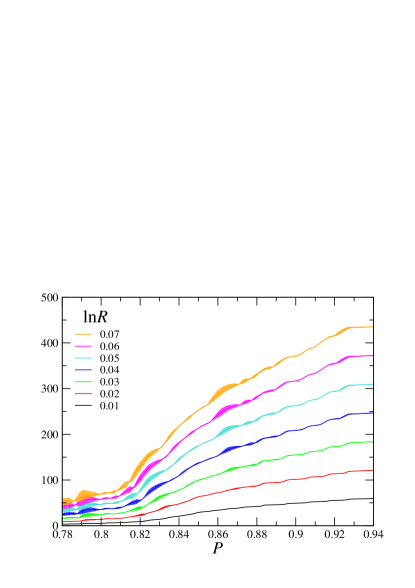
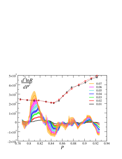
The result of is plotted in the right panel of Fig. 1. The circles with dashed lines are calculated by . The squares are computed by the numerical differential of obtained at the minimum of . are the squares in Fig. 2. It is seen that two different methods provide the consistent results.
In the calculation of , we use the delta function approximated by , where is adopted consulting the resolution and the statistical error. Because is independent of , the data obtained at various are gathered as is done in Ref. \refciteEjiri:2007ga. The results for are shown by solid curves in the left panel of Fig. 1 for – . A rapid increase is observed around . It is also important to note that the gradient becomes larger with .
The second derivative is calculated by fitting to a quadratic function of with a range of and repeating with various . The results are plotted in Fig. 1 (right), where is also shown as the circles or the squares with dashed lines. This figure shows that becomes larger with , and the maximum around exceeds for . This indicates that the curvature of the effective potential, , vanishes at and for large there exists a region of where the curvature is negative. We estimated the critical value at which the minimum of vanishes and obtained .
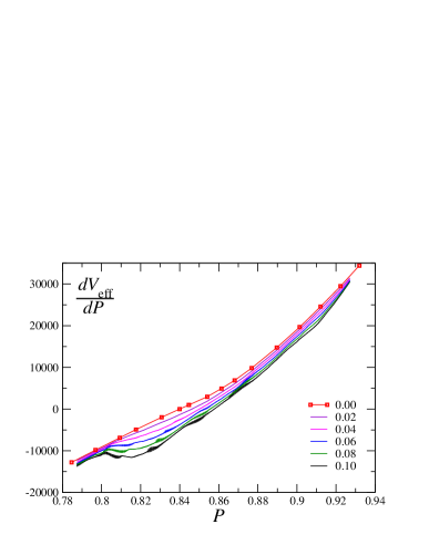
To see the appearance of the first order transition in a different way, we show at finite for in Fig. 2. The shape of the is independent of because is -independent. monotonically increases when becomes small, indicating that the transition is crossover. However, the shape of turns into an S-shape at , corresponding to the double-well potential.
 |
We defined the parameter for the Wilson quark. Then, the critical corresponding decreases as with , and the truncation error from the higher order terms in becomes smaller as increases. The application range of the hopping parameter expansion was examined in quenched QCD simulations with , by explicitly measuring the size of the next-to-leading order (NLO) terms of the expansion [18]. Then the NLO contribution turned out to be comparable to that in the leading order at . Hence, this method may be applicable up to around . For instance, in the case of with , is 0.118.
4 Conclusion and outlook
We proposed an agile method to study the thermal nature of many-flavor QCD with EWBG in TC in mind, and applied it to the 2+-flavor QCD. Fixing the mass of two light quarks, we determined the critical mass of the remaining -flavors, which separates the first order and crossover regions. The critical mass is found to become larger with . Further studies using this method are given in Ref. \refciteEjiri:2012rr, including the investigations at finite density. We find that the critical mass increases with in the 2+-flavor QCD.
The next step for the estimation of the baryon number asymmetry in TC scenario is to quantify the strength of the first order phase transition. Another interesting application of our method is to study universal scaling behavior near the tricritical point. If the chiral phase transition in the two flavor massless limit is of second order, the boundary of the first order transition region is expected to behave as in the vicinity of the tricritical point, , from the mean field analysis. This power behavior is universal for any . The density dependence is important as well, which is expected to be [19]. Starting from large , the systematic study of properties of real QCD phase transition is possible.
Acknowledgments
We would like to thank the organizers of this fruitful workshop. A part of this work was completed at GGI work shop. This work is in part supported by Grants-in-Aid of the Japanese Ministry of Education, Culture, Sports, Science and Technology (No. 22740183, 23540295 ) and by the Grant-in-Aid for Scientific Research on Innovative Areas (No. 20105002, 20105005, 23105706 ).
References
- [1] S. Weinberg, Phys. Rev. D 13, 974 (1976); L. Susskind, Phys. Rev. D 20, 2619 (1979).
- [2] B. Holdom, Phys. Rev. D 24, 1441 (1981); K. Yamawaki, M. Bando and K. i. Matumoto, Phys. Rev. Lett. 56, 1335 (1986); T. W. Appelquist, D. Karabali and L. C. R. Wijewardhana, Phys. Rev. Lett. 57, 957 (1986); T. Akiba and T. Yanagida, Phys. Lett. B 169, 432 (1986); M. Bando, T. Morozumi, H. So and K. Yamawaki, Phys. Rev. Lett. 59, 389 (1987).
- [3] L. Del Debbio, PoS (LATTICE 2010) 004 (2010); K. Rummukainen, AIP Conf. Proc. 1343, 51 (2011) and references therein.
- [4] R. D. Pisarski and F. Wilczek, Phys. Rev. D 29, 338 (1984).
- [5] S. Aoki, H. Fukaya, Y. Taniguchi and , Phys. Rev. D 86, 114512 (2012).
- [6] Z. Fodor, Nucl. Phys. Proc. Suppl. 83, 121 (2000).
- [7] For semi-quantitative analysis on electroweak baryogenesis in many flavor TC scenario, see T. Appelquist, M. Schwetz and S. B. Selipsky, Phys. Rev. D 52, 4741 (1995); Y. Kikukawa, M. Kohda and J. Yasuda, Phys. Rev. D 77, 015014 (2008).
- [8] M. E. Peskin, T. Takeuchi, Phys. Rev. Lett. 65, 964 (1990); Phys. Rev. D 46, 381 (1992).
- [9] -parameter can be calculated on the lattice. See, for example, E. Shintani et al. [JLQCD Collaboration], Phys. Rev. Lett. 101, 242001 (2008).
- [10] P. de Forcrand and O. Philipsen, Nucl. Phys. B 673, 170 (2003); JHEP 0701, 077 (2007).
- [11] Ch. Schmidt et al., Nucl. Phys. B (Proc. Suppl.) 119, 517 (2003); F. Karsch et al., Nucl. Phys. B (Proc. Suppl.) 129, 614 (2004); S. Ejiri et al., Prog. Theor. Phys. Suppl. 153, 118 (2004).
- [12] S. Ejiri et al., Phys. Rev. D 80, 094505 (2009).
- [13] S. Ejiri and N. Yamada, arXiv:1212.5899 [hep-lat], to appear in Physical Review Letter.
- [14] S. Ejiri, Phys. Rev. D 77, 014508 (2008).
- [15] H. Saito et al. (WHOT-QCD Collaboration), Phys. Rev. D 84, 054502 (2011).
- [16] C. R. Allton et al., Phys. Rev. D 71, 054508 (2005).
- [17] S. Ejiri and H. Yoneyama, PoS (LATTICE 2009) 173 (2009).
- [18] WHOT-QCD Collaboration, in preparation.
- [19] S. Ejiri, PoS (LATTICE 2008) 002 (2008).