Abstract The famous three-body problem is investigated by means of a numerical approach with negligible numerical noises in a long enough time interval, namely the Clean Numerical Simulation (CNS). From physical viewpoints, position of any bodies contains inherent micro-level uncertainty. The evaluations of such kind of inherent micro-level uncertainty are accurately simulated by means of the CNS. Our reliable, very accurate CNS results indicate that the inherent micro-level uncertainty of position of a star/planet might transfer into macroscopic randomness. Thus, the inherent micro-level uncertainty of a body might be an origin of macroscopic randomness of the universe. In addition, from physical viewpoints, orbits of some three-body systems at large time are inherently random, and thus it has no physical meanings to talk about the accurate long-term prediction of the chaotic orbits. Note that such kind of uncertainty and randomness has nothing to do with the ability of human being. All of these might enrich our knowledge and deepen our understandings about not only the three-body problem but also chaos.

Key Words Three-body problem, chaos, multiple precision, Taylor expansion, micro-level uncertainty

1 Introduction

It is well-known that the microscopic phenomena are inherent random, while many macroscopic phenomena such as moving stars and planets in the universe looks random as well. What is the origin of the macroscopic randomness? Are there any relationships between the microscopic uncertainty and the macroscopic randomness? In this article, using chaotic motion of the famous three-body problem as an example, we illustrate that the micro-level uncertainty of position of stars/planets might be one origin of the macroscopic randomness of the universe.

It is a common knowledge that some “deterministic” dynamic systems have chaotic property: their numerical simulations have sensitive dependence on initial conditions (SDIC), i.e. the so-called butterfly-effect, so that long-term accurate prediction is impossible [8, 9, 10]. Since truncation and round-off errors are unavailable for all numerical simulation techniques, nearly all numerical results given by traditional methods based on double precision are not “clean”: they are something mixd with the so-called “numerical noises”. Due to the SDIC, truncation and round-off errors enlarge exponentially so that it is very hard to gain reliable chaotic results in a long time interval. As pointed out by Lorenz [10] in 2006, different traditional numerical schemes (based on 16 or 32 digit precision) may lead to not only the uncertainty in prediction but also fundamentally different regimes of solution.

In order to gain reliable chaotic results in a long enough time interval, Liao [5] developed a numerical technique with negligible numerical noises, called the “Clean Numerical Simulation” (CNS). Using the computer algebra system Mathematica with the 400th-order Taylor expansion and data in 480-digit precision, Liao [5] obtained, for the first time, the reliable numerical results of chaotic solution of Lorenz equation in a long time interval $0\leq t\leq 1000$ Lorenz time unit (LTU). Liao’s “clean” chaotic solution of Lorenz equation was confirmed by Wang et al. [17], who employed the parallel computation and the multiple precision (MP) library to gain reliable chaotic solution up to 2500 LTU by means of the CNS approach with 1000th-order Taylor expansion and data in 2100-digit precision, and their result agrees well with Liao’s one [5] in $0\leq t\leq 1000$ LTU. This confirms the validity of the CNS approach.

It was found by Liao [5] that, to gain a reliable “clean” chaotic solution of Lorenz equation in the interval $0\leq t\leq T_{c}$, the initial conditions must be at least in the accuracy of $10^{-2T_{c}/5}$. For example, in the case of $T_{c}=1000$ LTU, the initial condition must be in 400-digit precision at least. It should be emphasized that, the 400-digit precision, which is “mathematically” necessary for the initial condition and all data at each time-step, is so high that even the statistical fluctuation of velocity and temperature becomes a very important physical factor and therefore cannot be neglected. However, from the physical viewpoints, Lorenz equation (as a macroscopical model for climate prediction on Earth) completely neglects the influence of the statistic fluctuation of velocity and temperature about the climate. Therefore, as pointed out by Liao [5], this leads to the so-called “precision paradox of chaos”.

How to avoid such kind of paradox? Traditionally, it is believed that Lorenz equation is a “deterministic” system, say, its initial condition and all physical parameters are completely certain, i.e. “absolutely accurate”. However, such kind of “absolutely accurate” variables only exist in mathematics, which have no physical meanings in practice, as mentioned below. For example, velocity and temperature of fluid are concepts defined by statistics. It is well-known that any statistical variables contain statistic fluctuation. So, strictly speaking, velocity and temperature of fluid are not “absolutely accurate” in physics. Using Lorenz equation as an example, Liao [6] pointed out that its initial conditions have fluctuations in the micro-level $10^{-30}$ so that Lorenz equation is not deterministic, from the physical viewpoint. Although $10^{-30}$ is much smaller than truncation and round-off errors of traditional numerical methods based on double precision, it is much larger than $10^{-400}$ that can be used in the CNS approach. Thus, by means of the CNS, Liao [6] accurately simulated the evaluation of the micro-level uncertainty of initial condition of Lorenz equation, and found that the micro-level uncertainty transfers into the observable randomness. Therefore, chaos might be a bridge between the micro-level uncertainty and the macroscopic randomness, as pointed out by Liao [6]. Currently, Liao [7] employed the CNS to the chaotic Hamiltonian Hénon-Heiles system for motion of stars orbiting in a plane about the galactic center, and confirmed that, due to the SDIC, the inherent micro-level uncertainty of position of stars indeed evaluates into the macroscopic randomness.

However, Lorenz equation is a greatly simplified model of Navier-Stokes equation for flows of fluid. Besides, unlike Hamiltonian Hénon-Heiles system for motion of stars orbiting in a plane, orbits of stars are three dimensional in practice. Thus, in order to further confirm the above conclusion, it is necessary to investigate some more accurate physical models, such as the famous three-body problem [3, 1, 16] governed by the Newtonian gravitation law. In fact, non-periodic results were first found by Poincaré [11] for three-body problem. In this paper, using the three-body problem as a better physical model, we employ the CNS to confirm the conclusion: the inherent micro-level uncertainty of position of a star/planet might transfer into the observable, macroscopic randomness of its orbit so that the inherent micro-level uncertainty of a star/planet might be an origin of the macroscopic randomness of the universe.

2 Approach of Clean Numerical Simulation

Let us consider the famous three-body problem, say, the motion of three celestial bodies under their mutual gravitational attraction. Let $x_{1},x_{2},x_{3}$ denote the three orthogonal axises. The position vector of the $i$ body is expressed by ${\bf r}_{i}=(x_{1,i},x_{2,i},x_{3,i})$. Let $T$ and $L$ denote the characteristic time and length scales, and $m_{i}$ the mass of the $i$th body, respectively. Using Newtonian gravitation law, the motion of the three bodies are governed by the corresponding non-dimensional equations

$$\ddot{x}_{k,i}=\sum_{j=1,j\neq i}^{3}\rho_{j}\frac{(x_{k,j}-x_{k,i})}{R_{i,j}^{3}},\;\;\;k=1,2,3,$$ (1)

where

$$R_{i,j}=\left[\sum_{k=1}^{3}(x_{k,j}-x_{k,i})^{2}\right]^{1/2}$$ (2)

and

$$\rho_{i}=\frac{m_{i}}{m_{1}},\;\;i=1,2,3$$ (3)

denotes the ratio of the mass.

In the frame of the CNS, we use the $M$-order Taylor expansion

$$x_{k,i}(t)\approx\sum_{m=0}^{M}\alpha_{m}^{k,i}\;(t-t_{0})^{m}$$ (4)

to accurately calculate the orbits of the three bodies, where the coefficient $\alpha_{m}^{k,i}$ is only dependent upon the time $t_{0}$. Note that the position $x_{k,i}(t)$ and velocity $\dot{x}_{k,i}(t)$ at $t=t_{0}$ are known, i.e.

$$\alpha_{0}^{k,i}=x_{k,i}(t_{0}),\;\;\alpha_{1}^{k,i}=\dot{x}_{k,i}(t_{0}).$$ (5)

The recursion formula of $\alpha_{m}^{k,i}$ for $m\geq 2$ is derived from (1), as described below.

Write $1/R_{i,j}^{3}$ in the Taylor expansion

$$f_{i,j}=\frac{1}{R_{i,j}^{3}}\approx\sum_{m=0}^{M}\beta_{m}^{i,j}\;(t-t_{0})^{m}$$ (6)

with the symmetry property $\beta_{m}^{i,j}=\beta_{m}^{j,i}$, where $\beta_{m}^{i,j}$ is determined later. Substituting (4) and (6) into (1) and comparing the like-power of $(t-t_{0})$, we have the recursion formula

$$\alpha_{m+2}^{k,i}=\frac{1}{(m+1)(m+2)}\sum_{j=1,j\neq i}^{3}\rho_{j}\sum_{n=0}^{m}\left(\alpha_{n}^{k,j}-\alpha_{n}^{k,i}\right)\;\beta_{m-n}^{i,j},\;\;m\geq 0.$$ (7)

Thus, the positions and velocities of the three bodies at the next time-step $t_{0}+\Delta t$ read

$$x_{k,i}(t_{0}+\Delta t) \approx \sum_{m=0}^{M}\alpha_{m}^{k,i}\;(\Delta t)^{m},$$ (8)

$$\dot{x}_{k,i}(t_{0}+\Delta t) \approx \sum_{m=1}^{M}m\;\alpha_{m}^{k,i}\;(\Delta t)^{m-1}.$$ (9)

Write

$$S_{i,j}=R^{6}_{i,j}\approx\sum_{m=0}^{M}\gamma_{m}^{i,j}\;(t-t_{0})^{m},\;\;f_{i,j}^{2}=\sum_{m=0}^{M}\sigma_{m}^{i,j}(t-t_{0})^{m},$$ (10)

with the symmetry property $\gamma_{m}^{i,j}=\gamma_{m}^{j,i}$ and $\sigma_{m}^{i,j}=\sigma^{j,i}_{m}$. Substituting (2), (4) and (6) into the above definitions and comparing the like-power of $t-t_{0}$, we have

$$\gamma^{i,j}_{m} = \sum_{n=0}^{m}\mu^{i,j}_{m-n}\sum_{k=0}^{n}\mu_{k}^{i,j}\mu_{n-k}^{i,j},$$ (11)

$$\sigma_{m}^{i,j} = \sum_{n=0}^{m}\beta^{i,j}_{n}\;\beta^{i,j}_{m-n},$$ (12)

with

$$\mu^{i,j}_{m}=\sum_{k=1}^{3}\sum_{n=0}^{m}\left(\alpha^{k,j}_{n}-\alpha^{k,i}_{n}\right)\left(\alpha^{k,j}_{m-n}-\alpha^{k,i}_{m-n}\right),\;\;i\neq j,\;m\geq 1,$$ (13)

and the symmetry $\mu_{m}^{i,j}=\mu_{m}^{j,i}$. Using the definition (6), we have

$$S_{i,j}f_{i,j}^{2}=1.$$

Substituting (10) into the above equation and comparing the like-power of $(t-t_{0})$, we have

$$\sum_{n=0}^{m}\gamma_{n}^{i,j}\;\sigma_{m-n}^{i,j}=0,\;\;m\geq 1,$$

which gives the recursion formula

$$\beta_{m}^{i,j}=-\frac{1}{2\beta_{0}^{i,j}\gamma_{0}^{i,j}}\left\{\sum_{n=1}^{m}\gamma_{n}^{i,j}\sigma_{m-n}^{i,j}+\gamma_{0}^{i,j}\sum_{k=1}^{m-1}\beta_{k}^{i,j}\beta_{m-k}^{i,j}\right\},\;\;m\geq 1,\;i\neq j.$$ (14)

In addition, it is straightforward that

$$\beta_{0}^{i,j}=\frac{1}{R_{i,j}^{3}},\;\;\;\mu_{0}^{i,j}=R_{i,j}^{2},\;\;\;\sigma_{0}^{i,j}=\left(\beta_{0}^{i,j}\right)^{2},\;\;\;\gamma^{i,j}_{0}=\left(\mu_{0}^{i,j}\right)^{3},\;\;\;\mbox{at $t=t_{0}$}.$$ (15)

It is a common knowledge that numerical methods always contain truncation and round-off errors. To decrease the round-off error, we express the positions, velocities, physical parameters and all related data in $N$-digit precision, where $N$ is a large enough positive integer. Obviously, the larger the value of $N$, the smaller the round-off error. Besides, the higher the order $M$ of Taylor expansion (4), the smaller the truncation error. Therefore, if the order $M$ of Taylor expansion (4) is high enough and all data are expressed in accuracy of long enough digits, truncation and round-off errors of the above-mentioned CNS approach (with reasonable time step $\Delta t$) can be so small that numerical noises are negligible in a given (long enough) time interval, say, we can gain “clean”, reliable chaotic numerical results with certainty in a given time interval. In this way, the orbits of the three bodies can be calculated, accurately and correctly, step by step.

In this article, the computer algebra system Mathematica is employed. By means of the Mathematica, it is rather convenient to express all datas in 300-digit precision, i.e. $N=300$. In this way, the round-off error is so small that it is almost negligible in the given time interval ($0\leq t\leq 1000$). And the accuracy of the CNS results increases as the order $M$ of Taylor expansion (4) enlarges, as shown in the next section.

3 A special example

Without loss of generality, let us consider the motion of three bodies with the initial positions

$${\bf r}_{1}=(\delta,0,-1),{\bf r}_{2}=(0,0,0),{\bf r}_{3}=-({\bf r}_{1}+{\bf r}_{2}),$$ (16)

and the initial velocities

$$\dot{\bf r}_{1}=(0,-1,0),\dot{\bf r}_{2}=(1,1,0),\dot{\bf r}_{3}=-(\dot{\bf r}_{1}+\dot{\bf r}_{2}),$$ (17)

where $\delta$ is a constant. Note that $\delta$ is the only one unknown parameter in the initial condition. For simplicity, we first only consider the three different cases: $\delta=0$, $\delta=+10^{-60}$ and $\delta=-10^{-60}$. Note that the initial velocities are the same in the three cases. Mathematically, the three initial positions have the tiny difference in the level of $10^{-60}$, which however leads to huge difference of orbits of the three bodies at $t=1000$, as shown below. For the sake of simplicity, let us consider the case of the three bodies with equal masses, i.e. $\rho_{j}=1$ ($j=1,2,3$). We are interested in the orbits of the three bodies in the time interval $0\leq t\leq 1000$.

Note that the initial conditions satisfy

$$\sum_{j=1}^{3}\dot{\bf r}_{j}(0)=\sum_{j=1}^{3}{\bf r}_{j}(0)=0.$$

Thus, due to the momentum conversation, we have

$$\sum_{j=1}^{3}\dot{\bf r}_{j}(t)=\sum_{j=1}^{3}{\bf r}_{j}(t)=0,\hskip 28.45274ptt\geq 0$$ (18)

in general.

All data are expressed in 300-digit precision, i.e. $N=300$. Thus, the round-off error is almost negligible. In addition, the higher the order $M$ of Taylor expansion (4), the smaller the truncation error, i.e. the more accurate the results at $t=1000$. Assume that, at $t=1000$, we have the result $x_{1,1}={\bf 1.81510}12345$ by means of the $M_{1}$-order Taylor expansion and the result $x_{1,1}={\bf 1.81510}47535$ by means of the $M_{2}$-order Taylor expansion, respectively, where $M_{2}>M_{1}$. Then, the result $x_{1,1}$ by means of the lower-order ($M_{1}$) Taylor expansion is said to be in the accuracy of 5 significance digit, expressed by $n_{s}=5$. For more details about the CNS, please refer to Liao [7].

Figure 1: Accuracy (expressed by $n_{s}$, number of significance digits) of the CNS results at $t=1000$ in the case of $\delta=0$ by means of $N=300$, the different time-step $\Delta t$ and the different order ($M$) of Taylor expansion. Square: $\Delta t=10^{-2}$; Circle: $\Delta t=10^{-3}$. Solid line: $n_{s}\approx 1.6762M-2.7662$; dashed line: $n_{s}\approx 2.7182M-4.2546$.

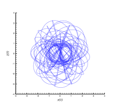
Figure 2: $x-y$ and $x-z$ of Body 1 ($0\leq t\leq 1000$) in the case of $\delta=0$.

Figure 3: $x-y$ and $x-z$ of Body 2 ($0\leq t\leq 1000$) in the case of $\delta=0$.

Figure 4: $x-y$ and $x-z$ of Body 3 ($0\leq t\leq 1000$) in the case of $\delta=0$.

When $\delta=0$, the corresponding three-body problem has chaotic orbits with the Lyapunov exponent $\lambda=0.1681$, as pointed by Sprott [13] (see Figure 6.15 on page 137). It is well-known that a chaotic dynamic system has the sensitivity dependence on initial condition ( SDIC). Thus, in order to gain reliable numerical results of the chaotic orbits in such a long interval $0\leq t\leq 1000$, we employ the CNS approach using the high-enough order $M$ of Taylor expansion with all data expressed in 300-digit precision.

It is found that, when $\delta=0$, the CNS results at $t=1000$ by means of $\Delta t=10^{-2}$, $N=300$ and $M=8,16,24,30,40$ and 50 agree each other in the accuracy of 11, 23, 38, 48, 64 and 81 significance digits, respectively. Approximately, $n_{s}$, the number of significance digits of the positions at $t=1000$, is linearly proportional to $M$ (the order of Taylor expansion), say, $n_{s}\approx 1.6762M-2.7662$, as shown in Fig. 1. For example, the CNS approach using the 50th-order Taylor expansion and data in 300-digit precision (with $\Delta t=10^{-2}$) provides us the position of Body 1 at $t=1000$ in the accuracy of 81 significance digit:

$$x_{1,1} = +1.8151047535629516172165940088454400645690$$ (19)

$$03032055743237590103285240436181354986834,$$

$$x_{2,1} = -1.4406351440582861611338350554067489001231$$ (20)

$$29002848537219768908176322703247482409938,$$

$$x_{3,1} = +1.9870078875786298810976776414985778979168$$ (21)

$$46299746397051757074.117730821734512844759.$$

Using the smaller time step $\Delta=10^{-3}$ and data in 300-digit precision (i.e. $N=300$), the CNS results given by the 8, 16, 24 and 30th-order Taylor expansion agree in the accuracy of 18, 38, 62 and 77 significance digits, respectively. Approximately, $n_{s}$, the number of significance digits of the positions at $t=1000$, is linearly proportional to $M$ (the order of Taylor expansion), say, $n_{s}\approx 2.7182M-4.2546$, as shown in Fig. 1. It should be emphasized that the CNS results by $\Delta t=10^{-3}$ and $M=30$ agree (at least) in the 77 significance digits with those by $\Delta t=10^{-2}$ and $M=50$ in the whole time interval $0\leq t\leq 1000$. In addition, the momentum conservation (18) is satisfied in the level of $10^{-295}$. All of these confirm the correction and reliableness of our CNS results. Thus, although the considered three-body problem has chaotic orbits, our numerical results given by the CNS using the 50th-order Taylor expansion and accurate data in 300-digit precision (with $\Delta t=10^{-2}$) are reliable in the accuracy of 77 significance digits in the whole interval $0\leq t\leq 1000$.

The orbits of the three bodies in the case of $\delta=0$ are as shown in Figs. 4 to 4. The orbits of Body 1 and Body 3 are chaotic. This agrees well with Sprott’s conclusion [13] (see Figure 6.15 on page 137). However, it is interesting that Body 2 oscillates along a line on the plane $z=0$. So, since $\sum_{j=1}^{3}\dot{\bf r}_{j}$ = $\sum_{j=1}^{3}{\bf r}_{j}$ = 0 due to the momentum conservation, the chaotic orbits of Body 1 and Body 3 must be symmetric about the regular orbit of Body 2. Thus, although the orbits of Body 1 and Body 3 are disorderly, the three bodies as a system have an elegant structure with symmetry.

Figure 5: Accuracy (expressed by $n_{s}$, number of significance digits) of the result at $t=1000$ in the case of $\delta=10^{-60}$ by means of $N=300$, the different time-step $\Delta t$ and the different order of Taylor expansion ($M$). Square: $\Delta t=10^{-2}$; Circle: $\Delta t=10^{-3}$. Solid line: $n_{s}\approx 0.2885M-3.4684$; dashed line: $n_{s}\approx 1.5386M-3.7472$.

Figure 6: $x-y$ and $x-z$ of Body 1 ($0\leq t\leq 1000$) in the case of $\delta=10^{-60}$.

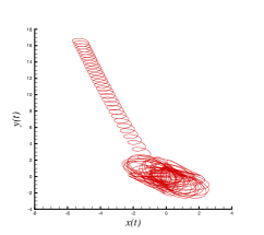
Figure 7: $x-y$ and $x-z$ of Body 2 ($0\leq t\leq 1000$) in the case of $\delta=10^{-60}$.

Figure 8: $x-y$ and $x-z$ of Body 3 ($0\leq t\leq 1000$) in the case of $\delta=10^{-60}$.

Figure 9: Orbit of Body 1 ($0\leq t\leq 1000$). Left: $\delta=0$; Right: $\delta=10^{-60}$.

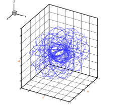
Figure 10: Orbit of Body 2 ($0\leq t\leq 1000$). Left: $\delta=0$; Right: $\delta=10^{-60}$.

Figure 11: Orbit of Body 3 ($0\leq t\leq 1000$). Left: $\delta=0$; Right: $\delta=10^{-60}$.

The initial conditions when $\delta=10^{-60}$ have a tiny difference

$$d{\bf r}_{1}=10^{-60}(1,0,0)$$

from those when $\delta=0$. Thus, it is reasonable to assume that the corresponding dynamic system is chaotic, too. Similarly, the corresponding orbits of the three bodies can be accurately simulated by means of the CNS. It is found that, when $\delta=10^{-60}$, the CNS results at $t=1000$ by means of $\Delta t=10^{-2}$, $N=300$ and $M$ = 16, 24, 30, 40, 50, 60 , 70, 80, 100 agree each other in the accuracy of 1, 3, 5, 9, 11, 14, 17, 19 and 27 significance digits, respectively. Approximately, $n_{s}$ (the number of significance digits) is linearly proportional to $M$ (the order of Taylor expansion), say, $n_{s}\approx 0.2885M-3.4684$, as shown in Fig. 5. According to this formula, in order to have the CNS results (at $t=1000$) in the precision of 81 significance digits by means of $\Delta t=10^{-2}$, the 300th-order of Taylor expansion, i.e. $M=300$, must be used. But, this needs much more CPU time. To confirm the correction of these CNS results, we further use the smaller time step $\Delta t=10^{-3}$. It is found that, when $\delta=10^{-60}$ , the results at $t=1000$ by means of the CNS using $\Delta t=10^{-3}$, $N=300$ and $M$ = 8, 16, 24, 30, 40, 50 agree well in the precision of 8, 21, 33, 43, 59, 72 significance digits, respectively. Approximately, $n_{s}$, the number of significance digits of the corresponding results at $t=1000$, is linearly proportional to $M$ (the order of Taylor expansion), say, $n_{s}\approx 1.5386M-3.7472$, as shown in Fig. 5. For example, the position of Body 1 at $t=1000$ given by the 50th-order Taylor expansion and data in 300-digit precision with $\Delta t=10^{-3}$ reads

$$x_{1,1} = +10.5718991771626848605399651180233387355185816$$ (22)

$$19035776331820966524368101464,$$

$$x_{2,1} = -33.3956860196582147031781512361768602407559680$$ (23)

$$29199276186710038142873929480,$$

$$x_{3,1} = +20.2845527396821922952136869217938844104404153$$ (24)

$$94341528671055848805097262214,$$

which are in the precision of 72 significance digits. Note that the positions of the three bodies at $t=1000$ given by $\Delta t=10^{-2}$ and $M=100$ agree well (in precision of 27 significance digits) with those by $\Delta t=10^{-3}$ and $M=50$. In addition, the momentum conservation (18) is satisfied in the level of $10^{-293}$. Thus, our CNS results in the case of $\delta=10^{-60}$ are reliable in the interval $0\leq t\leq 1000$ as well.

The orbits of the three bodies in the case of $\delta=10^{-60}$ are as shown in Figs. 8 to 8. It is found that, in the time interval $0\leq t\leq 800$, the orbits of the three bodies are not obviously different from those in the case of $\delta=0$, say, Body 2 oscillates along the same line on $z=0$, Body 1 and Body 3 are chaotic with the same symmetry about the regular orbit of Body 2. However, the obvious difference of orbits appears when $t\geq 810$: Body 2 departs from the oscillations along the line on $z=0$ and escapes (together with Body 3) along a complicated three-dimensional orbit. Besides, Body 1 and Body 3 escape in the opposite direction without any symmetry. As shown in Figs. 11 to 11, Body 2 and Body 3 go far and far away from Body 1 and thus become a binary-body system. Thus, it is very interesting that, the tiny difference $d{\bf r}_{1}=10^{-60}(1,0,0)$ of the initial conditions finally disrupts not only the elegant symmetry of the orbits but also even the three-body system itself!

Figure 12: Orbit of Body 1 ($0\leq t\leq 1000$). Left: $\delta=+10^{-60}$; Right: $\delta=-10^{-60}$.

Figure 13: Orbit of Body 2 ($0\leq t\leq 1000$). Left: $\delta=+10^{-60}$; Right: $\delta=-10^{-60}$.

Figure 14: Orbit of Body 3 ($0\leq t\leq 1000$). Left: $\delta=+10^{-60}$; Right: $\delta=-10^{-60}$.

Similarly, in the case of $\delta=-10^{-60}$, we gain the reliable orbits of the three bodies by means of the CNS with $\Delta t=10^{-3}$, $N=300$ and $M=20$ (i.e. the 20th-order Taylor expansion). As shown in Figs. 14 to 14, the tiny difference in the initial position disrupts not only the elegant symmetry of the orbits but also the three-body system itself as well: when $t>810$, Body 2 departs from its oscillation along the line on $z=0$ and escapes (but together with Body 1) in a complicated three-dimensional orbit, while Body 1 and Body 3 escape in the opposite direction without any symmetry. Note that, in the case of $\delta=-10^{-60}$, Body 1 and Body 2 go together far and far away from Body 3 to become a binary system. However, in the case of $\delta=+10^{-60}$, Body 2 and Body 3 escape together to become a binary system! This is very interesting. Thus, the orbits of the three-body system when $\delta=0$, $\delta=+10^{-60}$ and $\delta=-10^{-60}$ are completely different.

From the mathematical viewpoints, the above results are not surprising at all and thus there exist nothing new: since the three-body system is chaotic (as pointed out by Sprott [13]), the results are certainly very sensitive to the initial conditions. However, the difference of the three initial positions is so small that they can be regarded as the same in physics! In other words, from physical viewpoints, such a small difference in space has no physical meanings at all, and thus the three initial conditions (when $\delta=0$ and $\delta=\pm 10^{-60}$, respectively) are the same in physics. This is mainly because position of any a body inherently contains the micro-level uncertainty so that the three-body system is not deterministic, as explained below.

It is well known that the microscopic phenomenon are essentially uncertain/random. Let us first consider some typical length scales of microscopic phenomenon which are widely used in modern physics. For example, Bohr radius

$$r=\frac{\hbar^{2}}{m_{e}\;e^{2}}\approx 5.2917720859(36)\times 10^{-11}\;\;\mbox{(m)}$$

is the approximate size of a hydrogen atom, where $\hbar$ is a reduced Planck’s constant, $m_{e}$ is the electron mass, and $e$ is the elementary charge, respectively. Besides, the so-called Planck length

$$l_{P}=\sqrt{\frac{\hbar\;G}{c^{3}}}\approx 1.616252(81)\times 10^{-35}\;\;\;\mbox{(m)}$$ (25)

is the length scale at which quantum mechanics, gravity and relativity all interact very strongly, where $c$ is the speed of light in a vacuum and $G$ is the gravitational constant. According to the string theory [12], the Planck length is the order of magnitude of oscillating strings that form elementary particles, and shorter length do not make physical senses. Especially, in some forms of quantum gravity, it becomes impossible to determine the difference between two locations less than one Planck length apart. Therefore, in the level of the Planck length, position of a body is inherently uncertain. This kind of microscopic physical uncertainty is inherent and has nothing to do with Heisenberg uncertainty principle [4] and the ability of human being as well.

In addition, according to de Broglie [2], any a body has the so-called wave-particle duality. The de Broglie’s wave of a body has non-zero amplitude. Thus, position of a body is uncertain: it could be almost anywhere along de Broglie’s wave packet. Thus, according to the de Broglie’s wave-particle duality, position of a star/planet is inherent uncertain, too. Therefore, it is reasonable to assume that, from the physical viewpoint, the micro-level inherent fluctuation of position of a body shorter than the Planck length $l_{p}$ is essentially uncertain and/or random.

To make the Planck length $l_{p}\approx 1.62\times 10^{-35}$ (m) dimensionless, we use the dimeter of Milky Way Galaxy as the characteristic length, say, $d_{M}\approx 10^{5}$ light year $\approx 9\times 10^{20}$ meter. Obviously, $l_{p}/d_{M}\approx 1.8\times 10^{-56}$ is a rather small dimensionless number. Thus, as mentioned above, two (dimensionless) positions shorter than $10^{-56}$ do not make physical senses in many cases. So, it is reasonable to assume that the inherent uncertainty of the dimensionless position of a star/planet is in the micro-level $10^{-60}$. Therefore, the tiny difference $d{\bf r}_{1}=\pm 10^{-60}(1,0,0)$ of the initial conditions is in the micro-level: the difference is so small that all of these initial conditions can be regarded as the same in physics!

Mathematically, $10^{-60}$ is a tiny number, which is much smaller than truncation and round-off errors of traditional numerical approaches based on data of 16-digit precision. So, it is impossible to investigate the influence and evaluation of this inherent micro-level uncertainty of initial conditions by means of the traditional numerical approaches. However, the micro-level uncertainty $10^{-60}$ is much larger than the truncation and round-off errors of the CNS results gained by means of the high-order Taylor expansion and data in 300-digit precision with a reasonable time step $\Delta t$, as illustrated above. So, the CNS provides us a convenient tool to study the transfer and evaluation of such kind of inherent micro-level uncertainty of initial conditions.

The key point is that such an inherent micro-level uncertainty in the initial conditions finally leads to the huge, observable difference of orbits of the three bodies: it disrupts not only the elegant symmetry of the orbits but also the three-body system itself. Note that, Body 2 escapes with Body 3 in the case of $\delta=+10^{-60}$, but with Body 1 in the case of $\delta=-10^{-60}$, to become a binary-body system! In nature, such kind of inherent micro-level uncertainty exists for each body at any time $t\geq 0$. So, from the physical viewpoint, the orbits of each body at large enough time are inherently unknown, i.e. random: given the same initial condition (in the viewpoint of physics), the orbits of the three-body system under consideration might be completely different. For example, the three-body system might either have the elegant symmetry, or disrupt as the different binary-body systems, as shown in Figs. 11 to 11, and Figs. 14 to 14, respectively.

Note that, from mathematical viewpoint, we can accurately simulate the orbits of three bodies in the interval $0\leq t\leq 1000$. However, due to the inherent position uncertainty and the SDIC of chaos, orbits of the three bodies are random when $t>810$, since the inherent position uncertainty transfers into macroscopic randomness. Thus, from physical viewpoint, there exists the maximum predictable time $T^{p}_{max}$, beyond which the orbits of the three bodies are inherently random and thus can not be predictable in essence. Note that $T^{p}_{max}$ is determined by the inherent position uncertainty of the three bodies, which has nothing to do with the ability of human being. Therefore, long term “prediction” of chaotic dynamic system of the three bodies is mathematically possible, but has no physical meanings!

Finally, to confirm our above conclusions, we further consider such a special case with the micro-level uncertainty of the initial position $d{\bf r}_{1}=10^{-60}(1,1,1)$, i.e.

$${\bf r}_{1}=(0,0,-1)+10^{-60}(1,1,1).$$

It is so tiny that, from the physical viewpoint mentioned above, the initial positions can be regarded as the same as those of the above-mentioned three cases. However, the corresponding orbits of the three bodies (in the time interval $0\leq t\leq 1200$) obtained by means of the CNS with $\Delta t=10^{-3},N=300$ and the 30th-order Taylor expansion ($M=30$) are quite different from those of the three cases: Body 2 first oscillates along a line on $z=0$ but departs from the regular orbit for large $t$ to move along a complicated three-dimensional orbits, while Body 1 and Body 3 first move with the symmetry but lose it for large $t$, as shown in Figs. 17 to 17. However, it is not clear whether any one of them might escape or not, i.e. the fate of the three-body system is unknown. Since such kind of micro-level uncertainty of position is inherent and unknown, given the same (from the physical viewpoint) initial positions of the three bodies, the orbits of the three-body system at large enough time is completely unknown. So, it has no physical meanings to talk about the accurate long-term prediction of orbits of the three-body system, because the orbits at large time (such as $t\geq 1000$) is inherently unknown/random and thus should be described by probability. This is quite similar to the motion of electron in an atom. It should be emphasized that, such kind of transfer from the inherent micro-level uncertainty to macroscopic randomness is essentially due to the SDIC of chaos, but has nothing to do with the ability of human being and Heisenberg uncertainty principle [4].

Figure 15: Orbit of Body 1 ($0\leq t\leq 1200$) when $d{\bf r}_{1}=10^{-60}\;\;(1,1,1)$.

Figure 16: Orbit of Body 2 ($0\leq t\leq 1200$) when $d{\bf r}_{1}=10^{-60}\;\;(1,1,1)$.

Figure 17: Orbit of Body 3 ($0\leq t\leq 1200$) when $d{\bf r}_{1}=10^{-60}\;\;(1,1,1)$.

All of these reliable CNS results indicate that, due to the SDIC of chaos, such kind of inherent micro-level uncertainty of a star/planet might transfer into macroscopic randomness. This provides us an explanation for the macroscopic randomness of the universe, say, the inherent micro-level uncertainty might be an origin of the microscopic randomness, although it might be not the unique one. This might enrich and deepen our understandings about not only the three-body problem but also the chaos.

4 Conclusions

The famous three-body problem is investigated by means of a numerical approach with negligible numerical noises in a long enough time interval, namely the Clean Numerical Simulation (CNS). From physical viewpoints, position of any bodies contains inherent micro-level uncertainty. The evaluations of such kind of inherent micro-level uncertainty are accurately simulated by means of the CNS. Our reliable, very accurate CNS results indicate that the inherent micro-level uncertainty of position of a star/planet might transfer into macroscopic randomness. Thus, the inherent micro-level uncertainty of a body might be an origin of macroscopic randomness of the universe. In addition, from physical viewpoints, orbits of some three-body systems at large time are inherently random, and thus it has no physical meanings to talk about the accurate long-term prediction of the chaotic orbits. Note that such kind of uncertainty and randomness has nothing to do with the ability of human being and Heisenberg uncertainty principle [4].

In this article, we introduce a new concept: the maximum predictable time $T^{p}_{max}$ of chaotic dynamic systems with physical meanings. For the chaotic motions of the three body problem considered in this article, there exists the so-called maximum predictable time $T^{p}_{max}\approx 810$, beyond which the motion of three bodies is sensitive to the micro-level inherent uncertainty of position and thus becomes inherently random in physics. The so-called maximum predictable time of chaotic three bodies is determined by the inherent uncertainty of position and has nothing to do with the ability of human being. Note that, from the mathematically viewpoint, we can accurately calculate the orbits by means of the CNS in the interval $0\leq t\leq 1000$. Thus, considering the physical inherent uncertainty of position, long term “prediction” of chaotic motion of the three bodies is mathematically possible but has no physical meanings.

In summary, our rather accurate computations based on the CNS about the famous three-body problem illustrate that, the inherent micro-level uncertainty of positions of starts/planets might be one origin of macroscopic randomness of the universe. This might enrich our knowledge and deepen our understandings about not only the three-body problem but also chaos. Indeed, the reliable computations based on the CNS are helpful for us to understand the world better.

Note that the computation ability of human being plays an important role in the development of chaotic dynamic systems. The finding of SDIC of chaos by Lorenz in 1963 is impossible without digit computer, although data used by Lorenz in his pioneering work is only in accuracy of 16-digits precision. So, the CNS with negligible numerical noises provides us a useful tool to understand chaos better.

Finally, as reported by Sussman and Jack [14, 15], the motion of Pluto and even the solar system is chaotic with a time scale in the range of 3 to 30 million years. Thus, due to the SDIC of chaos and the micro-level inherent uncertainty of positions of planets, the solar system is in essence random. Note that such kind of randomness has nothing to do with the ability of human: the history of human being is indeed too short, compared to the time scale of such kind of macroscopic randomness. The determinism is only a concept of human being: considering the much shorter time-scale of the human being, one can still regard the solar system to be deterministic, even although it is random in essence.

References

- [1] Diacu, F. and Holmes, P.: Celestial Encounters: The Origins of Chaos and Stability. Princeton University Press, Princeton , 1996.
- [2] de Broglie, L.: Recherches sur la thèorie des quanta (Researches on the quantum theory), Thesis, Paris, 1924.
- [3] Hénon, M. and Heiles, C.: The applicability of the third integral of motion: some numerical experiments. Astrophys. J., 69:73 – 79, 1964.
- [4] Heisenberg, W.: Über den anschaulichen Inhalt der quantentheoretischen Kinematik und Mechanik, Zeitschrift für Physik, 43 (3-4): 172 –198, 1927.
- [5] Liao, S.J.: On the reliability of computed chaotic solutions of non-linear differential equations. Tellus-A, 61: 550 – 564, 2009. (arXiv:0901:2986)
- [6] Liao, S.J.: Chaos – a bridge from micro-level uncertainty to macroscopic randomness. Communications in Nonlinear Science and Numerical Simulation. 17: 2564-2569, 2012. (arXiv:1108.4472)
- [7] Liao, S.J.: On the numerical simulation of propagation of micro-level uncertainty for chaotic dynamic systems. Chaos, Solitons and Fractals, accepted (arXiv:1109.0130).
- [8] Lorenz, E.N.: Deterministic non-periodic flow. Journal of the Atmospheric Sciences, 20: 130 – 141, 1963.
- [9] Lorenz, E.N.: The essence of Chaos. University of Washington Press, Seattle, 1993.
- [10] Lorenz, E.N.: Computational periodicity as observed in a simple system. Tellus-A, 58: 549 – 59, 2006.
- [11] Poincaré, J.H.: Sur le problème des trois corps et les équations de la dynamique. Divergence des séries de M. Lindstedt. Acta Mathematica, 13:1 – 270, 1890.
- [12] Polchinski, J.: String Theory. Cambridge University Press, Cambridge, 1998.
- [13] Sprott, J.C.: Elegant Chaos. World Scientific, New Jersey, 2010.
- [14] Sussman, G.J. and Jack, J.: Numerical Evidence that the Motion of Pluto is Chaotic. Science, 241: 433 – 437, 1988.
- [15] Sussman, G.J. and Jack, J.: Chaotic Evolution of the Solar System. Science, 257: 56 – 62, 1992.
- [16] Valtonen, M. and Karttunen, H.: The three-body problem. Cambridge University, Cambridge, 2005.
- [17] Wang, P.F., Li, J.P. and Li, Q.: Computational uncertainty and the application of a high-performance multiple precision scheme to obtaining the correct reference solution of Lorenz equations. Numerical Algorithms, 59: 147 – 159, 2012.