A Stochastic Delay Model for Pricing Debt and Equity: Numerical Techniques and Applications.

Abstract

In the accompanied paper [14], a delayed nonlinear model for pricing corporate liabilities was developed. Using self-financed strategy and duplication we were able to derive two Random Partial Differential Equations (RPDEs) describing the evolution of debt and equity values of the corporate in the last delay period interval. In this paper, we provide numerical techniques to solve our delayed nonlinear model along with the corresponding RPDEs modeling the debt and equity values of the corporate.

Using financial data from some firms, we compare numerical solutions from both our nonlinear model and classical Merton model [7] to the real corporate data. From this comparison, it comes up that in corporate finance the past dependence of the firm value process may be an important feature and therefore should not be ignored.

1 Introduction

Due to the remarkable growth of the credit derivatives market, the interest in corporate claim value models and risk structure has recently increased. Financial distress tends to be an important factor in many corporate decisions. The two main sources of financial distress are corporate illiquidity and insolvency. In his paper [2], Gryglewicz explains how changes in solvency affect liquidity and also how liquidity concerns affect solvency via capital structure choice. Corporate solvency is the ability to cover debt obligations in the long run. Uncertainty about average future profitability, with financial leverage, generates solvency concerns. Corporate insolvency may lead to corporate reorganization or to bankruptcy of the firm in the worst case. Corporate bankruptcy is central to the theory of the firm. A firm is generally considered bankrupt when it cannot meet a current payment on a debt obligation. In this event, the equity holders lose all claims on the firm, and the remaining loss which is the difference between the face value of the fixed claims and the market value of the firm, is supported by the debt holders. In the literature of corporate finance, Merton [7] appears to be the main pioneers in the derivation of formulas for corporate claims. This model is a dual of Black and Scholes model [12] for stock price. Merton [7] further analyzed the risk structure of interest rates. More specifically, he found the relation between corporate bond spreads and government bond, and attempted to determine a valid measure of risk. He also developed the deterministc partial differential equation modelling the debt and equity of the firm. The assumption of constant volatility in the original Black-Scholes and Merton models from which most claims derivations are inspired, is incompatible with derivatives prices observed in the market (see [3, 4, 6, 5] and the references therein). For stock price, two alternative theories are mostly used to overcome the constant volatility drawback. The first approach sometime called level-dependent volatility describes the stock price as a diffusion with level dependent volatility [10]. The second approach sometime called stochastic volatility defines the volatility as an autonomous diffusion driven by a second Brownian motion.

In [17], a new class of nonconstant volatility model which can be extended to include the first of the above approaches, that we called delayed model is introduced and further study in [9, 16] for options prices. This model shows that the past dependence of the stock price process is an important feature and therefore should not be ignored. The main goal of this model is to make volatility self–reinforcing. Since the volatility is defined in terms of past behavior of the asset price, the self–reinforcing is high, precisely when there have been large movements in the recent past (see [17]). This is designed to reflect real–world perceptions of market volatility, particularly if practitioners are to compare historic volatility with implied.

Following the duality between the stock price [12] and corporate finance [7], we have recently introduced in [13, 14] the nonlinear delayed model in debt and guarantee. Using self-financed strategy and replication we established that debt value and equity value follow two similar Random Partial differential Equations (RPDEs) within the last delay period interval . The analytical solution of our nonlinear model and RPDEs are unknown in general case and therefore numerical techniques are needed.

In recent years, the computational complexity of mathematical models employed in financial mathematics has witnessed a tremendous growth (see [22, 21, 15] and references therein). The aims of this paper is to solve numerically our delayed nonlinear model for firm market value along with the corresponding RPDEs, using real data from firms. Comparison will be done with classical Merton model. To the best of our knowledge such comparison has not yet been done in the financial literature. Two major comparisons will be preformed: the market value of each corporate and its equity value (or its debt value). We will first approximate the volatility of each corporate, afterward solve numerically our nonlinear model for the market value of the corporate along with the corresponding Merton model using the $\theta-$ semi implicit Euler Maruyama scheme to obtain sample numerical solutions. Monte carlo method will be thereafter used to approximate the mean numerical solution of each model. The meam numerical value from each model (our nonlinear model and Merton model) will be therefore compared with the real market value ($V$) of the corporate. For debt value (or equity value) solutions of RPDEs established in the accompanied paper [14], efficient numerical scheme based on finite volume-finite difference methods (discretization respect to the firm value $V$) and exponential integrator (discretization respect to the time $t$) will be used. Recently, exponential integrators have been used efficiency in many applications in porous media flow [1, 20, 19, 25, 26], but are not yet well spread in finance. The same numerical technique is also used to solve deterministic Partial Differential Equations (PDEs) modeling debt value or equity value in Merton model. Comparisons are done with the real data from firms for each model (our delay model and Merton model).

From our comparison, it comes up that in corporate finance the past dependence of the firm value process is an important feature and therefore should not be ignored. The main goal of this paper is to call for further attention into the possibility of modeling market value of the firm with nonlinear delayed stochastic differential equations.

The paper is organized as follows. In Section 4, we recall our delayed nonlinear model for corporate claims as presented in [14] along with the Merton model [7]. In Section 3, numerical techniques for our delayed nonlinear model are provided. We first present the $\theta-$ semi implicit Euler Maruyama for the firm market value $V$ and provide numerical experimentations for both our nonlinear model and Merton model using real data for some firms. We end this section by providing numerical technique to solve efficiently our (RPDEs) modeling the debt and equity of the firm along with numerical experimentations for the two models (our delayed nonlinear model and Merton model) with real data for some firms. The conclusion is provided in Section 4.

2 Stochastic delay model for corporate claims

Here we present the stochastic delay model formulated in the accompanied paper [14] along with Random Partial Differential Equation (RPDE) that should satisfy any claim. We assume that:

• The value of the company is unaffected by how it is financed (the capital structure irrelevance principle).

• The market value of firm at time $t\in[0,T]$, $V(t)$, follows a nonlinear Stochastic Delay Differential Equation (SDDE)

  $$\left\{\begin{array}[]{l}dV(t)=(\alpha V(t)V(t-L)-C)dt+g(V(t-L))V(t)dW(t)\\ \newline \\ V(t)=\varphi(t),\,\,t\in[-L,0]\\ \end{array}\right.$$ (4)

  on a probability space $(\Omega,\mathcal{F},P))$ with a filtration $(\mathcal{F}_{0\leq t\leq T})$ satisfying the usual conditions.

where $\alpha$ is the riskless interest rate of return on the firm per unit time, $C$ is the total amount payout by the firm per unit time to either the shareholders or claims-holders (e.g. dividends or interest payments) if positive, and it is the net amount received by the firm from new financing if negative. The constant $L$ represents the past length while $T$ is the maturity date. The function $g:\mathbb{R}\rightarrow\mathbb{R}$ is a continuous representing the volatility function on the firm value per unit time. The initial process $\varphi:\Omega\rightarrow C([-L,0],\mathbb{R})$ is $\mathcal{F}_{0}$-measurable with respect to the Borel $\sigma$-algebra of $C([-L,0],\mathbb{R})$, actually $\varphi$ is the past value of the firm. The process $W$ is a one dimensional standard Brownian motion adapted to the filtration $(\mathcal{F}_{t})_{0\leq t\leq T}$.

Notice that $C$ and $\alpha$ can be time dependent functions, in which case they should be measurable and integrable in the interval $[0,T]$.

The results ensuring the feasiblility of the price model (4) is given in [7, 13]. Following the work in [7], in order the RPDE which must be satisfied by any security whose value can be written as a function of the value of the firm and time, we assume that any claim with market value $Y(t)$ (which can be replicated using self-financed strategy) at time $t$ with $Y(t)=F(V(t),t)$ follows a nonlinear stochastic delay differential equation

$$\left\{\begin{array}[]{l}dY(t)=(\alpha_{y}Y(t)-C_{y})dt+g_{y}(Y(t-L))Y(t)dW_{y}(t),\,\,t\in[0,T]\\ \newline \\ Y(t)=\varphi_{y}(t),\,\,t\in[-L,0],\end{array}\right.$$ (8)

on a probability space $(\Omega,\mathcal{F},P))$. where $\alpha_{y}$ is the constant riskless interest rate of return per unit time on this claim; $C_{y}$ is the amount payout per unit time to this claim; $g_{y}:\mathbb{R}\rightarrow\mathbb{R}$ is a continuous function representing the volatility function of the return on this claim per unit time; the initial process $\varphi_{y}:\Omega\rightarrow C([-L,0],\mathbb{R})$ is $\mathcal{F}_{0}$-measurable with respect to the Borel $\sigma$-algebra of $C([-L,0],\mathbb{R})$. The functions $C_{y}(t)$ and $\alpha_{y}(t)$ are measurable and integrable in the interval $[0,T]$. The process $W_{y}$ is a one dimensional standard Brownian motion adapted to the filtration $(\mathcal{F}_{t})_{0\leq t\leq T}$. For any claim $Y(t)=F(V(t),t)$ where $F$ is twice continuously differentiable with respect to $V$ and once differentiable with respect to $t$, we have proved in [14] that the following (RPDE) should be satisfied

$$\dfrac{1}{2}g^{2}(V(t-L))v^{2}F_{vv}+(rv-C)F_{v}+F_{t}-rF+C_{y}=0,$$ (9)

$$\qquad\qquad\,(t,v)\in[T-L,T]\times\mathbb{R}^{+}$$ (10)

with

$$F_{t}(v,t)=\frac{\partial F(v,t)}{\partial t},\,F_{v}(v,t)=\frac{\partial F(v,t)}{\partial v},\,F_{vv}(v,t)=\frac{\partial^{2}F(v,t)}{\partial v^{2}}.$$

By setting

$$V(t)=F(V(t),t)+f(V(t),t),$$ (11)

where $f(V(t),t)$ is the value of the equity, $F(V(t),t)$ the value of debt a any time $t$ before the maturity and $r$ is the instantaneous riskless rate of interest. We have obtained in [14] the following two final value problems for debt and equity, linked by (11)

$$\left\{\begin{array}[]{l}\dfrac{1}{2}g^{2}(V(t-L))v^{2}F_{vv}+(rv-C)F_{v}+F_{t}-rF+C_{y}=0,\,\,t\in(T-L,T)\\ \newline \\ F(v,T)=\min[V,B],\,\,\,\,v>0\\ \newline \\ F(0,t)=0,\,\,\,\,F(v,t)\sim Be^{-r(T-t)},\text{ as }v\rightarrow\infty,\end{array}\right.$$ (17)

and

$$\left\{\begin{array}[]{l}\dfrac{1}{2}g^{2}(V(t-L))v^{2}f_{vv}+(rv-C)f_{v}-rf+C-C_{y}+f_{t}=0,\,\,t\in(T-L,T)\\ \newline \\ f(v,T)=\max(v-B,0),\,\,\,\,\,v>0\\ \newline \\ f(0,t)=0,\,\,\,\,f(v,t)\sim v-Be^{-r(T-t)},\text{ as }v\rightarrow\infty,\end{array}\right.$$ (23)

where $B$ is the promised value the firm must pay to the debtholders at the maturity date $T$.

Remark 2.1.

The classical Merton model [7] assumes that the value of the firm at time $t\in[0,T]$, $V(t)$, follows a Stochastic Differential Equation (SDE)

$$\left\{\begin{array}[]{l}dV=(\alpha V-C)dt+\sigma VdW\\ \newline \\ V(0)\,\,\text{given},\\ \end{array}\right.$$ (27)

where $\sigma^{2}$ is the constant instantaneous variance of the return on the firm per unit time. In this case, the equity value $f$ should satisfy the following deterministc PDE

$$\left\{\begin{array}[]{l}\dfrac{1}{2}\sigma^{2}v^{2}f_{vv}+(rv-C)f_{v}-rf+C-C_{y}+f_{t}=0,\,\,t\in(0,T)\\ \newline \\ f(v,T)=\max(v-B,0),\,\,\,\,\,v>0\\ \newline \\ f(0,t)=0,\,\,\,\,f(v,t)\sim v-Be^{-r(T-t)},\text{ as }v\rightarrow\infty.\end{array}\right.$$ (33)

3 Numerical techniques and applications

3.1 Presentation of the data set and volatility estimation

The data on stock returns come from the Center for Research in Securty Prices(CRSP) database: http://www.crsp.com/ while those on debt values are from the Research Insight/Compustat database (http://www.compustat.com/). More data include firms that had valid data for all 20 years from 1991-2010 and including:

1. The risk free rate $r$ per year, which is the average monthly yield on US T-Bills for that year (the same for all firms each year).

2. The standard deviation of daily returns $\sigma$ per year for each firm.

3. The number of daily returns $N$ used to compute $\sigma$ for each firm each year (this is set to be at least 150).

4. The total book value of debt $B$ (in 1,000,000’s).

5. The total value of the firm’s assets $V$ (in 1,000,000’s).

6. The total amount $C$ (in 1,000,000’s) payout by the firm per unit time to either the shareholders or claims-holders for 10 years (2000-2010).

7. The total amount $C_{y}$ (in 1,000,000’s) payout per unit time for the debt within 10 years (2000-2010).

In fact the data set we have used include all the parameters that we need to solve either the stochastic differential equations (4) & (27), or the RPDE (17) & (23) and the PDE (33).

All the simulation is performed in Matlab 7.7. In most of our simulations, the data between 1991-2000.5 are used as memory data while those between 2000.5-2010 are used as the future data i.e. the data that we want our model to predict.

To estimate the volatility function $g$, we use the quadratic or linear interpolation of the memory part of data $\sigma$. As in [3], the quadratic form of the volatility is motivated by the fact that the implied volatility in Black-Scholes model has a parabolic shape. The volatility function $g$ can also be estimateed by using the splines interpolation of the memory part of the data $\sigma$.

As we only have yearly data set, we use also the interpolation to have more data set if need as the numerical schemes usually need small time step (then more data set) to ensure their stabilities.

3.2 Numerical approximation of the corporate market value

3.2.1 The $\theta-$ semi implicit Euler-Maruyama scheme

Here we consider the stochastic equations (4) and (27) within the time interval $[0,T]$, where the higher value of $T$ is 9.5 corresponding to the year $2010$. The time unit being the year. Indeed the values of $\alpha$ and $C$ are time depending, we therefore consider those values as two time depending functions, which are constant within each year interval. The goal here is to use the mean numerical solutions of the firm $V$ as the forecasting values of firm in the interval $[2000.5,2000.5+T]$. As the real firm value of the companies are already known in that interval, the aim is to see how close are the forecasting firm values (from numerical methods) comparing to the real firm values from financial industries. Recall that our nonlinear model used the memory data within the interval $[1991,2000.5]$. We solve numerically our nonlinear model (4) for the value of the company and Merton model (27) in time using the $\theta-$ implicit Euler Maruyama scheme in order to obtain numerical sample solutions. Monte carlo method is thereafter used to approximate the mean numerical solution of each model. The mean numerical value from each model will be therefore compared with the real company value $V$.

The $\theta-$ semi implicit Euler-Maruyama scheme applied to (4) is given by

$$V_{n+1} = V_{n}+\Delta T\left[\theta(\alpha_{n+1}V_{n+1}V_{n-m+1}-C_{n+1})+(1-\theta)(\alpha_{n}V_{n}V_{n-m}-C_{n})\right]$$ (34)

$$\;\;+g(V_{n-m})V_{n}\Delta W_{n}\;\;\;\;n=1.......,M,\;\;0\leq\theta\leq 1,\;\;\;L=m\Delta T.$$

where $\Delta T=T/M$ is the time step size, $M$ the total number of time subdivision, $V_{n}$ is the approximation of $V(t_{n}),\,t_{n}=n\Delta T$, $\alpha_{n}=\alpha(t_{n})$, $C_{n}=C(t_{n})$, and

$$\Delta W_{n}=W(t_{n+1})-W(t_{n})$$

are standard Brownian increments, independent identically distributed
$\sqrt{\Delta T}\mathcal{N}(0,1)$ random variables. For $\theta=0$, we have the classical Euler-Maruyama scheme which is less numerical stable than the semi implicit Euler-Maruyama with $\theta=1$, that we will use in our simulation. To ensure the convergence of the numerical (34) toward the unique solution of (4), the volatility function $g$ need to be globally Lipschitz, or localy Lipschitz and bounded [16]. These conditions are sufficient conditions for the convergence and not necessary conditions since the scheme can converge for some functions not verifying these conditions.

To approximate the expected value (mean) of the process $V$, we use the Monte Carlo method to compute the mean of the numerical samples from (34). The Monte Carlo method can also be used to approximate any moment of the process $V$.

3.2.2 Application with corporate data

The following firms are used:

• Great Northern Iron Ore Pptys (Figure 3 and Figure 3)

• Tor Minerals Intl Inc (Figure 3 and Figure 3)

• South Jersey Inds Inc (Figure 2 and Figure 2)

• Rentech Inc (Figure 1 and Figure 1)

• Magna International Inc (Figure 1 and Figure 1)

• First Citizens Bancshares Inc NC (Figure 2 and Figure 2)

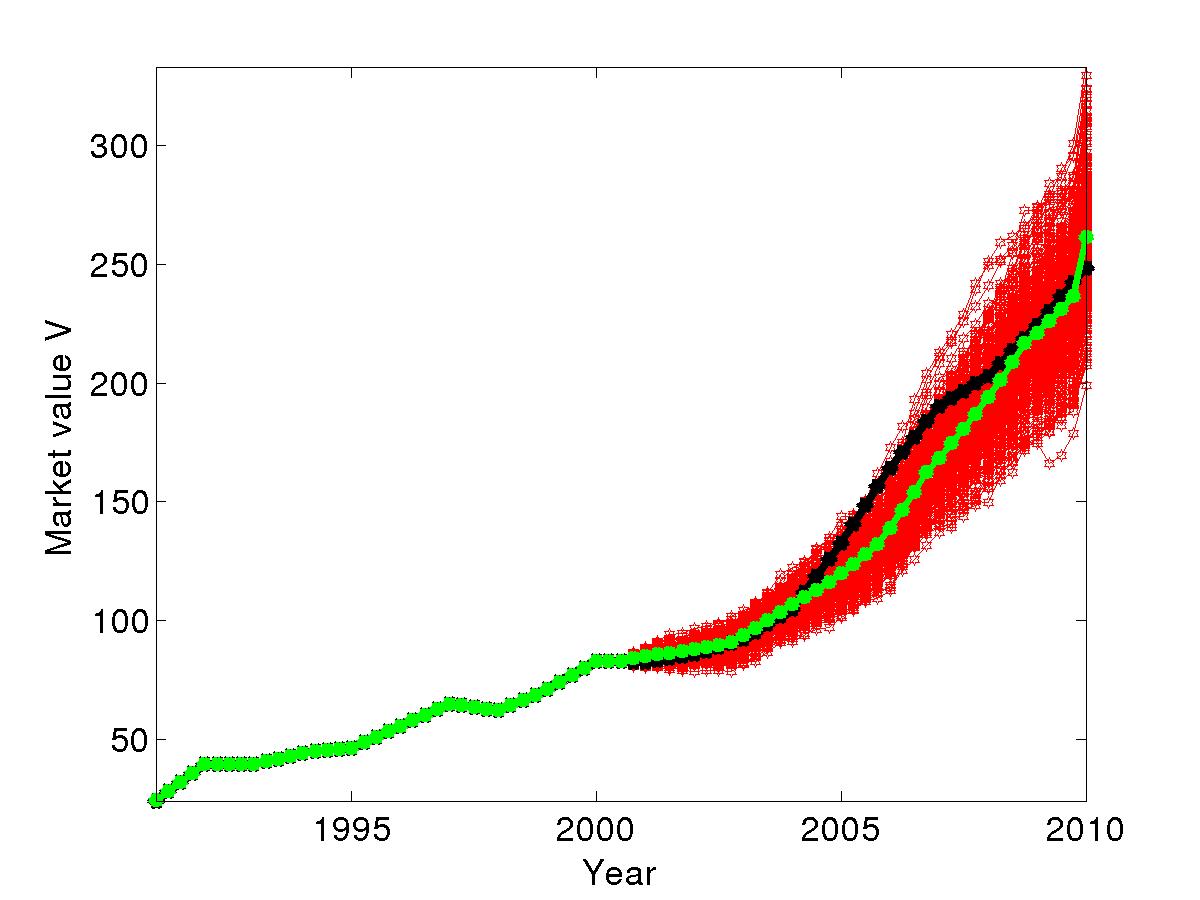
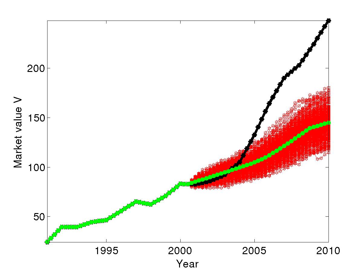
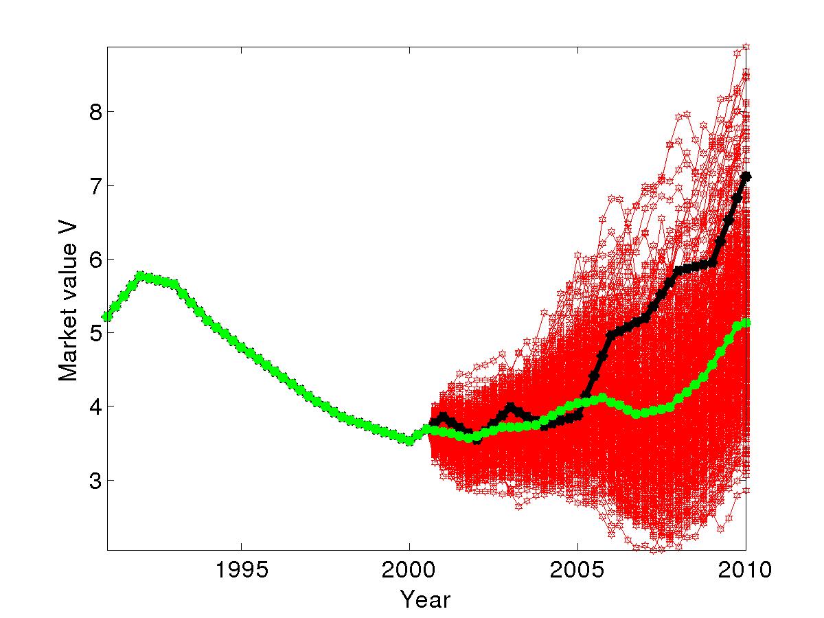
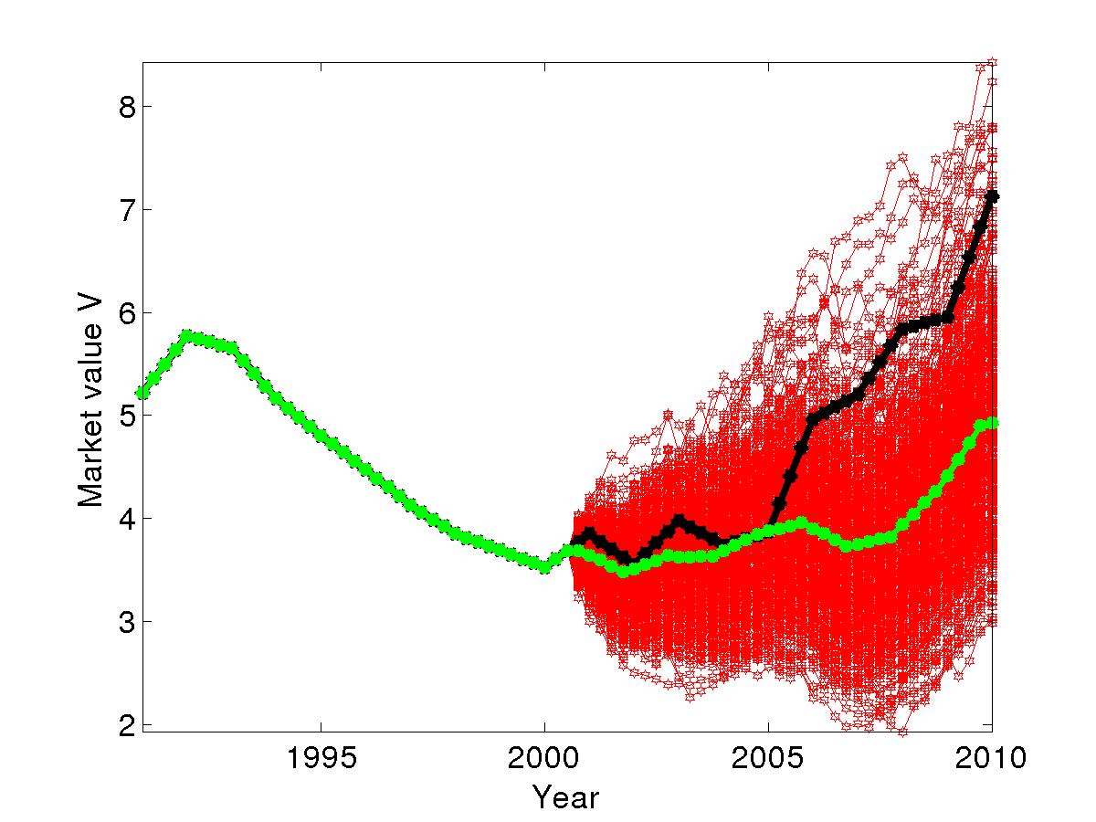
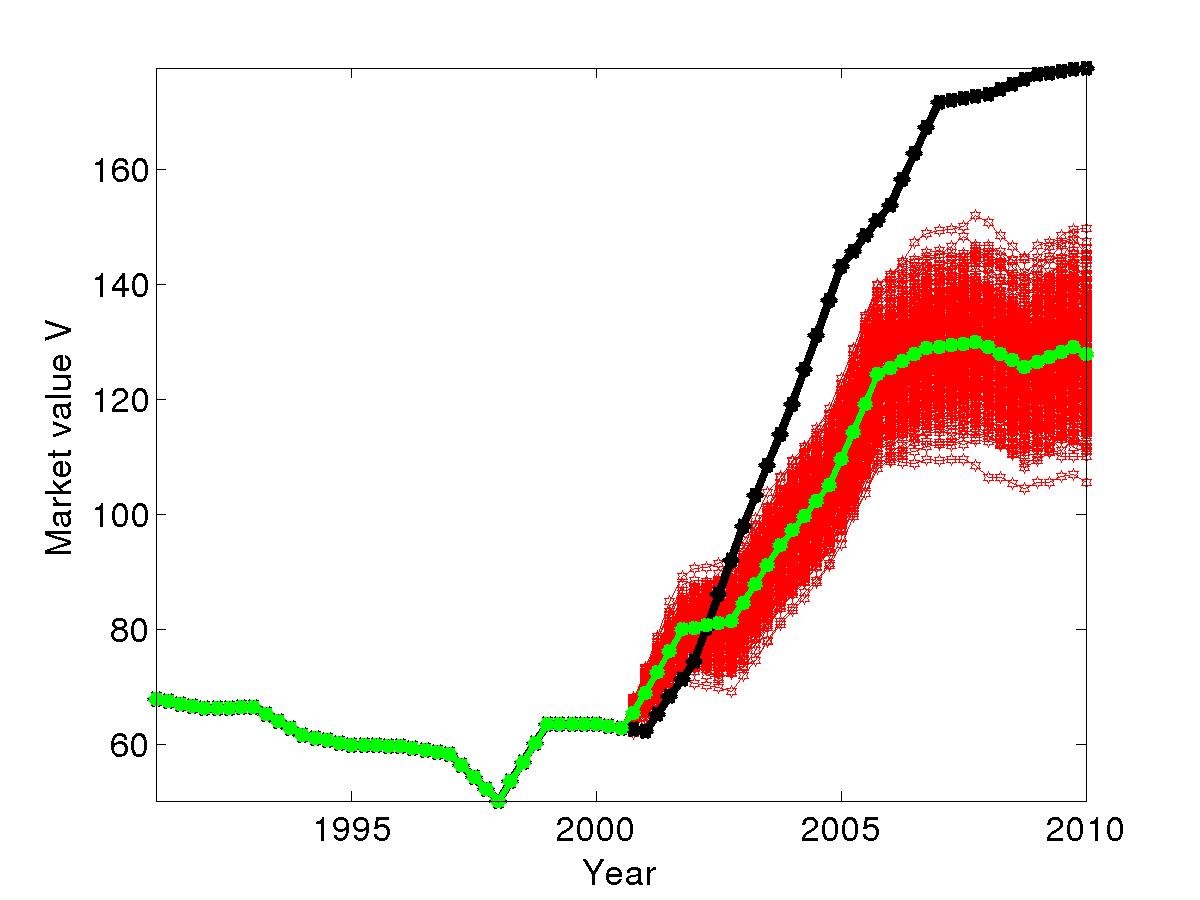
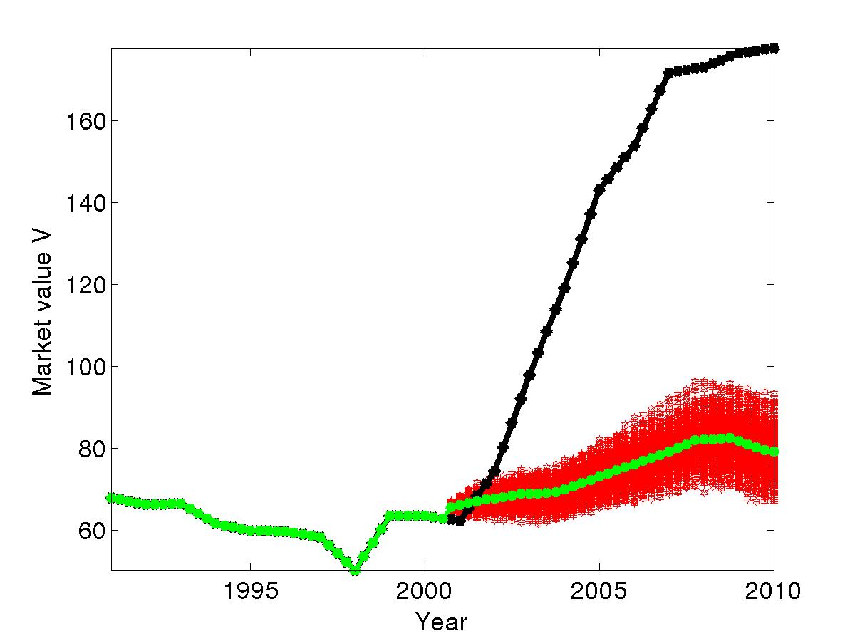
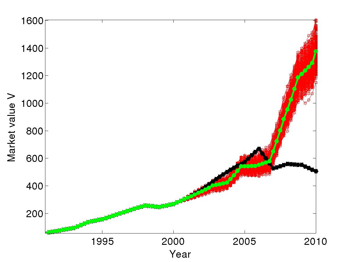
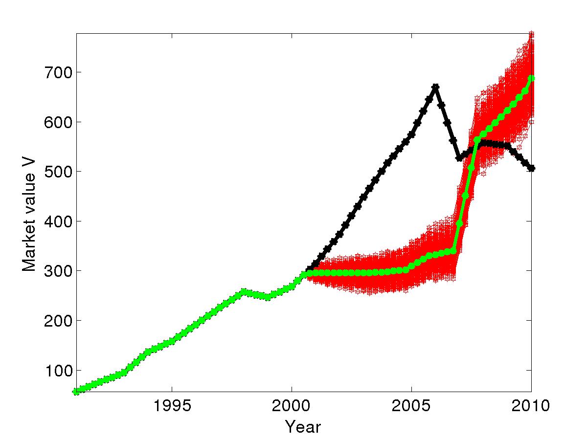
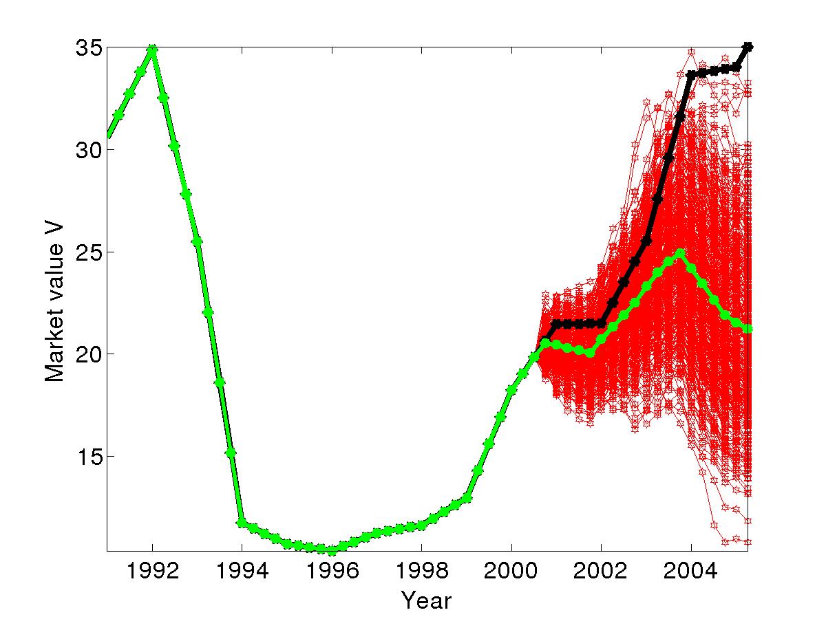
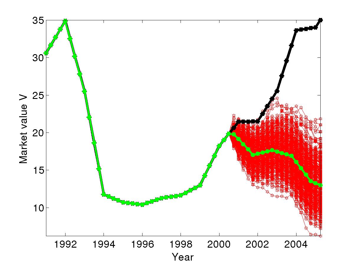
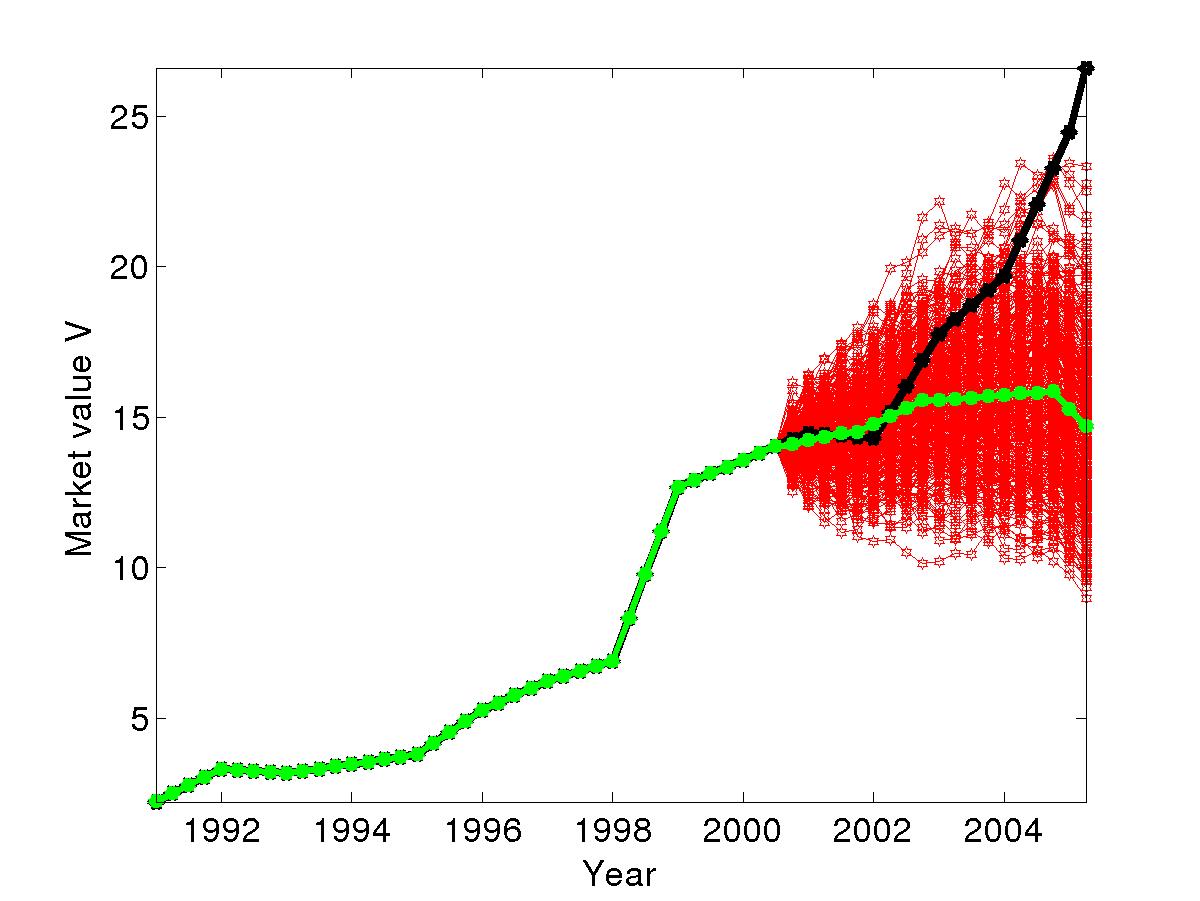
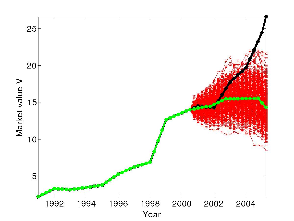
As we have already mentioned, the time origin corresponds to the year (2000+1/2), the data before are memory data and we want to predict the data after (2000+1/2). We plot 400 samples of the numerical solution for our delayed model and Merton model along with the means of the numerical samples (green curves). As the origin is year (2000+1/2), the part of the mean curves before the origin are just the curves of the real firm market value $V$ in that interval. The curves of the real firm market value $V$ as a function of time are in black (black thick curves). Indeed we want the means of the numerical samples (green curves) to fit well the real firm market value $V$ (black thick curves) with moderate standard derivations (few spread of the numerical samples comparing to its mean), this will be the aim of our comparisons.

In all graphs, the function $g$ (volatility in delayed model) is the quadratic interpolation of the standard deviation of daily returns $\sigma$ in the memory part while the volatility in the Merton model is just the mean of the memory part.

In Figure 1 we take $L=T=9.5$, the graphs at the left hand size. (Figure 1 and Figure 1 respectively for firms $C_{5}$ and $C_{4}$ ) correspond to the delayed model while the graphs at the right hand size (Figure 1 and Figure 1 respectively for firms $C_{5}$ and $C_{4}$) correspond to Merton model. For corporate $C_{5}$, Figure 1 shows the good prediction with reasonable standard deviation (as the numerical samples are not much spread) of the delay model while Figure 1 shows the early good prediction of the Merton model but the prediction has failled just after the year 2005. For corporate $C_{4}$, Figure 1 and Figure 1 show the good prediction before 2005 with relatively large standard deviation of the delayed model and Merton model.

In Figure 2, we aslo take $L=T=9.5$, the graphs at the left hand size (Figure 2 and Figure 2 respectively for firms $C_{3}$ and $C_{6}$) correspond to the delayed model while the graphs at the right hand size (Figure 2 and Figure 2 respectively for firms $C_{3}$ and $C_{6}$)) correspond to Merton model. For corporate $C_{3}$, Figure 2 shows an early accepted prediction for delayed model comparing to the Merton model in Figure 2 where the prediction is more bad (black thick curve been really far away from green curve). For corporate $C_{6}$, we have the same observation as for corporate $C_{3}$ according to Figure 2 and Figure 2.

In Figure 3 we take $L=9.5,\;T=5$, the graphs at the left (Figure 3 and Figure 3 respectively for firms $C_{1}$ and $C_{2}$) correspond to the delayed model while the graphs at the right (Figure 3 and Figure 3 respectively for firms $C_{1}$ and $C_{2}$) correspond to Merton model. From Figure 3, we can observe that for corporate $C_{1}$ the delayed model fit well the real data of the firm market value compared to the Merton model, while for corporate $C_{2}$ the two models fit well the real data of the firm market value before 2003.

3.3 Numerical Evaluation of Debt or Equity in a Levered Firm

3.3.1 Numerical schemes based on exponential integrators

Debt and equity are linked by relation (11), so we only need to solve one of the systems (23) and (33). We consider here the random partial differential (23), but where $C$, $C_{y}$ and $r$ are time depending functions. In our simulation we consider those values as time depending functions, which are constant within each year interval as we have in our data set. Indeed to solve numerically this equation the domain of $v$ need to be troncated. Taking in to account the fact that $C$, $C_{y}$ and $r$ are time depending functions, we therefore have

$$\left\{\begin{array}[]{l}\dfrac{1}{2}\,g^{2}(V(t-L))v^{2}\,f_{vv}+(r(t)v-C(t))f_{v}+f_{t}-r(t)f-C_{y}(t)+C(t)=0,\\ f(v,T)=\max(v-B,0),\;\;\;\;\;v\in[0,V_{\max}]\\ f(0,t)=0,\;\quad\quad\;\;\;t\in[T-L,T]\\ f(V_{\max},t)=V_{\max}-Be^{-\int_{t}^{T}r(s)ds},\;\quad\quad\;\;\;t\in[T-L,T]\end{array}\right.$$ (39)

Our model problem (39) is similar to Europeans call options prices, we can therefore take $V_{\max}$ three or four times $B$ according to [15]. In our simulation we take $V_{\max}=4B$, where $B$ is the amount that the firm must pay to the debtholders at the maturity date $T$ (like the strike price for options prices). Our system (39) is a backward system, to transform it to the forward one, we use the tranformation $\tau=T-t$, and the corresponding equation is given by

$$\left\{\begin{array}[]{l}\dfrac{1}{2}\,g^{2}(V(T-\tau-L))v^{2}\,f_{vv}+(r(\tau)v-C(\tau))f_{v}-r(\tau)f\\ \qquad\qquad\qquad\qquad\qquad\qquad\qquad\qquad\qquad-C_{y}(\tau)+C(\tau)=f_{\tau},\\ f(v,0)=\max(v-B,0),\;\;\;\;\;v\in[0,V_{\max}]\\ f(0,\tau)=0,\;\quad\quad\;\;\tau\in[0,L]\\ f(V_{\max},\tau)=V_{\max}-Be^{-\int_{T-\tau}^{T}r(s)ds},\;\quad\quad\;\;\;\tau\in[0,L]\end{array}\right.$$ (45)

Please note that after the transformation $\tau=T-t$, the functions $C(\tau),C_{y}(\tau)$ and $r(\tau)$ in (45) are normally the functions $C(T-\tau),C_{y}(T-\tau)$ and $r(T-\tau)$.

To apply sophistical technique to the convection term (the term with $f_{v}$) in order to avoid numerical instabilities, let us put this term in the so called the conservation form. In fact

$$(r(\tau)v-C(\tau))f_{v}=\left(r(\tau)v-C(\tau))f\right)_{v}-r(\tau)f$$

Using this relation, equation (45) become

$$\left\{\begin{array}[]{l}\dfrac{1}{2}\,g^{2}(V(T-\tau-L))v^{2}\,f_{vv}+\left((r(\tau)v-C(\tau))f\right)_{v}-2r(\tau)f,\\ \qquad\qquad\qquad\qquad\qquad\qquad\qquad\qquad\qquad-C_{y}(\tau)+C(\tau)=f_{\tau}\\ f(v,0)=\max(v-B,0),\;\;\;\;\;v\in[0,V_{max}]\\ f(0,\tau)=0,\;\quad\quad\;\;\tau\in[0,L]\\ f(V_{max},\tau)=V_{max}-Be^{-\int_{T-\tau}^{T}r(s)ds},\;\quad\quad\;\;\;\tau\in[0,L]\end{array}\right.$$ (51)

To solve equation (51) two cases can be considered:

1. The case where $T-\tau-L\leq 0,\;\;\;\forall\tau\in[0,L]$, then $T\leq L$.

2. The case where $T>L$.

For the first case ($T\leq L$) the RPDE (51) become the deterministic PDE since $V(t)=\varphi(t)\;\;$ for $t\in[-L,0]$ as given in (4).

For the second case ($T>L$), to solve (51) the following step should be followed

1. Solve the stochastic equation (4) to have a sample of the numerical solution of $V$ as we did in the previous section.
   

2. Use the numerical sample solution of $V$ from step 1 to build the diffusion coefficient (the coefficient of $f_{vv}$) in the RPDE (51), which therefore become a deterministic PDE for this fixed numerical sample of $V$.

3. Solve the deterministic PDE from step 2 for the fixed numerical sample of $V$ from step 1.

4. Repeat step 1, step 2 and step 3, $M$ times (relatively large) and use the Monte Carlo technique to estimate the expectation value of $f$ and also any moment of the stochastic process $f$ if need.

As the two cases require the solution of the deterministic PDE, in the sequel we will consider the first case ($T\leq L$), and the corresponding deterministic PDE is given by

$$\left\{\begin{array}[]{l}\dfrac{1}{2}\,g^{2}(\varphi(T-\tau-L))v^{2}\,f_{vv}+\left((r(\tau)v-C(\tau))f\right)_{v}-2r(\tau)f\\ \qquad\qquad\qquad\qquad\qquad\qquad\qquad\qquad\qquad-C_{y}(\tau)+C(\tau)=f_{\tau},\\ f(v,0)=\max(v-B,0),\;\;\;\;\;v\in[0,V_{max}]\\ f(0,\tau)=0,\;\quad\quad\;\;\tau\in[0,L]\\ f(V_{max},\tau)=V_{max}-Be^{-\int_{T-\tau}^{T}r(s)ds},\;\quad\quad\;\;\;\tau\in[0,L].\end{array}\right.$$ (57)

For the discretization in the direction of $v$, we use the combined finite difference–finite volume method. The interval $[0,V_{max}]$ is subdivised into $N$ parts that we assume equal without loss the generality. As in center finite volume method, we approximate $f$ at the center of each interval. The diffusion part of the equation is approximated using the finite difference while the convection term is approximated using the standard upwinding usual used in porous media flow problems [19, 1, 18, 20].

Let

$$v_{i}=(2i-1)h/2,\;\;\;h=\dfrac{V_{max}}{N},\;\;\ i=1,2,.....,N$$

being the center of each subdivision . We approximate the diffusion term at each center by

$$\dfrac{1}{2}\,g^{2}(\varphi(T-\tau-L))v_{i}^{2}\,f_{vv}(v_{i}) \approx \dfrac{1}{2h^{2}}\,g^{2}(\varphi(T-\tau-L))v_{i}^{2}\times$$

$$\left(f_{i+1}(\tau)-2f_{i}(\tau)+f_{i-1}(\tau)\right),\;i=2,...,N-1.$$

$$\dfrac{1}{2}\,g^{2}(\varphi(T-\tau-L))v_{1}^{2}\,f_{vv}(v_{1}) \approx \dfrac{2}{3h}\,g^{2}(\varphi(T-\tau-L))v_{1}^{2}\times$$

$$\left(\dfrac{f_{2}(\tau)-f_{1}(\tau)}{h}-2\dfrac{f_{1}(\tau)}{h}\right)$$

$$\dfrac{1}{2}\,g^{2}(\varphi(T-\tau-L))v_{N}^{2}\,f_{vv}(v_{N}) \approx \dfrac{2}{3h}\,g^{2}(\varphi(T-\tau-L))v_{N}^{2}\times$$

$$\left(\dfrac{f(V_{max},\tau)-f_{N}(\tau)}{h/2}-\dfrac{f_{N}(\tau)-f_{N-1}(\tau)}{h}\right)$$

This approximation is similar to the one in [21] with central difference on non uniform grid. We approximate the convection term using the standard upwinding technique as following

$$\left(r(\tau)v-C(\tau))f\right)_{v}(v_{i})\approx\dfrac{(r(\tau)v_{i+1/2}-C(\tau))f_{i}^{+}(\tau)-(r(\tau)v_{i-1/2}-C(\tau))f_{i-1}^{+}(\tau)}{h}$$

where

$$f_{i}^{+}(\tau) = \left\{\begin{array}[]{l}f_{i}(\tau)\;\;\;\;\;\text{if}\;\;\;\;r(\tau)v_{i+1/2}-C(\tau)\geqslant 0\\ f_{i-1}(\tau)\;\;\;\;\;\text{if}\;\;\;\;r(\tau)v_{i+1/2}-C(\tau)<0\end{array}\right.$$ (60)

$$v_{i+1/2} = v_{i}+h/2,\;\;\;\;v_{i-1/2}=v_{i}-h/2=v_{i-1}+h/2,$$ (61)

where

$$f_{i}(\tau)\approx f(v_{i},\tau).$$

Reorganizing all previous diffusion and convection approximations lead to the following initial value problem

$$\left\{\begin{array}[]{l}\dfrac{d\mathbf{f}}{d\tau}=\mathbf{A}(\tau)\mathbf{f}+\mathbf{b}(\tau),\;\;\;\;\;\;\tau\in[0,L]\\ \mathbf{f}(0)=\left(\max(v_{1}-B,0),...,\max(v_{N}-B,0)\right)^{T}.\end{array}\right.$$ (64)

where $\mathbf{A}(\tau)$ is a tridiagonal matrix and

$$\mathbf{f}(\tau)=\left(f_{i}(\tau)\right)_{1\leq i\leq N},\mathbf{b}(\tau)=C(\tau)-C_{y}(\tau)+\mathbf{k}(\tau).$$ (65)

where $\mathbf{k}$ is the contribution from boundary conditions.

The function $x\mapsto\max(x,0)$ is not smooth, it important to approximate it by a smooth function. The approximation in [21] is a fourth-order smooth function denoted $\pi_{\epsilon}$ and defined by

$$\pi_{\epsilon}(x)=\left\{\begin{array}[]{l}x\;\;\;\;\text{if}\;\;\;\;\;\;x\geqslant\epsilon\\ c_{0}+c_{1}x+.....+c_{9}x^{9}\;\;\;\;\text{if}\;\;\;\;\;\;-\epsilon<x<\epsilon\\ 0\;\;\;\;\text{if}\;\;\;\;\;x\leq-\epsilon\end{array}\right.$$ (69)

where $0<\epsilon\ll 1$ is the transition parameter and

$$c_{0}=\dfrac{35}{256}\epsilon,\;\;\;\;c_{1}=\dfrac{1}{2},\;\;\;c_{2}=\dfrac{35}{64\epsilon},\;\;\;\;c_{4}=-\dfrac{35}{128\epsilon^{3}},\,\,\,$$

$$c_{6}=\dfrac{7}{64\epsilon^{5}},\,\,c_{8}=-\dfrac{5}{256\epsilon^{7}},\;\;c_{3}=c_{5}=c_{7}=c_{9}=0.$$

This approximation allow us to write

$$\mathbf{f}(0)=\pi_{\epsilon}(\mathbf{v}-B),\;\;\;\mathbf{v}=\left(v_{i}\right)_{1\leq i\leq N}.$$ (70)

Let us introduce the time stepping discretization for the ODE (64) based on exponential integrators. Classical numerical methods usually used are Implicit Euler scheme and Crank–Nicolson scheme [22]. Following works from [21, 19, 1] the exact solution of (64) is given by

$$\mathbf{f}(\tau_{n}+\Delta\tau) = e^{\int_{\tau_{n}}^{\tau_{n}+\Delta\tau}\mathbf{A}(s)ds}\left[\mathbf{f}(\tau_{n})+\int_{\tau_{n}}^{\tau_{n}+\Delta\tau}e^{-\int_{\tau_{n}}^{s}\mathbf{A}(y)dy}\mathbf{b}(s)ds\right]$$ (72)

$$\qquad\qquad\tau_{n}=n\,\Delta\tau,\;\;\;\;\;n=0,...,M,\;\;\;\;\ \Delta\tau>0.$$

Note that (72) is the exact representation of the solution, to have the numerical schemes, approximations are needed, the first approximations (using the quadrature rule) may be

$$\int_{t_{n}}^{t_{n}+\Delta\tau}\mathbf{A}(s)ds\approx\Delta\tau\mathbf{A}(\tau_{n})\;\;\;\;\int_{\tau_{n}}^{s}\mathbf{A}(y)dy\approx(s-\tau_{n})\mathbf{A}(\tau_{n})$$ (73)

Using these approximations we therefore have the following second-order approximation

$$\mathbf{f}(\tau_{n}+\Delta\tau) \approx e^{\Delta\tau\mathbf{A}(\tau_{n})}\left[\mathbf{f}(\tau_{n})+\int_{\tau_{n}}^{\tau_{n}+\Delta\tau}e^{-(s-\tau_{n})\mathbf{A}(\tau_{n})}\mathbf{b}(s)ds\right]$$ (74)

The simple scheme called Exponential Differential scheme of order 1 (ETD1) is obtained by approximating $\mathbf{b}(s)$ by the constant $\mathbf{b}(\tau_{n})$ and is given by

$$\mathbf{f}_{n+1}=\mathbf{f}_{n}+\left(\Delta\tau\mathbf{A}(\tau_{n})\right)^{-1}\left[\mathbf{A}(\tau_{n})\mathbf{f}_{n}+\mathbf{b}(\tau_{n})\right].$$ (75)

A second order scheme is given in [21].

Following the work in [23, Lemma 4.1], if the the function $\mathbf{b}$ can be well approximated by the polynomial of degree $p$ (which is the case here since we have the exponential decay at the boundary $v=V_{max}$), from (74) we have

$$\mathbf{f}_{n+1}=\varphi_{0}(\Delta\tau\mathbf{A}(\tau_{n}))\mathbf{f}_{n}+\underset{j=0}{\sum^{p-1}}\underset{l=0}{\sum^{j}}\dfrac{\tau_{n}^{j-l}}{(j-l)!}\Delta\tau^{l+1}\varphi_{l+1}(\Delta\tau\mathbf{A}(\tau_{n}))\mathbf{b}_{j+1},$$ (76)

where

$$\mathbf{b}(\tau) \approx \underset{j=0}{\sum^{p-1}}\dfrac{\tau^{j}}{j!}\mathbf{b}_{j+1},$$

$$\varphi_{0}(x) = e^{x},\;\;\;\varphi_{l}(x)=x\varphi_{l+1}(x)+\dfrac{1}{l!},\,\;\;\;l=0,1,2,.....$$

Note that to have high order accuracy in time for $p>2$, the integral in (73) should be approximated more accurately. The Magnus expansion may also used in such case.

3.3.2 Application with corporate data

All schemes here can be implemented using Krylov subspace technique in the computation the expomential functions presented in those schemes with the Matlab functions expmvp.m or phipm.m from [23, 24]. The Krylov subspace dimension we use is $m=10$ and the tolerance using in the computation of the expomential functions $\varphi_{i}$ is $tol=1e-6$. We use $p=2$ and obtain second order accuracy in time as the approximations (73) are second order in time.

We used the following frims:

• Magna International Inc (Figure 4)

• First Citizens Bancshares Inc NC (Figure 5)

• Coca-Cola CO (Figure 6)

• One Liberty Properties INC (Figure 7)

• Cisco Systems INC (Figure 8)

• C B S Corp NEW (Figure 9)

• Nam Tai Electronics INC (Figure 10)

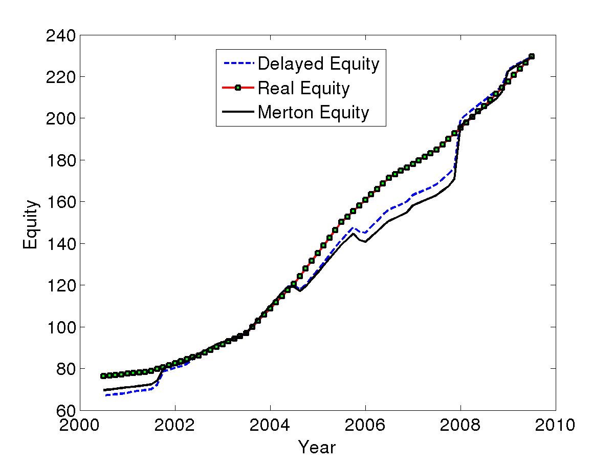
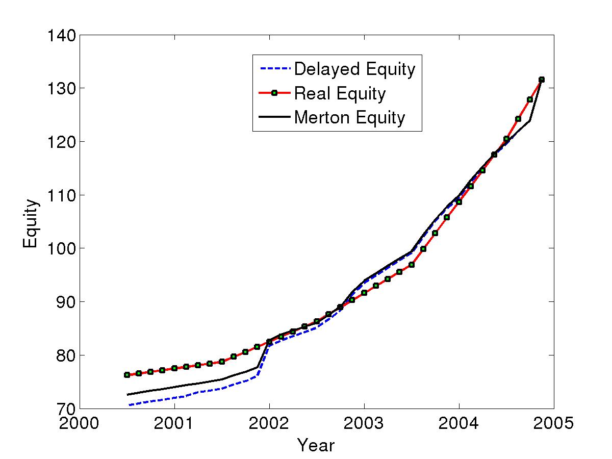
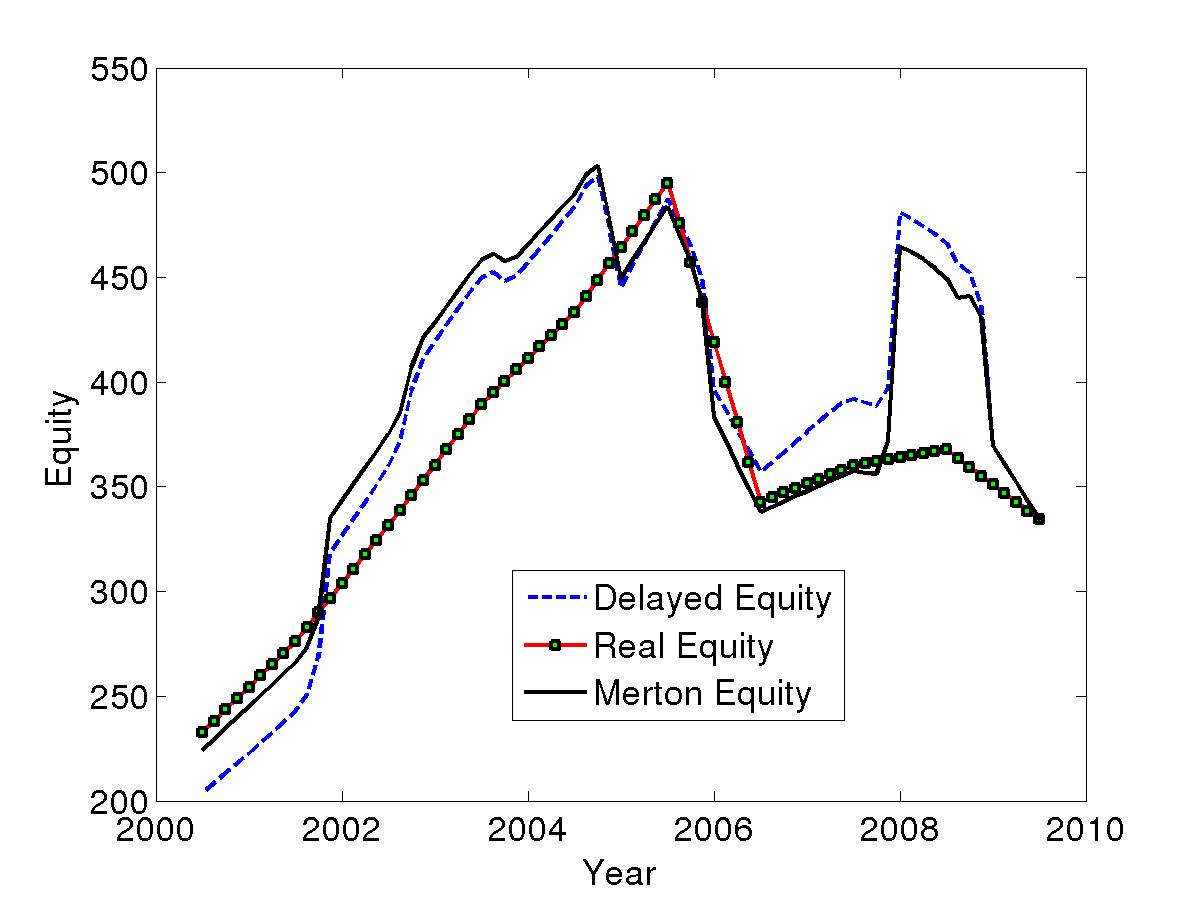
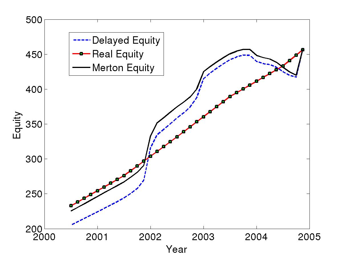
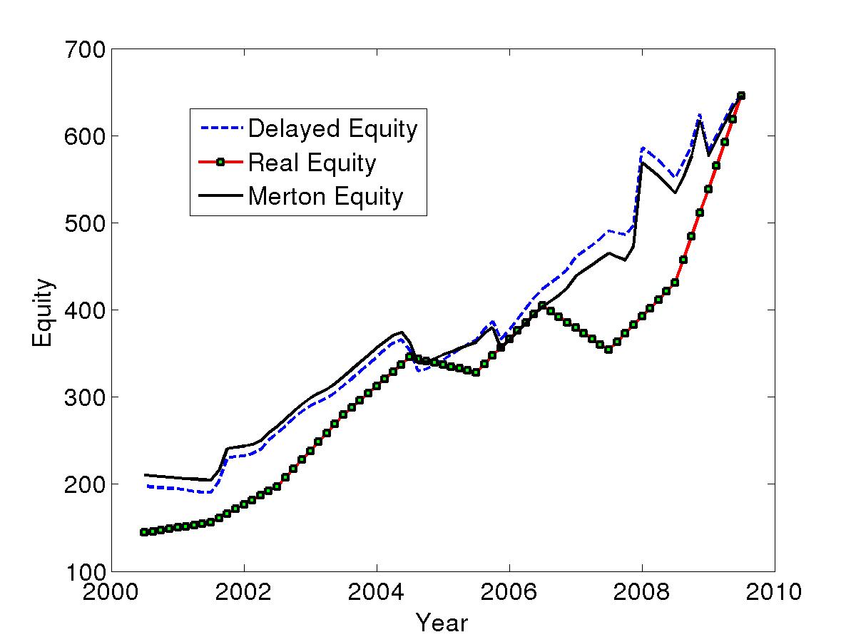
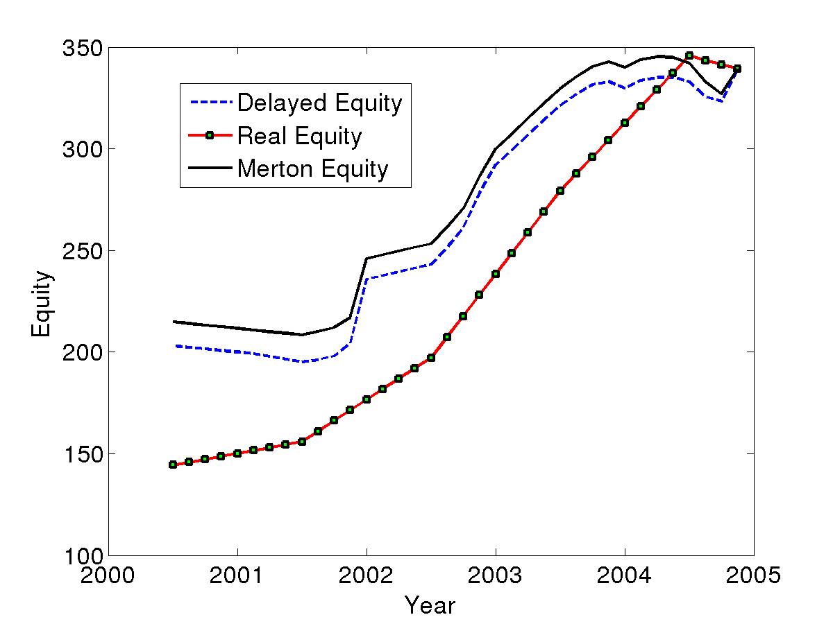
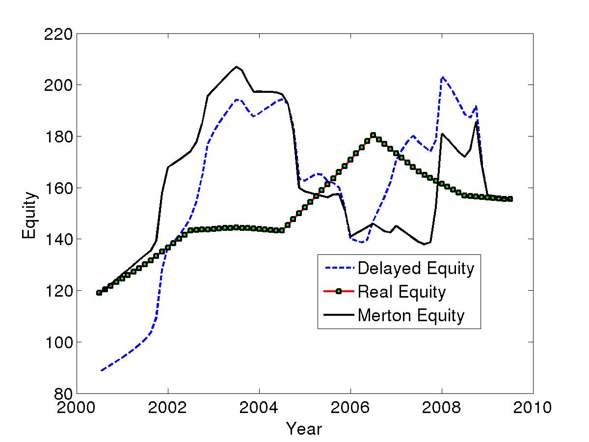
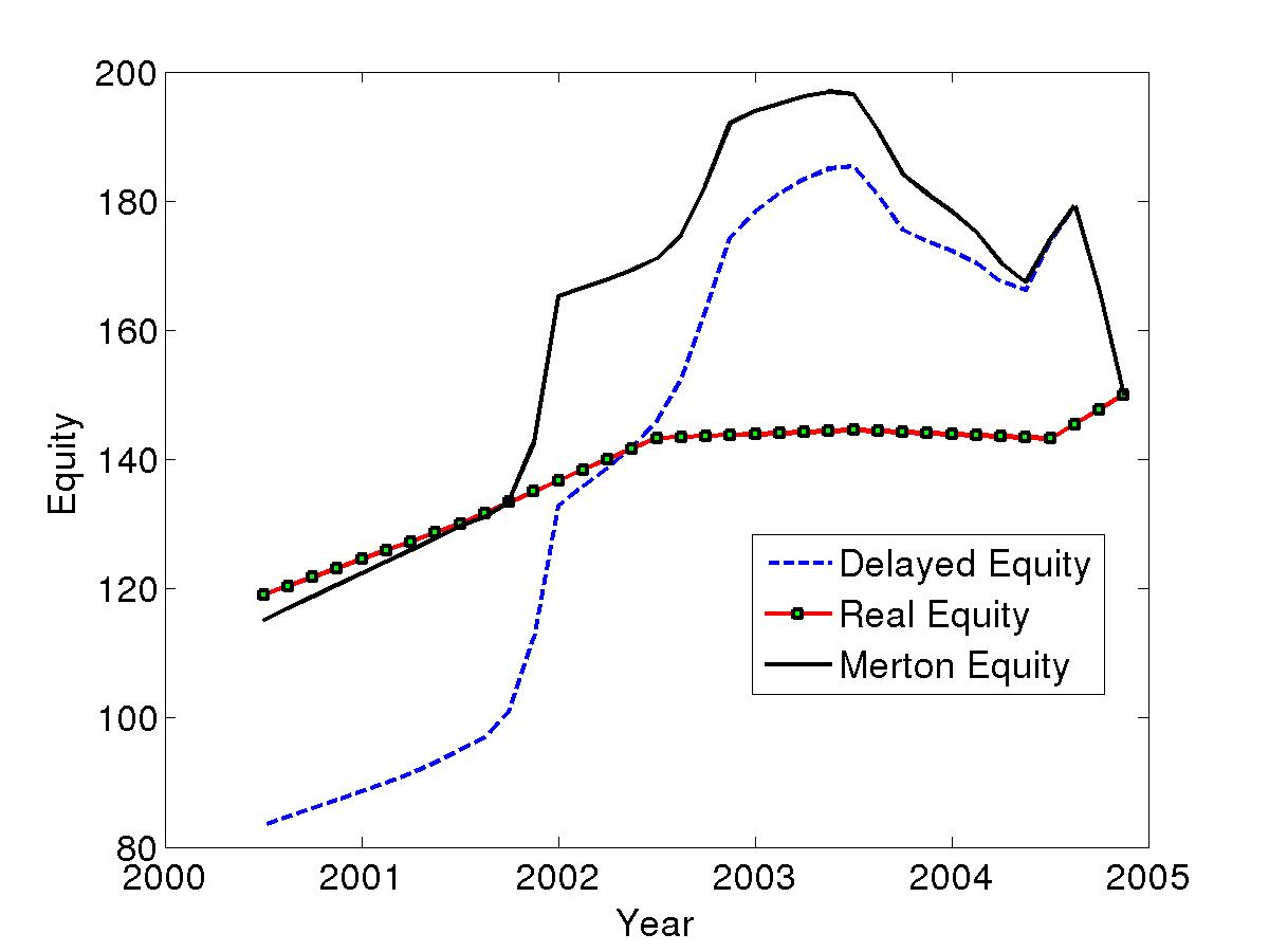
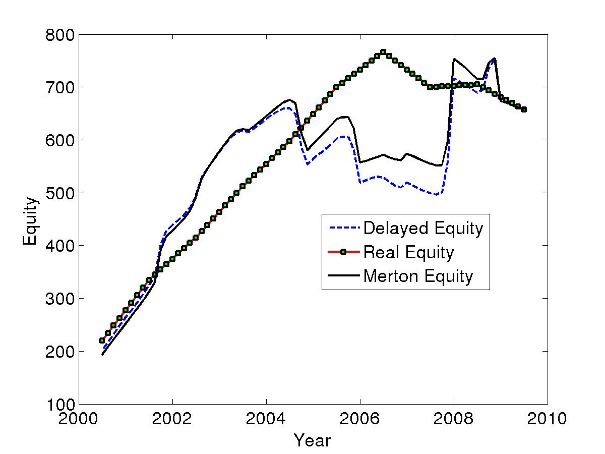
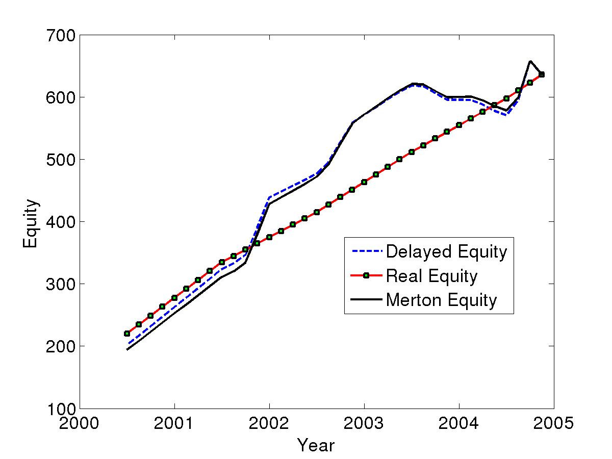
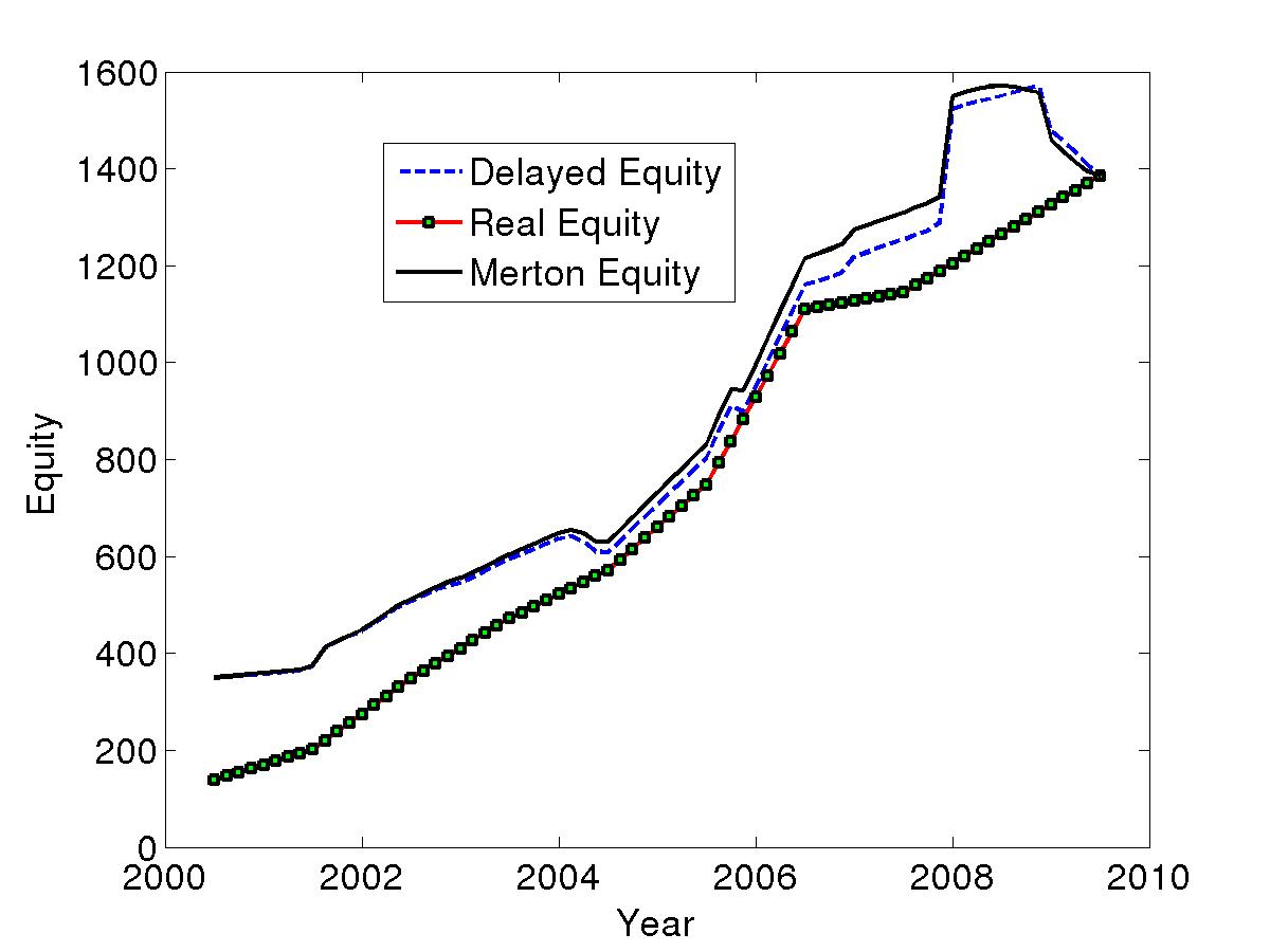
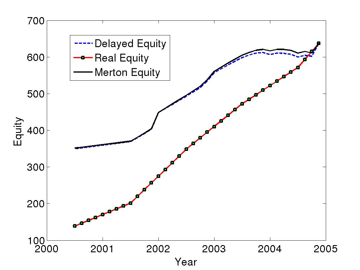
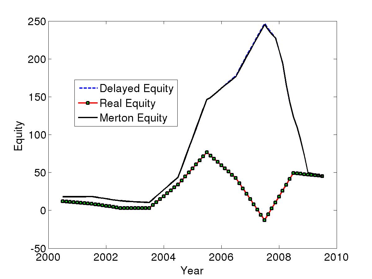
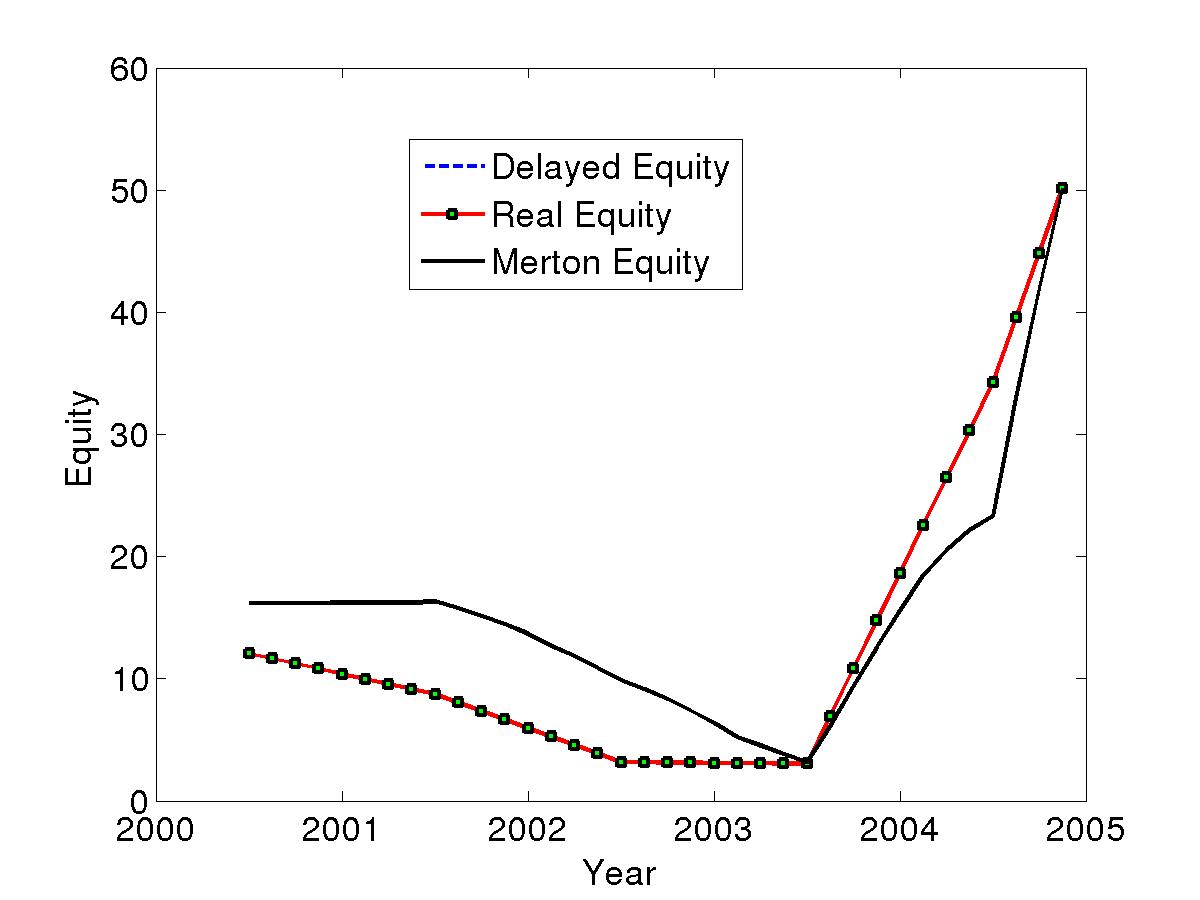
Here again, the time origin corresponds to the year (2000+1/2), the data before are memory data and we want to predict the data after (2000+1/2). In the legends of all of our graphs we use the following notation

• “Delayed Equity” is for the numerical equity value from our nonlinear delayed model.

• “Real Equity” is for the real equity value of the corporate.

• “Merton Equity” is for the numerical equity value from Merton model.

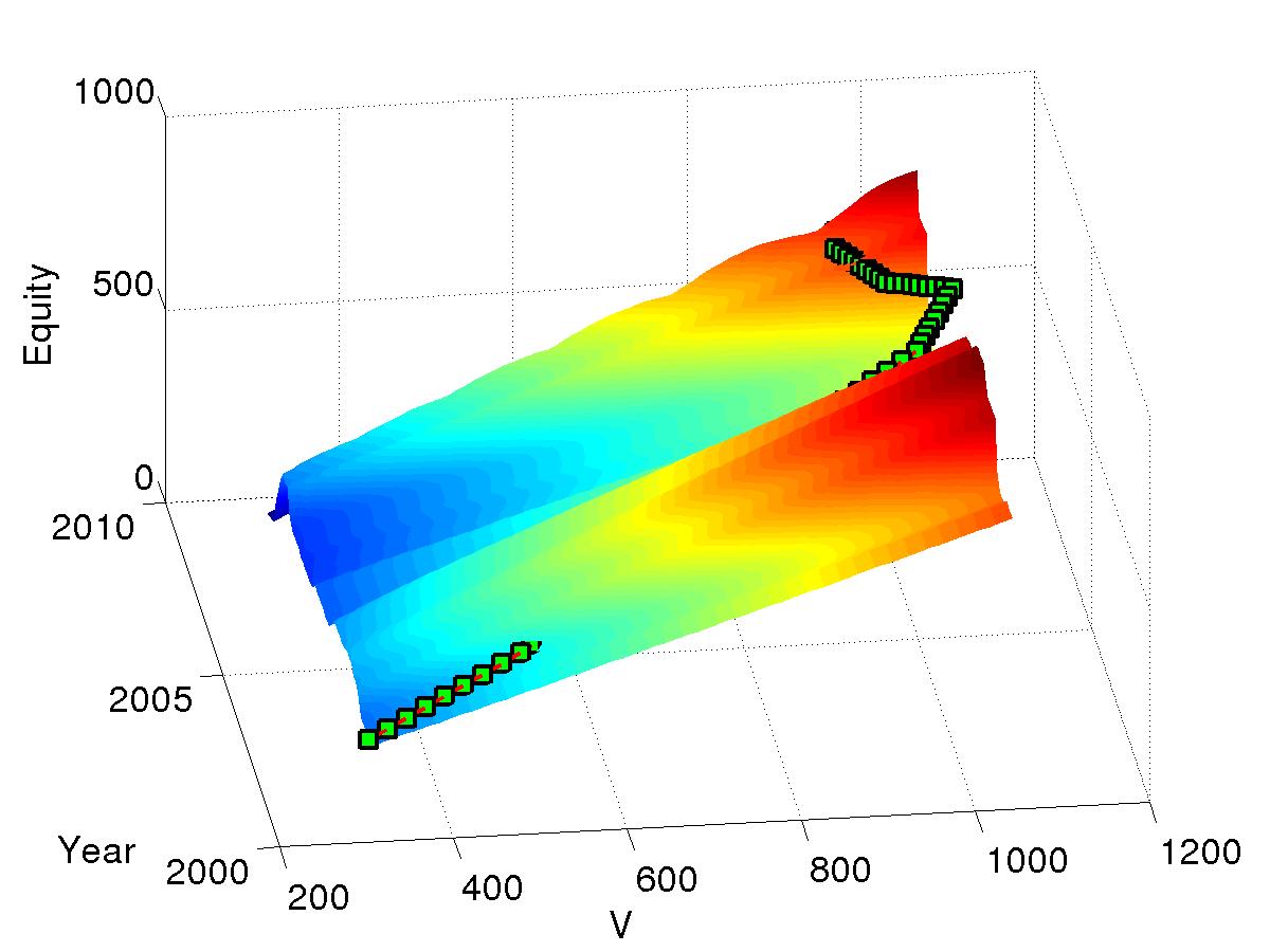
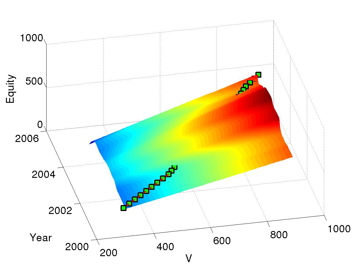
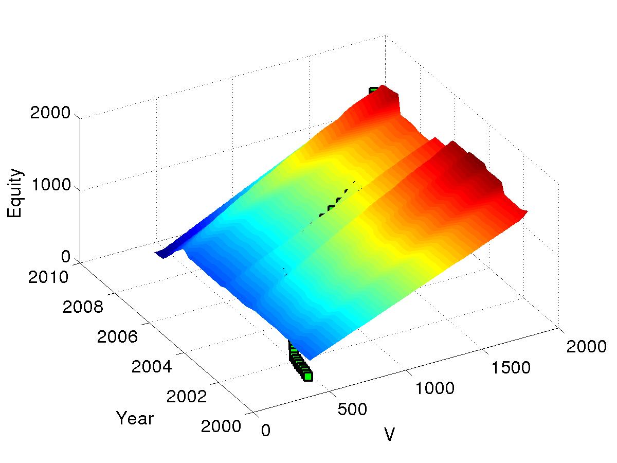
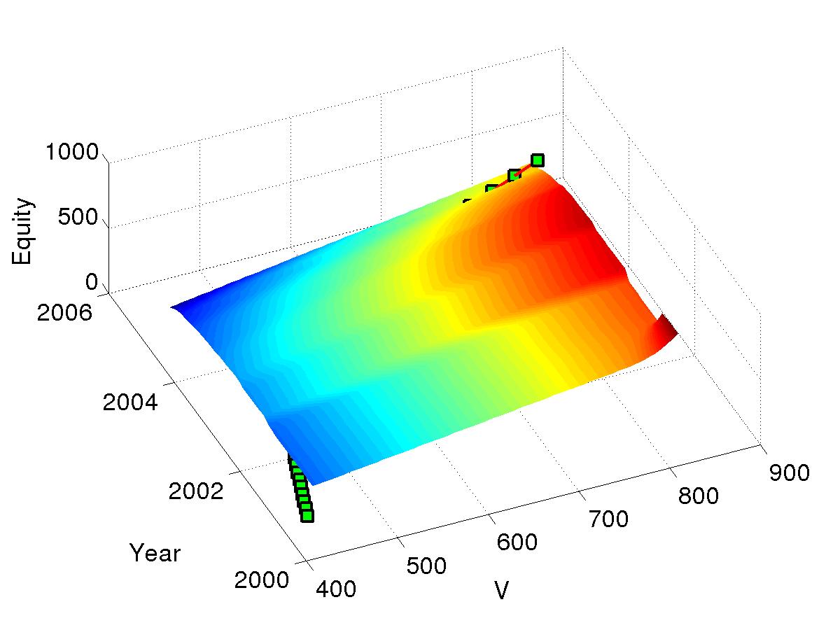
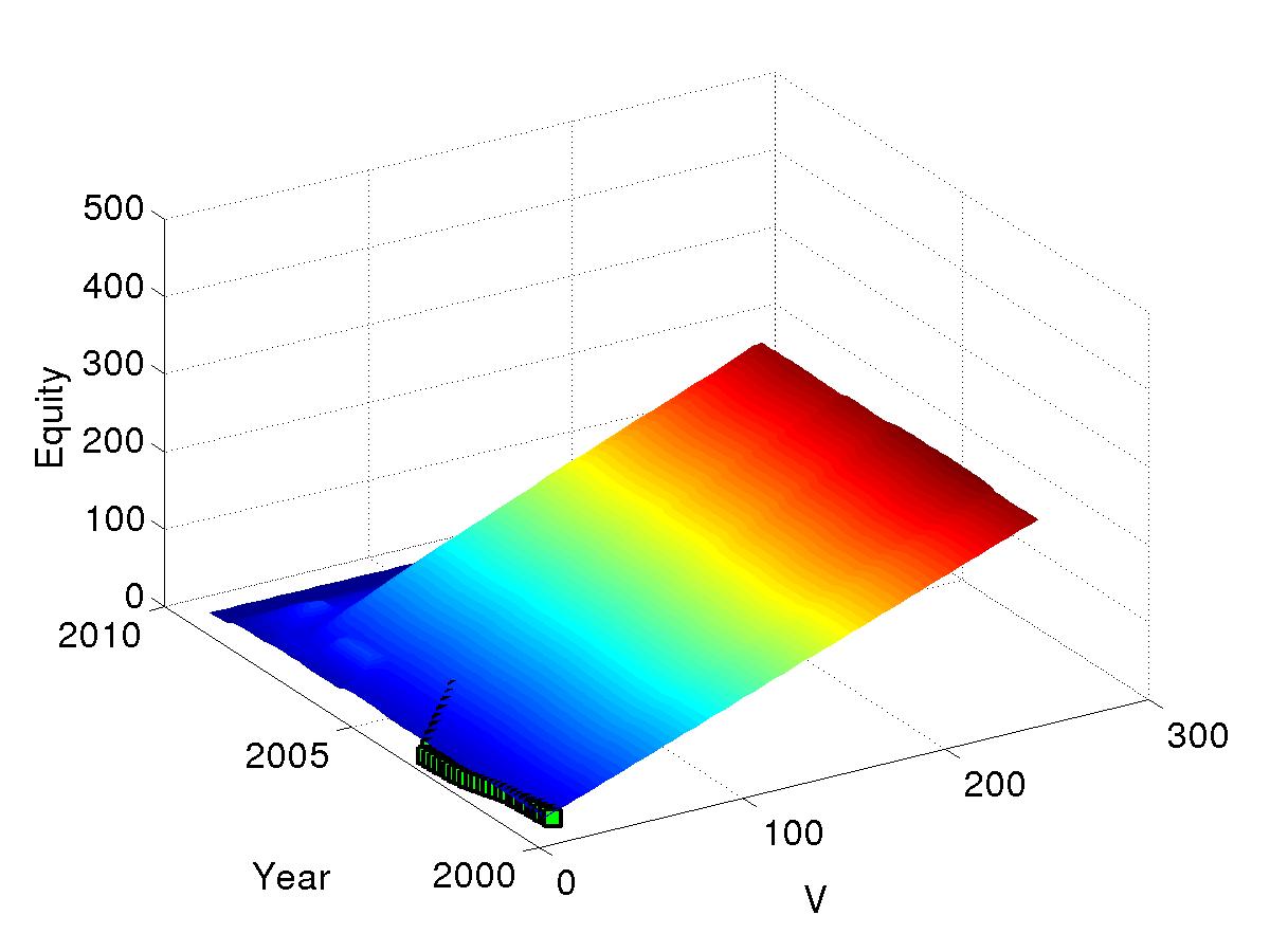
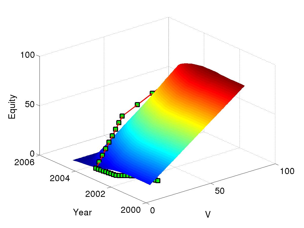
In our surface graphs of the numerical equity value, we plot only the part where the variable $V$ is between the minimun and the maximum values of our real market value $V$. In all simulations with our delayed model, we take $L=9.5$. In all graphs, the function $g$ (volatility in delayed model) is the quadratic interpolation of the standard deviation of daily returns $\sigma$ in the memory part while the volatility in the Merton model is just the mean of the memory part.

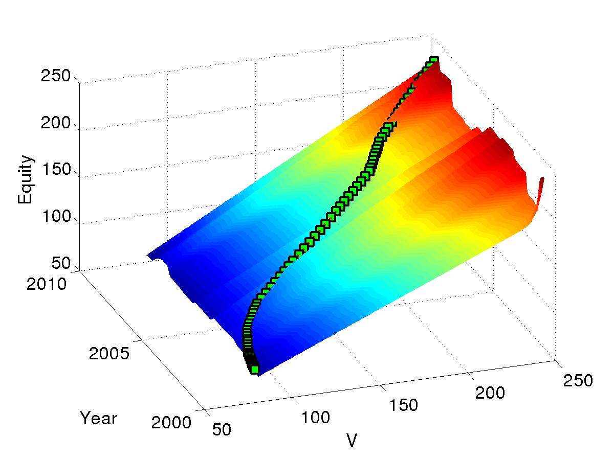
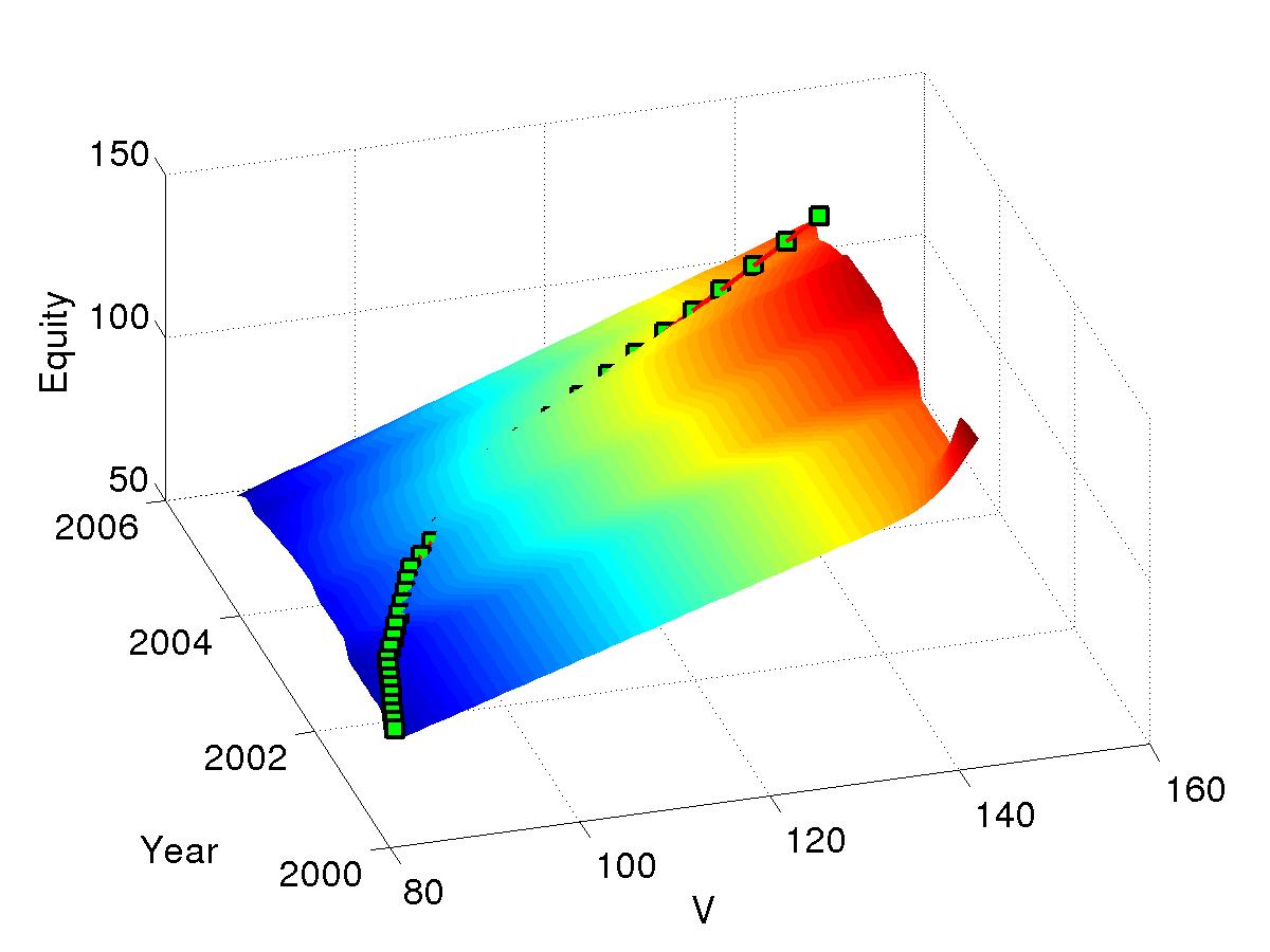
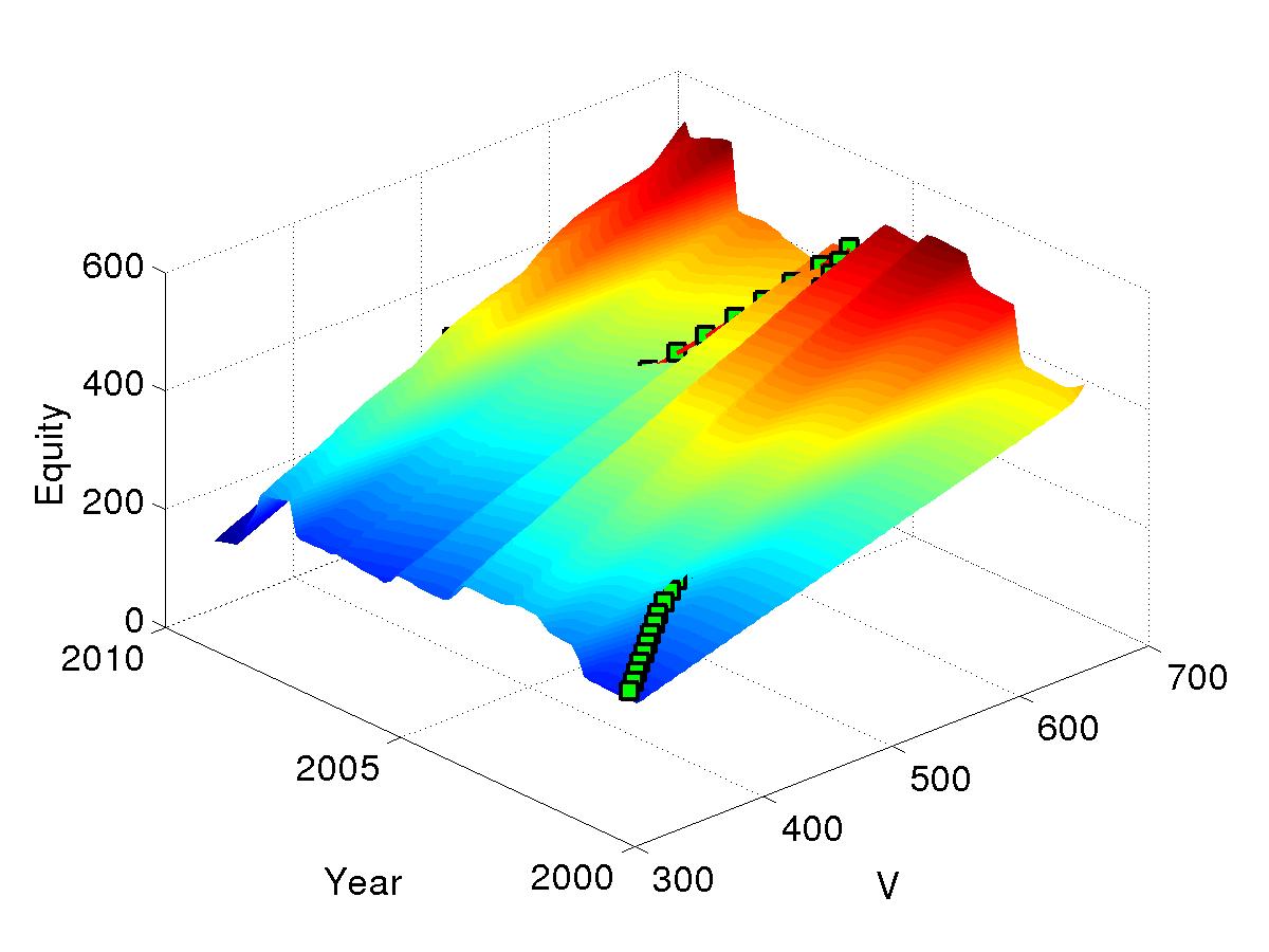
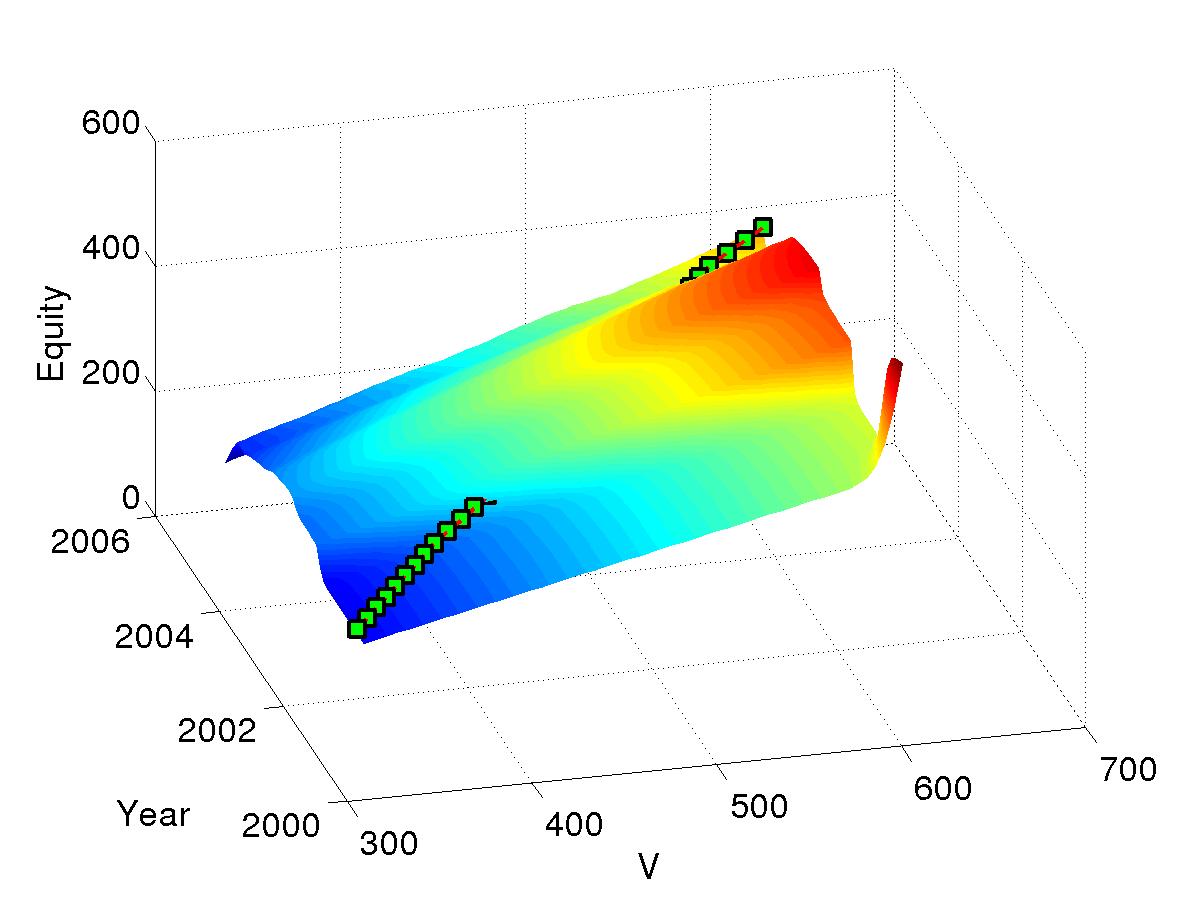
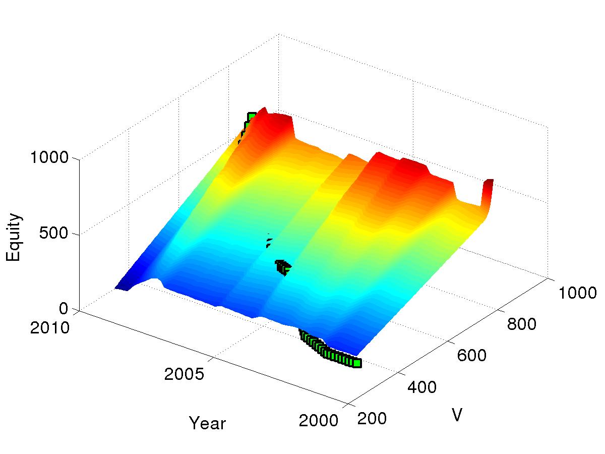
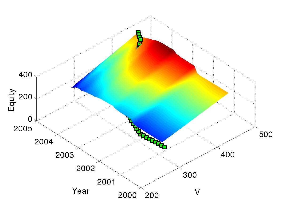
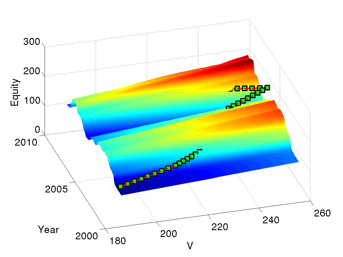
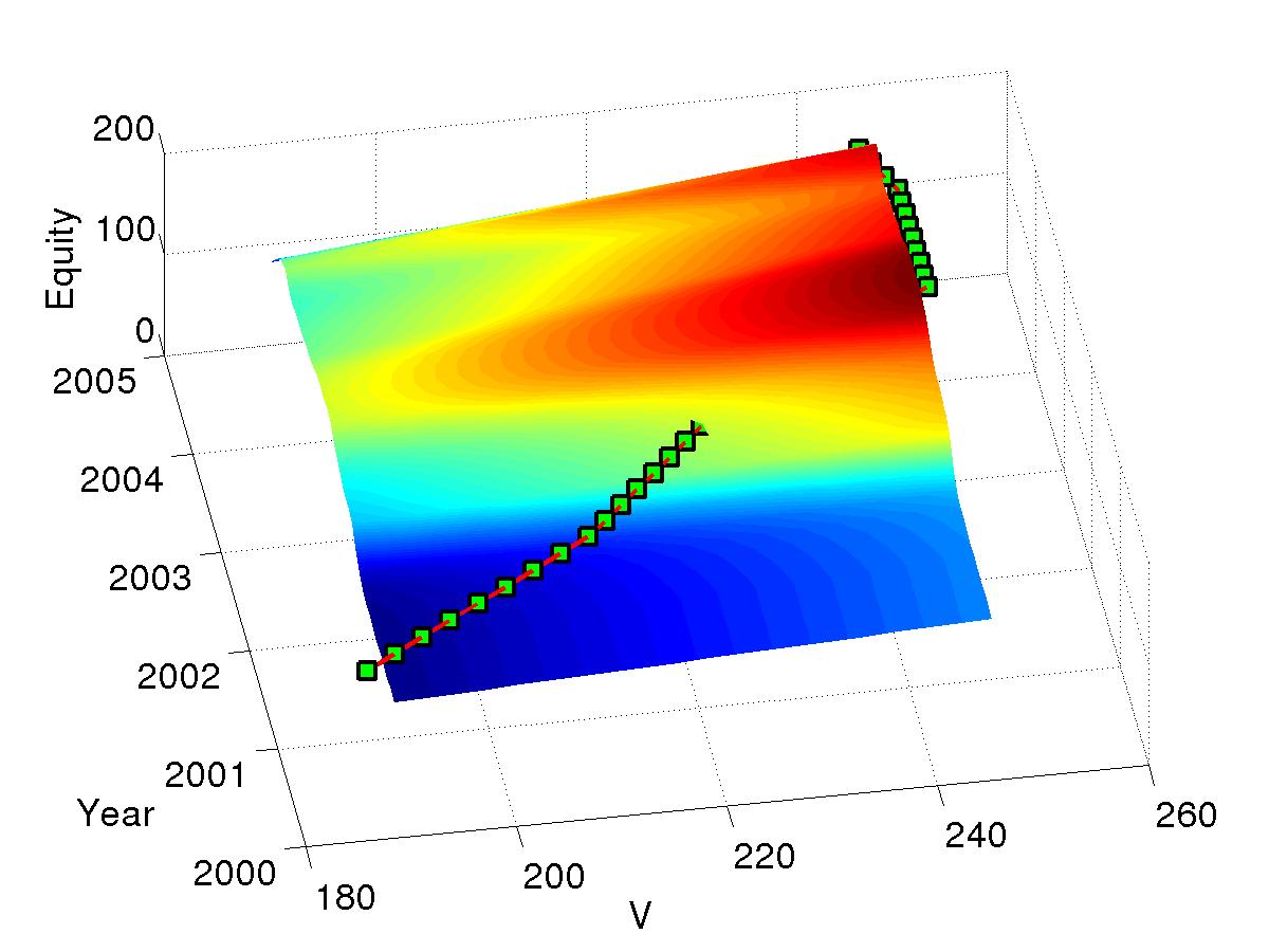
For each firm, we plot at the left hand size both the surface graphs of the numerical equity value from our delayed model at $T=9.5$ and $T=5$. In those 3D surface graphs, we also plot the corresponding 3 D graphs (green curves) of the real data of the firm equity value as a function of the time (year) and $V$. At the right hand size, we plot in 2 D the firm equity value as a function of time (year), corresponding to the surface graphs at the left hand size. Those 2 D equity graphs contain the numerical equity value from our delayed model, the numerical equity value of the Merton model and the real data equity value of the firm.

In our simulations, for a given $T$, the promised debt $B$ is just the real debt value of the firm at time $T$.

For firm $C_{5}$ in Figure 4, we can observe that both the delayed model and Merton model fit well the real market equity value of the firm. The accuracy of the two methods varies within some time interval as we can observe in Figure 4 and Figure 4.

For firm $C_{6}$ in Figure 5, comparing to firm $C_{5}$ the two models fit less. In a wide time interval in Figure 5 and Figure 5, the delayed model is more close to the real market equity of the firm. We can also observe a good early fit in the Merton model.

For firm $C_{7}$ in Figure 6, comparing to firm $C_{5}$ the two models fit less. But for the maturity date $T=9.5$ in Figure 6 the fitting is relatively good for the two models. The accuracy of the two methods varies within some time interval as we can observe in Figure 6 and Figure 6.

For firm $C_{8}$ in Figure 7, the fitting is relatively bad for the two models. However we can observe in Figure 7 and Figure 7 the good early fit in the Merton model, and that in the wide time interval the delayed model is more close to the real market equity of the firm than the Merton model.

For firm $C_{9}$ in Figure 8, the fitting is relatively good for the two models in the early time interval and become relatively bad just after.

For firm $C_{10}$ in Figure 9, the fitting is relatively good for the two models for the maturity date $T=9.5$ in Figure 9 at the middle time interval and bad for the maturity date $T=5$ in Figure 9.

For firm $C_{11}$ in Figure 10, the fitting is relatively good for the two models in the early time interval but become bad just after. The two models are confused.

4 Conclusion

In this paper, numerical techniques to solve delayed nonlinear model for pricing corporate liabilities are provided. The numerical technique to solve the RPDEs modeling debt and equity value combines the finite difference–finite volume methods (discretization respect to the firm value $V$) and an exponential integrator (discretization respect to the time $t$). The matrix exponential functions are computed efficiently using Krylov subspace technique.

Using financial data from some firms, we compare numerical solutions from both our nonlinear model and classical Merton to the real firm’s data. This comparaison shows that our nonlinear model behaves very well. We conclude that in corporate finance the past dependence of the firm value process may be an important feature and therefore should not be ignored.

References

- [1] A. Tambue, G. J.Lord, and S. Geiger, An exponential integrator for advection-dominated reactive transport in heterogeneous porous media. Journal of Computational Physics , 229(10):3957–3969, 2010.
- [2] S. Gryglewicz, A Theory of Corporate Financial Decisions with Liquidity and Solvency Concerns journal of Financial Economics 99, 365–384, 2011.
- [3] B. Dumas, J. Fleming and R. E. Whaley, Implied Volatility Functions: Empirical Tests. The Journal of finance, 53 , No 6, 2059–2106, 1998.
- [4] D. S. Bates, Testing Option Pricing Models, Statistical Models in Finance. Handbook of Statistics North-Holland, Amsterdam, 14 (1996), 567–611.
- [5] L. O. Scott, Option Pricing when the Variance Changes Randomly: Theory, Estimation and an Application. J. Financial Quant. Anal, 22, 419–438,1987.
- [6] R. C. Blattberg, and N. J. Gonedes, A Comparison of the Stable and Student Distributions as Statistical Models for Stock Prices. J. Business, 47 , 244–280,1974
- Merton, [1974] R. C. Merton, On the Pricing of Corporate Debt: The Risk Structure of Interest Rates. Journal of Finance, 29:449–470, 1974.
- Merton, [1977] R. C. Merton, An Analytic Derivation of the Cost of Deposit Insurance and Loan Guarantees. Journal of Banking and Finance, 9:3–11, 1977.
- Mohammed et al., [2007] M. Arriojas, Y. Hu, S. Mohammed and G. Pap, A Delayed Black and Scholes Formula, Journal of Stochastic Analysis and Applications, 25 (2), 471–492, 2007.
- [10] A. Bensoussan, M. Crouhy, and D. Galai, Stochastic Equity Volatility and the Capital Structure of the Firm. Philosophical Transactions of the Royal Society of London, Series A, 347, 449–598, 1994.
- Merton, [1973] R. C. Merton, Theory of Rational Option Pricing, The Bell Journal of Economics and Management Science 4 (1), 141–183, 1973.
- Black and Scholes, [1973] F. Black and M. Scholes, The Pricing of Options and Corporate Liabilities. Journal of Political Economy and Dynamic Control, 81(3):637–654, 1973.
- [13] E. Kemajou A Stochastic Delay Model for Pricing Corporate Liabilities, PhD thesis, Southern Illinois University in Carbondale, USA, 2012.
- [14] E. Kemajou, Mohammed, and A. Tambue, A Stochastic Delay Model for Pricing Debt and Loan Guarantees: Theoretical results, submitted, 2012.
- [15] P. Wilmott, J. Dewynne, and S. Howison, Option pricing: mathematical models and computation. Oxford Financial Press, Oxford, UK, 1993.
- [16] X. Mao, and S. Sabanis, Delay geometric Brownian motion in financial option valuation. Stochastics: An International Journal of Probability and Stochastic Processes, DOI:10.1080/17442508.2011.652965, 2012.
- [17] D. G. Hobson, and L. C. G. Rogers, Complete Models with stochastic volatility. Mathematical Finance, 8, No. 1, 27–48, 1998.
- [18] R. Eymard, T. Gallouet, and R. Herbin, Finite volume methods. Hand-Book of Numerical Analysis, 713–1020, 2003.
- [19] A. Tambue, Efficient Numerical schemes for Porous Media Flow. Department of Mathematics, Heriot–Watt University, 2010.
- [20] G. Geiger, G. J.Lord, and A. Tambue, Exponential time integrators for stochastic partial differential equations in 3D reservoir simulation. Computational Geosciences, 16(2), pp. 323–334, 2012.
- [21] Zhongdi Cen, Anbo Le, and Aimin Xu, Exponential Time Integration and Second-Order Difference Scheme for a Generalized Black-Scholes Equation. Journal of Applied Mathematics, Volume 2012 (2012), Article ID 796814, doi:10.1155/2012/796814, 2012.
- [22] D . J. Duffy, Finite Difference Methods in Financial Engineering: A Partial Differential Equation Approach. John Wiley & Sons Ltd, West Sussex, England , 2006.
- [23] J. Niesen and W. M. Wright, A Krylov subspace method for option pricing. Preprint available at http://www1.maths.leeds.ac.uk/ jitse/software.html, 2011.
- [24] J. Niesen and W. M.Wright, Algorithm 919: A Krylov subspace algorithm for evaluating the –functions appearing in exponential integrators. ACM Trans. Math. Softw., 38(3), Article 22, 2012.
- [25] A. Tambue. Efficient Numerical Simulation of Incompressible Two-phase flow in Heterogeneous porous media based on Exponential Rosenbrock- Euler Method and Lower-order Rosenbrock-type method. Journal of Porous Media, 2012, In press.
- [26] A. Tambue, I. Berre, and J. M. Nordbotten, Efficient simulation of geothermal processes in heterogeneous porous media based on the exponential Rosenbrock–Euler and Rosenbrock-type methods. Advances in Water Resources, 53, 250–262, 2013.