Capabilities' Substitutability and the ``S'' Curve of Export Diversity

Résumé

Product diversity, which is highly important in economic systems, has been highlighted by recent studies on international trade. We found an empirical pattern, designated as the ``S-shaped curve'', that models the relationship between economic size (logarithmic GDP) and export diversity (the number of varieties of export products) on the detailed international trade data. As the economic size of a country begins to increase, its export diversity initially increases in an exponential manner, but overtime, this diversity growth slows and eventually reaches an upper limit. The interdependence between size and diversity takes the shape of an S-shaped curve that can be fitted by a logistic equation. To explain this phenomenon, we introduce a new parameter called ``substitutability'' into the list of capabilities or factors of products in the tri-partite network model (i.e., the country-capability-product model) of Hidalgo et al. As we observe, when the substitutability is zero, the model returns to Hidalgo's original model but failed to reproduce the S-shaped curve. However, in a plot of data, the data increasingly resembles an the S-shaped curve as the substitutability expands. Therefore, the diversity ceiling effect can be explained by the substitutability of different capabilities.

I Introduction

Recent research on international trade has highlighted the diversity phenomenon, which is generally ignored by conventional economic studies. However, both the amount and the types of goods that a country produces affect economic growthHu et al. (2011); Eagle et al. (2010); Templet (1999); Krugman (1979); Helpman and Krugman (1985); Petersson (2005); Johansson and Karlsson (2007). Important new facts have been uncovered by analyzing large amounts of high-quality data pertaining to international trade. For example, there is a negative relationship between the diversification of countries and the ubiquity of productsHidalgo and Hausmann (2009); Hausmann and Hidalgo (2011); Hausmann et al. (2010). To account for this phenomenon, Hidalgo et al. constructed a tri-partite network model and attempted to claim that the capabilities or non-tradable factors a country possesses are the ``building blocks'' of its economy and determine its diversification. To their credit, the negative correlation between diversity and ubiquity can be reproduced by their model.

However, Hidalgo et al. did not explain what ingredients determine the non-tradable capability of a country: although they tried to link the economic size or richness of a country with the number of these capabilities it has on paperHausmann et al. (2010), they did not give any empirical evidence because these capabilities are non-measureable. In contrast, because an economy's size, as measured by its GDP, may be the most important datum in modern economics, it must have a correlation with a country's diversification degreeZhang and Yu (2010). It is obvious that countries with large GDP always produce and export more diversified products and that countries with small GDP usually have more homogenous products and marketsSözen and Arcaklioglu (2007); Mozumder and Marathe (2007); Camba-Mendez et al. (2001). This observation can be described quantitatively by an S-shaped curve that models a country's logarithmic GDP and export diversity Hu et al. (2011); Haanstra et al. (1985); Zwietering et al. (1990); Northam (1979). This interdependence between size and diversity is ubiquitous in global trade and economic systems; furthermore, it is common in ecological systemsHubbell (2008); Gaston et al. (2004); Mulder et al. (2001); Loreau et al. (2001). The classical ``area-species'' relationship in ecology which is another example of the interdependence between size and diversity resembles an S-shaped curveHu et al. (2011); He and Legendre (1996); He et al. (1996); Wei et al. (2010).

To this point, the theoretical understanding of the S-shaped curve as a model of the relationship between economic size and export diversity is still deficient. Therefore, this paper tries to build a model to reproduce this size-diversity curve. Initially, we simply link the probability that a country may possess certain capabilities with its economic size. In this way, we can investigate how economic size determines a country's diversification. However, this interdependence between size and diversity in Hidalgo et al.'s model is exponential, as they have noted; thus, once a country's economic size exceeds a certain threshold, the country will receive increasing returns. As a result, the type of products the country's businesses are able to export increases without any limitation; otherwise, the country's economy cannot overcome the so-called ``quiescence trap''Hausmann et al. (2010); Hausmann and Hidalgo (2011). However, the empirical data reveal that there is an upper limit of the diversity curveHu et al. (2011) that cannot be reproduced by the original tri-partite model. Therefore, we have introduced an important parameter into our model, namely, the substitutability $s$ between different capabilities; this parameter's purpose is to relax the overly strict condition on the number of capabilities that a product requires. Interestingly, in paperHausmann et al. (2010), Hidalgo et al. mentioned the idea of substitutability between factors but they did not develop it. In this paper, we report that our model that includes the substitutability $s$ can reproduce the S-shaped curve of economic diversity.

This paper is organized as follows: in Section II, we briefly introduce the S-shaped relationship between the export diversity and economic size of countries into our model to simulate the empirical relationship between these factors and to achieve both accurate and approximate analytic solutions. In SectionIII, we show the simulation and analytic results (both exactly and approximately), which can resemble the empirical ``S'' curve. Furthermore, we discuss how the key parameters in our model affect the shapes of fitting curves.

II Method

II.1 The S-shaped relationship

The S-shaped relationship between logarithmic GDP and export diversity can be derived from the empirical data we have collected. The world GDP statistics are from the World Bank's web-site (www.worldbank.org) and the export diversity data are from the NBER-UN world trade database (www.nber.org/data). In the former data-set, information including the GDPs, populations and other economic data from 240 countries was recorded during 1971-2006; in the latter data set, the detailed bilateral trade flows of approximately 150 countries and 800 types of products (according to the SITC4 classification standard) during 1962-2000 are included. In this paper, we only show the ``S'' curve in 1995. A more detailed discussion of empirical ``S'' curves for other years can be gleaned from previous work Hu et al. (2011).

The empirical data shows a strong dependence between logarithmic GDP and the types of exports in FIG 1A ($R^{2}=0.87$). The empirical data can be fitted by a logistic function; note that such functions are widely used in many disciplinesZwietering et al. (1990); Wei et al. (2010); Scheiner (2003):

$$D_{i}=\frac{A}{1+e^{-k(X_{i}-x_{m})}}$$ (1)

where, $D_{i}$ stands for the number of categories of goods (each category is represented by a distinct 4-digits code) that country $i$ export and $X_{i}$ represents the logarithmic GDP of country $i$. Furthermore, $A,k$ and $x_{m}$ are parameters of the logistic function. The estimated values are shown in the legend of FIG 1A.

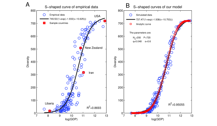
Figure 1: The S-shaped relationship between log(GDP) ($X_{i}$) and the export diversity $D_{i}$ of countries. (A) The original data and the logistic fitting for all countries in 1995. (B) The blue scatter points are the simulation results from our tri-partite model. Whereas the red curve is the analytic result of Equation 11(see section II.2 of main text), the black curve is the logistic fitting.

From FIG.1, we observe that all countries can be divided into three groups: small countries that are in the lower part of the ``S'' curve (e.g., Liberia), intermediate countries (e.g., Iran and New Zealand) that are in the ``accelerate'' part of the curve and large countries (e.g., the USA) that are at the top of the curve. The small countries in the first group can export very few varieties of goods if their sizes do not exceed a certain threshold (the ``quiescence trap''Hausmann et al. (2010)). The second segment of the ``S'' curve represents an exponential increase, in which, countries have very different types of export products. However, the accelerating-growth effect stops at the uppermost part of the ``S'' curve due to the ceiling effect of diversity, as large countries' diversification levels are not as high as an exponential curve would indicate. This pattern in the relationship between economic size and export diversity is very stable in all of the years of our data set (see Hu et al. (2011)).

II.2 Model

It is important to consider why this interdependence between size and diversity in international trade exits. In paper Hidalgo and Hausmann (2009), Hidalgo et al. proposed a tri-partite network model to account for various facts regarding export diversity and product ubiquity. In their model, the first and third layered nodes are the countries and their products, respectively, whereas the nodes in the hidden layer between countries and products are introduced to represent non-tradable elements, factors or capabilities, e.g., management skills, raw materials, regulation, property rights, etc. Thus, countries need to have these elements locally available to produce goods.

Following Hidalgo's model, we hope to account for the S-shaped relationship by constructing a modified model which also assumes that each product requires some non-trade capabilities, and each country can export a product if and only if this country possesses the required capabilities.

However, we initially link the logarithmic GDP with the degrees of the nodes that represents countries because our purpose is to explain the relationship between economic size and economic diversity. That is, the number of links to country $c$ is proportional to its logarithmic GDP $X_{c}$, but these links' end-nodes are randomly selected among the capability nodes that represents a country $i$ that possesses the given capability (see FIG.2A). Furthermore, the links between capabilities and products are randomly assigned except that they are constrained by the given connection density $q$. The tri-partite network is constructed in this way.

In Hidalgo et al.'s model, country $c$ can export product $p$ if and only if the paths from $c$ to $p$ include all of the hidden nodes that connect $c$ to $p$. Thus, all of the capabilities that are devoted to producing $p$ are possessed by country $i$. However, this mechanism cannot reproduce the ``S'' curve that models the relationship between size and diversity, and as a result, we must replace this mechanism with a new rule we have designed.

We introduce one important parameter called the ``average substitutability rate'' (or ``substitutability'') $s$ to represent the proportions of the total capabilities that are required to produce product $p$ ; these capabilities can be replaced by other available capabilities. Country $c$ can export product $p$ if and only if the paths from $c$ to $p$ cover $(1-s)*100\%$ of the capabilities required by $p$ (which would imply that the hidden nodes are connected to $p$). Hence, among the requisite capabilities, only $1-s$ fractions are necessary and other $s$ fractions are substitutable in average. When the substitutability $s$ is 0, all of the capabilities are necessary, and as a result, we recover Hidalgo et al.'s model. However, when $s$ increases, more countries can export diverse products to the same extent as the largest countries. As a result, an S-shaped curve between logarithmic GDP and diversity is obtained.

For example (see FIG. 2A), suppose that country C2 can only export product P2 when $s=0$ and that C2 cannot export P1 because all of the capabilities connected to P1 (namely, A1, A2, and A3) would have to be covered by the paths from C2 to P2, yet A1 is not covered. When $s$ increases to 0.5, only 50% of the capabilities must be covered by the paths. Therefore, C2 can export P1 because more than half of the capabilities required by P2 have been covered.

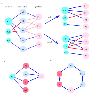
Figure 2: A concept graph of three-layer network and the analytic solution. (A) This three-layer network is designed to depict the mapping between countries and products. The nodes in the first layer represent countries and the nodes' sizes represent logarithmic their GDPs. The nodes in the second and third layers represent the capabilities and products, respectively. A country can produce more products when the substitutability $s$ increases. (B) Provided that country $c$ has L distinct capabilities (such capabilities are colored in red), the probability that this country produces product $p$ is determined by the mapping between these capabilities and product $p$. (C) The $m$ capabilities required by product $p$ can be divided into two groups based on whether they match the capabilities that are owned by country $c$.

In general, we consider N countries whose logarithmic GDPs are ($X_{1},X_{2},\cdot\cdot\cdot,X_{N}$). The adjacency matrix between countries and capabilities is $C_{ik}$, and its elements are randomly assigned:

$$C_{ik}= 1, r_{i}$$ with probability (2a)

$$C_{ik}= 0,$$ otherwise, (2b)

where the subscript $k$ is iterated from 1 to $N_{a}$ (which is the total number of capabilities we consider). To link the number of capabilities that a country has with this country's GDP, we assume that the probability $r_{i}$ is proportional to the value of $X_{i}$ of country $c_{i}$ symbolically,

$${r_{i}\propto\log(X_{i})}$$ (3)

Actually, any linear relationship between $r_{i}$ and $X_{i}$ can produce an S-shaped curve. In our model, we let $r_{i}=(X_{i}-X_{m})/(X_{M}-X_{m})$ to reduce the number of parameters as much as possible, where $X_{M}$ and $X_{m}$ are the largest and smallest value of log(GDP) in the list of countries, respectively. Additionally, we assign connections from product $p_{j}$ to the required capabilities with probability $q$. The matrix $P_{kj}$ represents the connections between these two layers:

$$P_{kj}= 1, q$$ with probability (4a)

$$P_{kj}= 0,$$ otherwise. (4b)

In the above equation, $j$ is iterated from 1 to $P$ (the total number of possible products). Suppose the adjacency matrix between countries and products is $M_{ij}$. We assume that country $c_{i}$ can export product $p_{j}$( i.e., that $M_{ij}=1$), if and only if the proportion of capabilities that are owned by the producing countries is at least a certain percent ($s$) of the total number of capabilities that are required by products:

$$M_{ij}= 1, {\sum_{k}}C_{ik}P_{kj}\geq(1-s){\sum_{k}}P_{kj}$$ if (5a)

$$M_{ij}= 0,$$ otherwise. (5b)

Finally, the export diversity $D_{i}$ is defined as the total number of types of products that country $c_{i}$ exports, namely,

$${D_{i}=}{\sum_{j}M_{ij}}.$$ (6)

In the simulations, all $X_{i}$s are defined by the real-world log(GDP) data that we have collected, the number of countries is $N$, and $P$ is defined as the total number of products in our data-set. The number of capabilities $N_{a}$, the link density between the capabilities and products $q$, and the substitutability rate $s$ are the parameters. In each simulation, we can generate a tri-partite network according to the rules we introduced, and as a result, the relationship between $X_{i}$ and $D_{i}$ can be derived.

II.3 Analytic solution

Before giving the simulation results, we will first derive the analytic relation between $D_{i}$ and $X_{i}$ to explain the mathematical essence of this model can be grasped.

In our model, all of the connections among the countries, capabilities and products are independent per se. Therefore, by analyzing the probability that a typical country $c_{i}$ exports a specific product $p_{j}$, we can derive its export diversity:

$$D_{i}=P\pi_{i}.$$ (7)

where, $\pi_{i}$ is the probability that country $c_{i}$ can produce any specific product.

Suppose the capabilities that country $c_{i}$ possesses and that product $p_{j}$ requires are $k_{c_{i}}$ and $k_{p_{j}}$, respectively. Because the density of capability that a country has is proportional to $X_{i}$, the expectation value of $k_{c_{i}}$ is also proportional to $X_{i}$. To simplify our discussion, we treat $k_{c_{i}}$ as a predetermined value and use $k_{c_{i}}$ to represent its expectation value.

The probability $\pi_{i}$ can be decomposed into various other probabilities as follows:

$$\pi_{i}={\sum_{m=0}^{N_{a}}}\Pr\{k_{p_{j}}=m\}\cdot\Pr\{c_{i}\rightarrow p_{j}|k_{p_{j}}=m\},$$ (8)

where $\Pr\{c_{i}\rightarrow p_{j}|k_{p_{j}}=m\}$ is the probability that country $c_{i}$ exports product $p_{j}$, which depends on the degree ($k_{p_{j}}$) of $p_{j}$ being $m$.

First, because a product has a probability q of requiring one capability, the number of capabilities $k_{p_{j}}$ required by $p_{j}$ satisfies a binomial distribution. Hence, we know the probability that node $p_{j}$ requires $m$ distinct capabilities is:

$$\Pr\{(k_{p_{j}}=m)\}=\binom{N_{a}}{m}q^{m}(1-q)^{N_{a}-m}.$$ (9)

Second, we derive $\Pr\{c_{i}\rightarrow p_{j}|k_{p_{j}}=m\}$. If the number of connections of nodes $c_{i}$ and $p_{j}$ are given, then the situation can be as depicted by FIG.2B. The probability $\Pr\{c_{i}\rightarrow p_{j}|k_{p_{j}}=m\}$ is the number of connection configurations satisfying that the number of elements in the set of capabilities that are connected with both $c_{i}$ and $p_{j}$ is larger than $(1-s)m$ over all of the possible connection configurations. This number is computed by means of the following steps:

i) There are $N_{a}(N_{a}-1)(N_{a}-2)\cdots(N_{a}-m+1)$(i.e., permutation $P_{N_{a}}^{m}$) ways that the product $p_{j}$ is connected to $m$ capabilities.

ii) All of the $m$ capabilities that are required by product $p_{j}$ can be divided into two groups based on whether they are owned by country $c_{i}$. Without loss of generality, suppose there are $n$ capabilities in the first group (that are possessed by $c_{j}$, i.e., $A3$ and $A4$ in FIG.2B), and $m-n$ capabilities in the second group (i.e., $A2$ in FIG.2B). (See FIG.2C.)

iii) There are $P_{k_{c_{i}}}^{n}=k_{c_{i}}(k_{c_{i}}-1)(k_{c_{i}}-2)\cdots(k_{c_{i}}-n+1)$ ways to match the capabilities in the first group.

iv) Similar to iii), the number of ways that the capabilities in the second group can be matched with the $k_{c_{i}}-n$ capabilities that are not owned by country $c_{i}$ is $P_{N_{a}-k_{c_{j}}}^{m-n}$.

v) There are $\binom{m}{n}$ ways to select $n$ elements from $m$ capabilities.

Indeed, because there must be at least $[(1-s)m]$ capabilities in the first group,so we can obtain:

$$\Pr\{c_{i}\rightarrow p_{j}|k_{p_{j}}=m\}={\sum_{n=n_{1}}^{m}}\frac{\binom{m}{n}P_{k_{c_{i}}}^{n}P_{N_{a}-k_{c_{i}}}^{m-n}}{P_{N_{a}}^{m}}.$$ (10)

In the above equation, the summation index $n$ begins at $n_{1}=\max([(1-s)m],k_{c_{i}}+m-N_{a})$ because the number of capabilities ($k_{c_{i}}-n$) that are not owned by $c_{i}$ cannot exceed $N_{a}-m$ and $n$ must be larger than $k_{c_{i}}+m-N_{a}$. By inserting Equations 10 and 9 into Equations 8 and 7, we can derive the following:

$$D_{i}=P{\sum_{m=0}^{N_{a}}}\binom{N_{a}}{m}q^{m}(1-q)^{N_{a}-m}\sum_{n=n_{1}}^{m}\frac{\binom{m}{n}P_{k_{c_{i}}}^{n}P_{N_{a}-k_{c_{i}}}^{m-n}}{P_{N_{a}}^{m}}.$$ (11)

Notice that $k_{c_{i}}\propto X_{i}$, which implies that $D_{i}$ is actually a function of $X_{i}$.

Although Equation 11 accurately models the relation between $X_{i}$ and $D_{i}$, it is complex; however, we can simplify it to an approximate but compact form. If we allow duplicate links to exist in the network, then the permutations in Equation 11 can be replaced by exponentials, and thus, each permutation $P_{x}^{y}$ can be replaced with $x^{y}$. Furthermore, we can use $[(1-s)m]$ to approximate $\max([(1-s)m],k_{c_{i}}+m-N_{a})$; then, we have

$$D_{i}\approx P\sum_{m=0}^{N_{a}}\binom{N_{a}}{m} q^{m}(1-q)^{N_{a}-m}\cdot$$ (12)

$$\sum_{n=[(1-s)m]}^{m}\binom{m}{n}(\frac{k_{c_{i}}}{N_{a}})^{n}(1-\frac{k_{c_{i}}}{N_{a}})^{m-n}.$$

When $s=0$, Equation 12 becomes $(\frac{k_{c_{i}}q}{N_{a}}+1-q)^{N_{a}}$ according to the binomial theorem. Because Equation 12 is the same equation as the relation between capability and diversity derived that was in paper Hausmann et al. (2010), Equation 12 is actually a general definition of $D_{i}$ in terms of $X_{i}$ in which substitutability between capabilities is allowed.

III Results

III.1 The S-shaped curve

In the previous sections we introduced our model. Here, we will give our simulation and numeric results.

In FIG.1B, the blue circles represent the simulation results and the red squares represent both the numeric results of Equation 12 and the logistic fitting. When we set the number of capabilities ($N_{a}$) at 200 Hidalgo and Hausmann (2009), the number of products ($P$) at 720 (which is also the maximum product diversity of the countries in our empirical data), the link density of capabilities and products ($q$) at 0.048, and the substitutability at 0.6, we obtain an ``S'' curve that resembles the empirical curve of best fit for the data recorded in 1995. Furthermore, we use the logistic Equation 1 to fit both the empirical and theoretical curves and to compare their fitting parameters. We found that the parameters are similar: whereas $A=749.53,k=1.932,X_{M}=10.625$ for the empirical curve, $A=737.47,k=1.938,X_{M}=10.753$ for the theoretical curve. Therefore, we conclude that our model can simulate the empirical S-shaped relationship very well.

III.2 Parameter Space

Although there are several parameters, the most important ones are $q$ and $s$. In fact, we can fix the other parameters (specifically, we select $P=720$ and $N_{a}=200$) and study how $q$ and $s$ affect the shape of the ``S'' curve. From the notions introduced above, the parameter $q$ determines the capabilities that are required by products. Thus, we can understand $q$ as the average complexity of all products. As $q$ increases, countries find it more difficult to make products, and as a result, the S-shaped curve is steeper and the diversity gap between rich countries and poor countries becomes large (see FIG.3A and Hidalgo et al. (2007); Ausloos and Lambiotte (2007)).

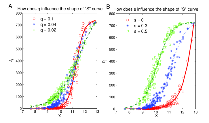
Figure 3: The S-shaped relationship, which depends on our model's parameters. (A) These S-shaped curves change if the parameter $q$ changes and the other parameters are kept fixed; when $q$ increases, the S-shaped curve becomes steeper and the trade gap among countries increases. (B) These S-shaped curves change if the parameter $s$ changes and the other parameters are kept fixed. The ceiling of the S-shaped curve emerges when $s$ increases sufficiently.

The parameter $s$ represents the average substitutability degree of the products: one country must possess a proportion of $1-s$ of the capabilities required by a product if this country wants to export that product. From FIG.3B, no ceiling for the S-shaped curve can be observed when $s$ is small because countries need to have locally almost all of the capabilities required by products in this case. Thus, when $s$ is zero, the simulation result is the same as the result of Hidalgo's model. In contrast, a ceiling for the export diversity emerges as $s$ increases because more capabilities that are required by products can be replaced by other available capabilities that are owned by producing countries. Hence, the resources (for instance, labor, skills, fund and so on) required to produce the goods in question are more diverse.

More numeric experiments are implemented to investigate how the shape of the ``S'' curve changes with changes in the combinations of $q$ and $s$. The results show that the parameter space (i.e., the combinations of $q$ and $s$) can be decomposed into several regions, as shown in FIG.4. The blue region in FIG.4 represents the combinations of $q$ and $s$ that can generate a curve that models the relationship between size and diversity and that exhibits an obvious ``S'' shape. However, the curves in every parameter region except for the blue one have the shape of twisted ``S'' curves only partially. We can distinguish these regions by considering the third- order derivatives ($d^{(3)}D_{i}/dX_{i}^{3}$): if the third-order-derivative curve $d^{(3)}D_{i}/dX_{i}^{3}$ can be separated by the x-axis into three segments, then the original curve is clearly S-shaped. However, if the curve of $d^{(3)}D_{i}/dX_{i}^{3}$ has only one or two segments that are divided by the x-axis, then the original curves are not S-shaped.

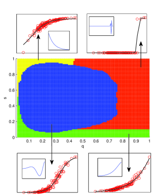
Figure 4: Different curves and their third-order derivatives in parameter space. The different regions of parameters $q$ and $s$ with different colors represent different shapes of the numeric curves in our model. Additionally, the small figures plot the curves between $X_{i}$ and $D_{i}$ and the insets show their third-order derivatives.

To quantitatively characterize the curves that model the relationship between $X_{i}$ and $D_{i}$, we use the logistic function (Equation 1) to fit the curves and show how the parameters (i.e., $k$ and $x_{m}$) change when the combinations of $q$ and $s$ are varied (FIG.5). However, we only show the regions of $q$ and $s$ that will generate a stable ``S'' shape because the logistic fitting would otherwise give unreasonable fitting parameters. From FIG.5, we can observe that whereas the slope ($k$) of $X_{i}$-$D_{i}$ is influenced mainly by $q$ and not $s$, the center position of the curve is determined mainly by $s$.

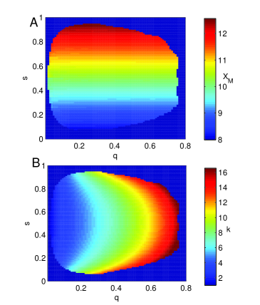
Figure 5: The parameters $X_{M}$ (A) and $k$ (B) of the logistic function depend on the parameter $q$ and $s$ in our model. Only the parameter regions that can generate ``S'' curves are shown; the blue areas are blank.

IV Discussion

In general, this paper discusses how the revision of Hidalgo et al.'s tri-partite network model can generate the observed S-shaped curve of the global export diversity, which depends on the economic sizes of countries. In this model, we found that the substitutability $s$ is an important parameter that can account for the ceiling effect in the S-shaped curve. When $s$ decreases, the size - diversity curve increasingly resembles a logistic curve and becomes dissimilar to the exponential function predicted by paper Hausmann et al. (2010). Therefore, we claimed the substitutability between different capabilities cannot be ignored because the empirical size - diversity curve has an S-shape.

However, this work is only the first step toward a fuller understanding of the export diversity in international trade. The S-shaped curve that models the relationship between diversity and economic size can only show the aggregate information regarding one country's export diversity. Additional studies that investigate the distribution of different products in a given country are worth conducting in future.