Averaging operators over homogeneous varieties over finite fields

Abstract.

In this paper we study the mapping properties of the averaging operator over a variety given by a system of homogeneous equations over a finite field. We obtain optimal results on the averaging problems over two dimensional varieties whose elements are common solutions of diagonal homogeneous equations. The proof is based on a careful study of algebraic and geometric properties of such varieties. In particular, we show that they are not contained in any hyperplane and are complete intersections. We also address partial results on averaging problems over arbitrary dimensional homogeneous varieties which are smooth away from the origin.

1. Introduction

1.1. Motivation

Analysis in finite fields is a useful subject because it interacts with other mathematical fields. In addition, the finite field case serves as a typical model for the Euclidean case and possesses structural advantages which enable us to relate our problems to other well-studied problems in number theory, arithmetic combinatorics, or algebraic geometry. For these reasons, problems in Euclidean harmonic analysis have been recently reformulated and studied in the finite field setting. For example, see [3, 4, 5, 9, 15, 18, 23] and references therein. In this paper we investigate $L^{p}-L^{r}$ estimates of averaging operators over algebraic varieties given by a system of homogeneous polynomials in finite fields. For Euclidean averaging problems, we refer readers to [10] and [16]. We begin with notation and definitions for averaging problems in finite fields. Let $\mathbb{F}_{q}^{d}$ be a $d$-dimensional vector space over a finite field $\mathbb{F}_{q}$ with $q$ elements. Throughout this paper, we assume that the characteristic of $\mathbb{F}_{q}$ is sufficiently large. We denote by $dm$ the counting measure on the space $\mathbb{F}_{q}^{d}$. The pair $(\mathbb{F}_{q}^{d},dm)$ is named as a function space. We now consider a frequency space, denoted by the pair $(\mathbb{F}_{q^{*}}^{d},dx)$, where $\mathbb{F}_{q^{*}}^{d}$ and $dx$ denote the dual space of $\mathbb{F}_{q}^{d}$ and the normalized counting measure on $\mathbb{F}_{q^{*}}^{d}$, respectively. Since $\mathbb{F}_{q}^{d}$ is isomorphic to $\mathbb{F}_{q^{*}}^{d}$ as an abstract group, we identify $\mathbb{F}_{q}^{d}$ with $\mathbb{F}_{q*}^{d}$. For instance, we write $(\mathbb{F}_{q}^{d},dx)$ for $(\mathbb{F}_{q^{*}}^{d},dx)$. This convention helps us to avoid complicated notation appearing in doing some computations. We shorten both $(\mathbb{F}_{q}^{d},dm)$ and $(\mathbb{F}_{q}^{d},dx)$ as just $\mathbb{F}_{q}^{d}$ if there is no risk of confusion between the function space $(\mathbb{F}_{q}^{d},dm)$ and the frequency space $(\mathbb{F}_{q}^{d},dx)$. Let $V$ be an algebraic variety in the frequency space $(\mathbb{F}_{q}^{d},dx)$. We endow $V$ with a normalized surface measure, denoted by $d\sigma$, which can be defined by the relation

$$\int f(x)~{}d\sigma(x)=\frac{1}{|V|}\sum_{x\in V}f(x),$$

where $f:(\mathbb{F}_{q}^{d},dx)\to\mathbb{C}$ and $|V|$ denotes the cardinality of $V$. Notice that we can replace $d\sigma(x)$ by $q^{d}|V|^{-1}V(x)dx$, where $V(x)$ indicates the characteristic function on $V$. Then the convolution function of $f$ and $d\sigma$ is defined on $(\mathbb{F}_{q}^{d},dx)$:

$$f\ast d\sigma(y)=\int_{\mathbb{F}_{q}^{d}}f(y-x)~{}d\sigma(x)=\frac{1}{|V|}\sum_{x\in V}f(y-x).$$

In the finite field setting, the averaging problem is to determine $1\leq p,r\leq\infty$ such that

(1.1) $$\|f\ast d\sigma\|_{L^{r}(\mathbb{F}_{q}^{d},dx)}\leq C\|f\|_{L^{p}(\mathbb{F}_{q}^{d},dx)}\quad\text{for all}~{}~{}f:\mathbb{F}_{q}^{d}\to\mathbb{C},$$

where $C>0$ is independent of the function $f$ and the size of the underlying finite field.

Definition 1.1.

We use $\mathfrak{P}(p,r)$ to indicate that inequality (1.1) holds.

As an analogue of averaging problems in Euclidean space, this problem has first been addressed by Carbery, Stones and Wright [3]. They mainly investigated the $L^{p}-L^{r}$ estimates of the averaging operator over a $k$-dimensional variety given by a vector-valued polynomial $P_{k}:\mathbb{F}_{q}^{k}\to\mathbb{F}_{q}^{d}$. In particular, Carbery, Stones, and Wright [3] consider a variety ${\mathcal{V}}_{k}\subseteq\mathbb{F}_{q}^{d},1\leq k\leq d-1$, which is given by the range of $P_{k}:\mathbb{F}_{q}^{k}\to\mathbb{F}_{q}^{d}$ defined by

$$P_{k}(t)=\left(t_{1},t_{2},\ldots,t_{k},t_{1}^{2}+t_{2}^{2}+\cdots+t_{k}^{2},\ldots,t_{1}^{d-k+1}+\cdots+t_{k}^{d-k+1}\right)$$

for

$$t=(t_{1},t_{2},\ldots,t_{k})\in\mathbb{F}_{q}^{k}.$$

Observe that the generalized parabolic variety ${\mathcal{V}}_{k}$ can be written by

(1.2) $${\mathcal{V}}_{k}=\{x\in\mathbb{F}_{q}^{d}:g_{1}(x)=g_{2}(x)=\cdots=g_{d-k}(x)=0\},$$

where $g_{j}(x)=x_{1}^{j+1}+x_{2}^{j+1}+\cdots+x_{k}^{j+1}-x_{k+j}$ for $j=1,2,\ldots,d-k$. Namely, the variety ${\mathcal{V}}_{k}$ is exactly the collection of the common solutions of the $d-k$ equations: $g_{j}(x)=0$ for $j=1,2,\ldots,d-k$. It is clear that $|{\mathcal{V}}_{k}|=q^{k}$ for all $k=1,2,\ldots,d-1$, because $x_{k+1},\ldots,x_{d}\in\mathbb{F}_{q}$ are uniquely determined whenever we choose $x_{1},x_{2},\ldots,x_{k}\in\mathbb{F}_{q}$. Applying the Weil theorem [22], the aforementioned authors [3] have obtained the sharp Fourier decay estimates on the variety ${\mathcal{V}}_{k}$ and, as a consequence, they give the complete solution of the averaging problem over the variety ${\mathcal{V}}_{k}$. Before we present the result of [3], we need to introduce one more notation:

Definition 1.2.

For points $P_{1},\ldots,P_{s}\in\mathbb{R}^{2}$ of the Euclidean plane, we use $\left\langle P_{1},\ldots,P_{s}\right\rangle$ to denote their convex hull.

We use Definitions 1.1 and 1.2 to formulate our main results, in which $\mathfrak{P}(p,r)$ is related to belonging the point $(1/p,1/r)$ to certain convex polygon.

We also denote

$$P_{0,0}=(0,0),\qquad P_{0,1}=(0,1),\qquad P_{1,1}=(1,1).$$

It is shown in [3] that

(1.3) $$\mathfrak{P}(p,r)\iff\left(\frac{1}{p},\frac{1}{r}\right)\in\left\langle P_{0,0},P_{0,1},P_{1,1},\left(\frac{d}{2d-k},\frac{d-k}{2d-k}\right)\right\rangle.$$

However, if the variety ${\mathcal{V}}_{k}$ is replaced by the homogeneous variety ${\mathcal{H}}_{k}$ defined as

(1.4) $${\mathcal{H}}_{k}=\{x\in\mathbb{F}_{q}^{d}:h_{1}(x)=h_{2}(x)=\cdots=h_{d-k}(x)=0\},$$

where $h_{j}(x)=x_{1}^{j+1}+x_{2}^{j+1}+\cdots+x_{k}^{j+1}-x_{k+j}^{j+1}$ for $j=1,2,\ldots,d-k$, then the averaging problem over ${\mathcal{H}}_{k}$ becomes much harder. There are two main reasons why it is difficult to find sharp $L^{p}-L^{r}$ averaging estimates over ${\mathcal{H}}_{k}$. First, it is not clear to find the size of ${\mathcal{H}}_{k}$. Second, the computation of the Fourier decay estimate on ${\mathcal{H}}_{k}$ is not easy, in part because it can not be obtained by simply applying the Weil theorem [22]. Moreover, it may be possible that the Fourier decay on ${\mathcal{H}}_{k}$ is slower than that on ${\mathcal{V}}_{k}$, because the homogeneous variety ${\mathcal{H}}_{k}$ contains lots of lines which could be key factors to make ${\mathcal{H}}_{k}$ flat. These reasons suggest that the $L^{p}-L^{r}$ averaging estimates over ${\mathcal{V}}_{k}$ maybe be much better than those over ${\mathcal{H}}_{k}$. In some cases, it is true but is not always true in the finite field setting. Indeed, we show here that if $k=2$, then ${\mathcal{V}}_{k}$ and ${\mathcal{H}}_{k}$ yield the same $L^{p}-L^{r}$ averaging estimates.

1.2. Conjecture on the averaging problem over ${\mathcal{H}}_{k}$

The $L^{p}-L^{r}$ averaging estimates over ${\mathcal{H}}_{k}$ depend on the maximal dimension of subspaces lying in the variety ${\mathcal{H}}_{k}$. Let us denote by $d\sigma_{k}$ the normalized surface measure on ${\mathcal{H}}_{k}$. For a moment, let us assume that $|{\mathcal{H}}_{k}|=(1+o(1))q^{k}$ for $k=2,3,\ldots,d-1$, which in fact follows from Proposition 1.9 and Lemma 3.5 below.

We recall that for any real $U$ and $V$, $U\lesssim V$ or $V\gtrsim U$ means that there exists $C>0$ independent of $q$ such that $|U|\leq CV$, and $U\asymp V$ is used to indicate that $U\lesssim V$ and $V\lesssim U$. Throughout the paper, the implied constants may depend on degrees and the number of variables of the polynomials defining algebraic varieties under consideration, in particular on the integer parameters $d,k,s$.

Suppose that the following averaging estimate over ${\mathcal{H}}_{k}$ holds true for $1\leq p,r\leq\infty$:

$$\|f\ast d\sigma_{k}\|_{L^{r}(\mathbb{F}_{q}^{d},dx)}\lesssim\|f\|_{L^{p}(\mathbb{F}_{q}^{d},dx)}\quad\text{for all}~{}~{}f:\mathbb{F}_{q}^{d}\to\mathbb{C}.$$

Then taking $f=\delta_{0}$ as a test function, it follows that

(1.5) $$\mathfrak{P}(p,r)\Longrightarrow\left(\frac{1}{p},\frac{1}{r}\right)\in\left\langle P_{0,0},P_{0,1},P_{1,1},\left(\frac{d}{2d-k},\frac{d-k}{2d-k}\right)\right\rangle,$$

where $\delta_{0}(x)=1$ if $x=(0,\ldots,0)$ and $\delta_{0}(x)=0$ otherwise. In fact, this necessary condition for $\mathfrak{P}(p,r)$ has been observed by the authors in [3] who have also remarked that if ${\mathcal{H}}_{k}$ contains an $\alpha$-dimensional subspace $\Pi_{k}$ with $\alpha>k/2$, then the necessary condition (1.5) can be improved as

(1.6) $$\mathfrak{P}(p,r)\Longrightarrow\left(\frac{1}{p},\frac{1}{r}\right)\in\left\langle P_{0,0},P_{0,1},P_{1,1},Q_{d,k,\alpha},R_{d,k,\alpha}\right\rangle,$$

where

$$\begin{split}Q_{d,k,\alpha}&=\left(\frac{k^{2}+\alpha d-2\alpha k}{k(d-\alpha)},\frac{\alpha(d-k)}{k(d-\alpha)}\right),\\ R_{d,k,\alpha}&=\left(\frac{d(k-\alpha)}{k(d-\alpha)},\frac{(d-k)(k-\alpha)}{k(d-\alpha)}\right).\end{split}$$

Hence, to find a more precise necessary condition for $\mathfrak{P}(p,r)$, we need to observe the maximal dimension $\alpha$ of the subspaces $\Pi_{k}$ lying in the homogeneous variety ${\mathcal{H}}_{k}$. Since $\alpha$ is always an integer, if $k$ is odd, then it is impossible that ${\mathcal{H}}_{k}$ contains a $k/2$-dimensional subspace $\Pi_{k}$. In this case, if $-1\in\mathbb{F}_{q}$ is a square number, then it may happen that $|\Pi_{k}|=q^{(k+1)/2}$ (namely $\alpha=(k+1)/2$). However, if $k$ is even, then $\alpha$ can be taken as an integer $k/2$. Combining these observations with (1.5) and (1.6), we are lead to the following conjecture (see Figure 1.1).

Conjecture 1.3.

For each $k=2,3,\ldots,d-1$, let ${\mathcal{H}}_{k}$ be the homogeneous variety defined as (1.4).

• If $k$ is even, we have

  $$\mathfrak{P}(p,r)\iff\left(\frac{1}{p},\frac{1}{r}\right)\in\left\langle P_{0,0},P_{0,1},P_{1,1},\left(\frac{d}{2d-k},\frac{d-k}{2d-k}\right)\right\rangle.$$

• If $k$ is odd and $-1\in\mathbb{F}_{q}$ is a square, then

  $$\mathfrak{P}(p,r)\iff\left(\frac{1}{p},\frac{1}{r}\right)\in\left\langle P_{0,0},P_{0,1},P_{1,1},S_{d,k},T_{d,k}\right\rangle,$$

  where

  $$\begin{split}S_{d,k}&=\left(\frac{dk-2k+d}{k(2d-k-1)},\frac{(k+1)(d-k)}{k(2d-k-1)}\right),\\ T_{d,k}&=\left(\frac{d(k-1)}{k(2d-k-1)},\frac{(d-k)(k-1)}{k(2d-k-1)}\right).\end{split}$$

When $d\geq 3$ is odd and $k=d-1$, it is observed in [14] that the conjecture holds true. In the case when $d\geq 4$ is even and $k=d-1$, the conjecture has recently been established in [13]. Namely, the averaging problem over $H_{d-1}$ has been completely solved where $H_{d-1}=\{x\in\mathbb{F}_{q}^{d}:x_{1}^{2}+x_{2}^{2}+\ldots+x_{d-1}^{2}-x_{d}^{2}=0\}$ and $-1\in\mathbb{F}_{q}$ is a square. However, there are no known results on the conjecture for $k=2,3,\ldots,d-2$.

1.3. Statement of main results

Our first result below says that Conjecture 1.3 is true for any integer $d\geq 3$ and $k=2$ (see Figure 1.1).

For each $k=2,3,\ldots,d-1$, let $d\sigma_{k}$ be the normalized surface measure on the homogeneous variety ${\mathcal{H}}_{k}\subseteq\mathbb{F}_{q}^{d}$ given in (1.4).

Theorem 1.4.

If $d\geq 3$ is an integer and $k=2$, then, assuming that the characteristic of $\mathbb{F}_{q}$ is sufficiently large,

$$\mathfrak{P}(p,r)\iff\left(\frac{1}{p},\frac{1}{r}\right)\in\left\langle P_{0,0},P_{0,1},P_{1,1},\left(\frac{d}{2d-2},\frac{d-2}{2d-2}\right)\right\rangle.$$

Remark 1.5.

As mentioned before, this statement has only been known in [14] for $d=3$ and $k=2$. Notice from Theorem 1.4 that the optimal averaging result for the homogeneous variety ${\mathcal{H}}_{2}$ is exactly the same as that in (1.3) for the general parabolic variety ${\mathcal{V}}_{2}$ defined in (1.2).

Let $\mathbb{A}^{d}$ be the affine $d$-space $\overline{\mathbb{F}}_{q}^{d}$, where $\overline{\mathbb{F}}_{q}$ denotes the algebraic closure of the finite filed $\mathbb{F}_{q}$ with $q$ elements.

For each $k=2,3,\ldots,d-1$, let us consider the algebraic variety

$$\overline{{\mathcal{H}}}_{k}=\{x\in\mathbb{A}^{d}:h_{1}(x)=h_{2}(x)=\ldots=h_{d-k}(x)=0\},$$

where $h_{j}$, $j=1,\ldots,d-k$, are the homogeneous polynomials defined as in (1.4). One interesting point is that the smoothness of $\overline{{\mathcal{H}}}_{k}$ depends on the dimension $d$ of $\mathbb{A}^{d}$. Indeed, we see from Proposition 1.10 below that the variety $\overline{{\mathcal{H}}}_{k}$ is smooth away from the origin if and only if $d-k=1,2,3$. In the case when $\overline{{\mathcal{H}}}_{k}$ for $k\geq 3$ is smooth away from the origin, we are able to obtain certain $L^{p}-L^{r}$ averaging estimates on ${\mathcal{H}}_{k}$ (see Figure 1.1).

Next, we state our averaging results over ${\mathcal{H}}_{k}$ for $k\geq 3$.

Theorem 1.6.

If $\max\{d-3,3\}\leq k\leq d-1$, then, assuming that the characteristic of $\mathbb{F}_{q}$ is sufficiently large,

$$\left(\frac{1}{p},\frac{1}{r}\right)\in\left\langle P_{0,0},P_{0,1},P_{1,1},\left(\frac{d-1}{2d-k-1},\frac{d-k}{2d-k-1}\right)\right\rangle\Longrightarrow\mathfrak{P}(p,r).$$

Remark 1.7.

The result of Theorem 1.6 is far from the conjectured averaging result, but in general it gives a sharp $L^{p}-L^{r}$ estimate for $p=(2d-k-1)/(d-1)$.

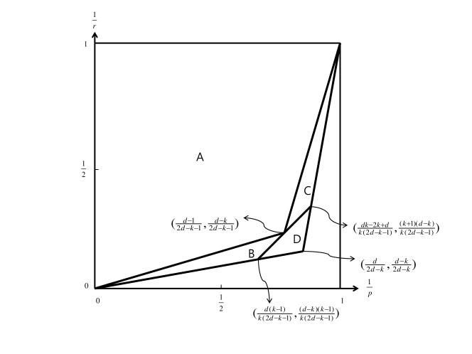
Figure 1.1. When $k\geq 2$ is even, $A\cup B\cup C\cup D$ is region of $(1/p,1/r)$ of Conjecture 1.3. Theorem 1.4 covers the conjectured region for $k=2$. Furthermore, $A\cup B\cup C$ indicates the conjectured region in the case when $k\geq 3$ is odd and $-1\in\mathbb{F}_{q}$ is a square number. The region $A$ is corresponding to the result of Theorem 1.6.

Our work has been mainly motivated by the exponential sum estimates on abstractly given homogeneous varieties due to authors in [19]. To prove our main results, we first derive a useful result about averaging on general homogeneous varieties with abstract algebraic structures. Then our main results follow by applying it to our variety ${\mathcal{H}}_{k}$. To do this, we make the following three key observations on ${\mathcal{H}}_{k}\subseteq\mathbb{F}_{q}^{d}$ for $k=2,3,\ldots,d-1$.

Proposition 1.8.

Suppose that the characteristic of $\mathbb{F}_{q}$ is sufficiently large. Then, for every $k=2,\ldots,d-1$, the algebraic variety $\overline{{\mathcal{H}}}_{k}\subseteq\mathbb{A}^{d}$ is not contained in any hyperplane in $\mathbb{A}^{d}$.

Proposition 1.9.

Suppose that the characteristic of $\mathbb{F}_{q}$ is sufficiently large. Then for every $k=2,\ldots,d-1$, the algebraic variety $\overline{{\mathcal{H}}}_{k}\subseteq\mathbb{A}^{d}$ is absolutely irreducible and $\dim\overline{{\mathcal{H}}}_{k}=k$.

That is, Propositions 1.8 and 1.9 assert that ${\mathcal{H}}_{k}$ is a complete intersection.

Proposition 1.10.

Suppose that the characteristic of $\mathbb{F}_{q}$ is sufficiently large. Then for every $k=2,\ldots,d-1$, the algebraic variety $\overline{{\mathcal{H}}}_{k}\subseteq\mathbb{A}^{d}$ is smooth away from the origin if and only if $d-k=1,2,3$.

Furthermore, the smoothness condition on ${\mathcal{H}}_{2}$ is not necessary in completing the proof of Theorem 1.4. Therefore, the conclusion of Theorem 1.4 holds true for any $d$ and $k=2$, and Conjecture 1.3 for $k=2$ is established. On the contrary, we use the smooth condition on ${\mathcal{H}}_{k}$ for $k\geq 3$ in proving Theorem 1.6. Thus, the condition that $d-k=1,2,3$ is imposed to the statement of Theorem 1.6. However, Conjecture 1.3 proposes that such a smooth condition on ${\mathcal{H}}_{k}$ may not be important in determining $L^{p}-L^{r}$ averaging estimates over ${\mathcal{H}}_{k}$. We hope that experts in both harmonic analysis and algebraic geometry may be able to shed insight on the conjecture.

1.4. Overview of this paper

In the remaining parts of this paper, we concentrate on proving Theorem 1.4 and Theorem 1.6 which are our main results. Instead of proving directly main theorems, we derive them by means of working on more general homogeneous varieties with specific geometric structures.

To this end, in Section 2 we collect facts about the multiplicative character sums and the existence of a primitive prime divisor of a family of shifted monomials. In particular, we make use of a polynomial analogue of the Zsigmondy theorem which is due to Flatters and Ward [6].

Section 3 is devoted to setting up notation and basic concepts essential in defining abstract varieties in algebraic geometry.

In Section 4, we derive a result for averaging problems over general homogeneous varieties, where we adapt the standard analysis technique in [3] together with the results on exponential sums in [19], see Lemma 4.2 below. In fact, this result generalizes our main results related to ${\mathcal{H}}_{k}$.

In Section 5, we show that Lemma 4.2 applies to the variety ${\mathcal{H}}_{k}$ and complete the proofs of our main results, that is, Theorems 1.4 and 1.6.

We note that our main tool are bounds of exponential sums along algebraic varieties, which we interpret as results about the decay of Fourier coefficients.

2. Multiplicative character sums and roots of some polynomials

2.1. Root of shifted monomials

We need the following simple observation, which immediately follows from the Taylor formula (which applies if the characteristic is large enough).

Lemma 2.1.

For any fixed integer $s\geq 1$, if the characteristic of $\mathbb{F}_{q}$ is sufficiently large then for any $a\in\mathbb{F}_{q}^{*}$, the polynomial $t^{s}+a\in\mathbb{F}_{q}[t]$ has no multiple roots.

Lemma 2.2.

For any fixed integer $s\geq 1$, if the characteristic of $\mathbb{F}_{q}$ is sufficiently large then the polynomial $t^{s}+1\in\mathbb{F}_{q}[t]$ has at least one root which is not a root of the polynomials $t^{j}+1\in\mathbb{F}_{q}[t]$, $j=1,\ldots,s-1$.

Proof.

By a result of Flatters and Ward [6, Theorem 2.6], if the characteristic of $\mathbb{F}_{q}$ is large enough then $t^{2s}-1$ has an irreducible factor $q(t)\in\mathbb{F}_{q}[t]$ that does not divide any of the polynomials $t^{j}-1\in\mathbb{F}_{q}[t]$, $j=1,\ldots,2s-1$. In particular, $q(t)$ is relatively prime with $t^{s}-1$ and thus is a divisor of

$$t^{s}+1=\frac{t^{2s}-1}{t^{s}-1}.$$

Furthermore, $q(t)$ is relatively prime to

$$t^{j}+1=\frac{t^{2j}-1}{t^{j}-1},\qquad j=1,\ldots,s-1,$$

which concludes the proof. ∎

2.2. Multiplicative character sums with shifted monomials

We also need the following result due to Wan [21, Corollary 2.3] that follows almost instantly from the Weil bound in the form given in [11, Theorem 11.23].

Lemma 2.3.

Let $g_{1}(t),\ldots,g_{s}(t)$ be $s$ monic pairwise prime polynomials in $\mathbb{F}_{q}[t]$. Denote by $\chi_{1},\ldots,\chi_{s}$ nontrivial multiplicative characters of $\mathbb{F}_{q}$ with order $d_{1},\ldots,d_{s}$, respectively. If for some $i=1,2,\ldots,s$, the polynomial $g_{i}(t)$ is not of the form $q(t)^{d_{i}}$ with $q(t)\in\mathbb{F}_{q}[t]$, then we have

$$\left|\sum_{t\in\mathbb{F}_{q}}\chi_{1}(g_{1}(t))\cdots\chi_{s}(g_{s}(t))\right|\lesssim q^{\frac{1}{2}}.$$

Lemma 2.4.

For any fixed integer $s\geq 1$, if the characteristic of $\mathbb{F}_{q}$ is sufficiently large, then for any multiplicative characters $\chi_{j}$, $j=1,2,\ldots,s$, among which at least one is nontrivial, we have

$$\left|\sum_{t\in\mathbb{F}_{q}}\prod_{j=1}^{s}\chi_{j}(t^{j+1}+1)\right|\lesssim q^{\frac{1}{2}}.$$

Proof.

After ignoring all trivial characters, it suffices to prove that for some positive integer $m\leq s$, we have

(2.1) $$\left|\sum_{t\in\mathbb{F}_{q}}\widetilde{\chi}_{1}(t^{s_{1}+1}+1)\cdots\widetilde{\chi}_{m}(t^{s_{m}+1}+1)\right|\lesssim q^{\frac{1}{2}},$$

where $1\leq s_{1}<s_{2}<\ldots<s_{m}\leq s$ and $\tilde{\chi}_{1},\ldots,\tilde{\chi}_{m}$ denote nontrivial multiplicative characters of $\mathbb{F}_{q}$. Factoring the polynomials $t^{s_{i}+1}+1$, $i=1,\ldots,m$, into irreducible factors over $\mathbb{F}_{q}$ and using the multiplicativity, we see from Lemma  2.1 that

$$\sum_{t\in\mathbb{F}_{q}}\widetilde{\chi}_{1}(t^{s_{1}+1}+1)\cdots\widetilde{\chi}_{m}(t^{s_{m}+1}+1)=\sum_{t\in\mathbb{F}_{q}}{\eta}_{1}\left(q_{1}(t)\right)\cdots{\eta}_{u}(q_{u}(t))$$

for some multiplicative characters $\eta_{i}$ and monic pairwise prime polynomials $q_{i}$, $i=1,2,\ldots,u$.

Furthermore, by Lemma 2.2 we have $\eta_{i_{0}}=\widetilde{\chi}_{i_{0}}$ for at least one $i_{0}\in\{1,\ldots,u\}$, and thus $\eta_{i_{0}}$ is a nontrivial character. Now using Lemma 2.3 we complete the proof. ∎

3. Algebraic properties of general homogeneous varieties

3.1. Preliminaries

In this section, we review known facts on general varieties generated by a system of $s-$homogeneous polynomials in $\mathbb{F}_{q}[x_{1},x_{2},\ldots,x_{d}]$. We begin by setting up notation.

Let $2\leq s\leq d-1$ be an integer. Assume we are given $s-$homogeneous polynomials in $d$ variables over $\mathbb{F}_{q}$ of degree at least two each, which we write as

$$f_{j}(x)\in\mathbb{F}_{q}[x_{1},x_{2},\ldots,x_{d}],\quad\deg f_{j}\geq 2,\qquad j=1,\ldots,s,$$

where $x=(x_{1},x_{2},\ldots,x_{d})$. Now, define the closed algebraic set

(3.1) $$\overline{H}_{\mathbb{A}}=\{x\in\mathbb{A}^{d}~{}:~{}f_{1}(x)=f_{2}(x)=\ldots=f_{s}(x)=0\}.$$

Let $H_{\mathbb{A}}$ be the collection of points in $\overline{H}_{\mathbb{A}}$ with coordinates in $\mathbb{F}_{q}:$

(3.2) $$H_{\mathbb{A}}=\{x\in\mathbb{F}_{q}^{d}~{}:~{}f_{1}(x)=f_{2}(x)=\ldots=f_{s}(x)=0\}.$$

We also use the standard notation $\mathbb{P}^{d-1}$ for the $(d-1)$-dimensional projective space over $\overline{\mathbb{F}}_{q}$, which can be considered as the collection of all one dimensional subspaces of the vector space $\mathbb{A}^{d}$. For $P=[a_{1}:a_{2}:\ldots:a_{d}]\in\mathbb{P}^{d-1}$ and a polynomial $f\in\overline{\mathbb{F}}_{q}[x_{1},\ldots,x_{d}]$, recall that $f(P)=0$ means that $f(\lambda a_{1},\ldots,\lambda a_{d})=0$ for all $\lambda\neq 0$. Like the algebraic subset $\overline{H}_{\mathbb{A}}$ of the affine space $\mathbb{A}^{d}$, we define the projective algebraic set

$$\overline{H}_{\mathbb{P}}=\{P\in\mathbb{P}^{d-1}~{}:~{}f_{1}(P)=f_{2}(P)=\ldots=f_{s}(P)=0\}.$$

Let us recall an affine cone over a projective subset in $\mathbb{P}^{d-1}$. Denote by $\pi:\mathbb{A}^{d}\setminus\{(0,\ldots,0)\}\to\mathbb{P}^{d-1}$ the projection map defined by

$$\pi(x_{1},\ldots,x_{d})=[x_{1}:\cdots:x_{d}].$$

Then the affine cone over $Y\subseteq\mathbb{P}^{d-1}$ is defined by

$$C(Y)=\pi^{-1}(Y)\cup\{(0,\ldots,0)\}\subseteq\mathbb{A}^{d}.$$

Notice that $\overline{H}_{\mathbb{A}}$ is the affine cone over the projective variety $\overline{H}_{\mathbb{P}}$.

Definition 3.1.

We say that a homogeneous variety $H_{\mathbb{A}}\subseteq\mathbb{F}_{q}^{d}$ defined as in (3.2) is a complete intersection if the following two conditions hold:

• $\overline{H}_{\mathbb{A}}\subseteq\mathbb{A}^{d}$ is an affine cone over a projective variety $\overline{H}_{\mathbb{P}}$ which is not contained in a hyperplane,

• $\overline{H}_{\mathbb{A}}$ is an absolutely irreducible variety of dimension $d-s$ (or $\dim\overline{H}_{\mathbb{P}}=d-1-s$).

Definition 3.2.

We say that a homogeneous variety $H_{\mathbb{A}}\subseteq\mathbb{F}_{q}^{d}$ defined as in (3.2) is smooth if $\overline{H}_{\mathbb{A}}$ is smooth away from the origin.

3.2. Exponential sums and Fourier coefficients

It is observed in [19] that if $H_{\mathbb{A}}$ is a smooth homogeneous variety, which is a complete intersection, then $\overline{H}_{\mathbb{A}}\cap\overline{\Pi}(m)$ can have at most isolated singularities in $\mathbb{P}^{d-1}$ where

$$\overline{\Pi}(m)=\{x\in\mathbb{A}^{d}:m\cdot x=0\}$$

for $m\neq(0,\ldots,0)$, where $m\cdot x$ denotes the inner products of the vectors $m$ and $x$.

From this observation, they state and prove the following exponential sum estimates on $H_{\mathbb{A}}$ (see [19, Theorem 1]).

Lemma 3.3.

Let $H_{\mathbb{A}}\subseteq\mathbb{F}_{q}^{d}$ be defined as in (3.2). Suppose that $H_{\mathbb{A}}$ is a smooth homogeneous variety, which is a complete intersection, and the characteristic of $\mathbb{F}_{q}$ is sufficiently large. Then we have for all $m\in\mathbb{F}_{q}^{d}\setminus\{(0,\ldots,0)\}$

$$\left|\sum_{x\in H_{\mathbb{A}}}\psi(m\cdot x)\right|\lesssim\left\{\begin{array}[]{ll}q^{(d-s+1)/2}&\text{if}~{}~{}d-s\geq 3,\\ q&\text{if}~{}~{}d-s=2,\end{array}\right.$$

where $\psi$ denotes a nontrivial additive character of $\mathbb{F}_{q}$.

Here, we point out that the proof of Lemma 3.3 for $d-s=2$ was given by the authors in [19] without using the smoothness assumption on $H_{\mathbb{A}}$. Therefore, the smoothness condition on $H_{\mathbb{A}}$ can be relaxed for $d-s=2$. Indeed, the following bound follows immediately from a result of Cochrane [2, Theorem 4.3.5].

Lemma 3.4.

If $H_{\mathbb{A}}\subseteq\mathbb{F}_{q}^{d}$ is a homogeneous variety which is a complete intersection given by (3.2) of dimension $\dim\overline{H}_{\mathbb{A}}=d-s$, where $\overline{H}_{\mathbb{A}}$ is given by (3.1), then

$$\left|\sum_{x\in H_{\mathbb{A}}}\psi(m\cdot x)\right|\lesssim q^{d-s-1}$$

for all $m\in\mathbb{F}_{q}^{d}\setminus\{(0,\ldots,0)\}$.

The following estimate on the cardinality of $H_{\mathbb{A}}$ due to Chatzidakis, van den Dries and Macintyre [1, Proposition 3.3] gives an extension of the result of Lang and Weil [17].

Lemma 3.5.

Suppose that $\overline{V}\subseteq\mathbb{A}^{d}$ is an algebraic variety with $\nu$ absolutely irreducible components and of dimension $e$ defined by polynomials over $\mathbb{F}_{q}$ and let $V=\{x\in\overline{V}\cap\mathbb{F}_{q}^{d}\}$. Then

$$|V|-\nu q^{e}\lesssim q^{e-1/2}.$$

It is clear from Lemma 3.5 that $|H_{\mathbb{A}}|=(1+o(1))q^{d-s}$ if $H_{\mathbb{A}}$ is a homogeneous variety, given by (3.2) which is a complete intersection in $\mathbb{F}_{q}^{d}$.

Now, we endow a homogeneous variety $H_{\mathbb{A}}$ with the normalized surface measure $d\sigma_{H}$. Recall that if $f:(\mathbb{F}_{q}^{d},dx)\to\mathbb{C}$, then

$$\int f(x)~{}d\sigma_{H}(x)=\frac{1}{|H_{\mathbb{A}}|}\sum_{x\in H_{\mathbb{A}}}f(x).$$

The following decay estimates of the Fourier coefficients

$$(d\sigma_{H})^{\vee}(m)=\frac{1}{|H_{\mathbb{A}}|}\sum_{x\in H_{\mathbb{A}}}\psi(m\cdot x),\qquad m\in\mathbb{F}_{q}^{d},$$

on $H_{\mathbb{A}}$ follow immediately from Lemma 3.4 and 3.3.

Lemma 3.6.

Let $d\sigma_{H}$ be the normalized surface measure on the homogeneous variety $H_{\mathbb{A}}\subseteq\mathbb{F}_{q}^{d}$ given by (3.2), which is a complete intersection. If the characteristic of $\mathbb{F}_{q}$ is sufficiently large, then:

• If $d-s=2$, then we have

  $$|(d\sigma_{H})^{\vee}(m)|\lesssim q^{-1}$$

  for all $m\in\mathbb{F}_{q}^{d}\setminus\{(0,\ldots,0)\}$.

• If $H_{\mathbb{A}}$ is smooth and $d-s\geq 3$, then

  $$|(d\sigma_{H})^{\vee}(m)|\lesssim q^{-(d-s-1)/2}$$

  for all $m\in\mathbb{F}_{q}^{d}\setminus\{(0,\ldots,0)\}$.

4. Fourier coefficients and $L^{p}-L^{r}$ averaging estimates over $H_{\mathbb{A}}$

4.1. Estimates for varieties with given rate of decay of Fourier coefficients

First we need the following general result which can be obtained by adapting the arguments in [3]. For the sake of completeness, we provide the proof in full detail.

Lemma 4.1.

Let $d\sigma_{H}$ be the normalized surface measure on an affine homogeneous variety $H_{\mathbb{A}}\subseteq\mathbb{F}_{q}^{d}$ given by (3.2), which is a complete intersection. If $(d\sigma)^{\vee}(m)\lesssim q^{-\vartheta/2}$ for all $m\in\mathbb{F}_{q}^{d}\setminus\{(0,\ldots,0)\}$ and for some fixed $\vartheta>0$, then $\mathfrak{P}(p,r)$ holds with

$$p=\frac{2s+\vartheta}{s+\vartheta}\qquad\text{and}\qquad r=\frac{2s+\vartheta}{s}.$$

Proof.

We must show that

$$\|f\ast d\sigma_{H}\|_{L^{r}({\mathbb{F}_{q}^{d}},dx)}\lesssim\|f\|_{{L^{p}}({\mathbb{F}_{q}^{d}},dx)}$$

for all function $f:(\mathbb{F}_{q}^{d},dx)\to\mathbb{C}$ with the above values of $p$ and $r$.

Define a function $K$ on $({\mathbb{F}_{q}^{d}},dm)$ by $K=(d\sigma_{H})^{\vee}-\delta_{0}$. Observe that $d\sigma_{H}(x)=\widehat{K}(x)+\widehat{\delta_{0}}(x)=\widehat{K}(x)+1$ for $x\in(\mathbb{F}_{q}^{d},dx)$, where for a function $F$ on $({\mathbb{F}_{q}^{d}},dm)$ we define

$$\widehat{F}(x)=\sum_{m\in\mathbb{F}_{q}^{d}}F(m)\psi(-m\cdot x).$$

and, as before, $m\cdot x$ denotes the inner products of $m$ and $x$. Since $\vartheta>0$ and $dx$ is the normalized counting measure on $\mathbb{F}_{q}^{d}$, it follows from Young’s inequality (see [8, 12]) that

$$\|f\ast 1\|_{L^{r}({\mathbb{F}_{q}^{d}},dx)}\lesssim\|f\|_{L^{p}({\mathbb{F}_{q}^{d}},dx)}.$$

Thus, it suffices to prove that

(4.1) $$\|f\ast\widehat{K}\|_{L^{r}({\mathbb{F}_{q}^{d}},dx)}\lesssim\|f\|_{L^{p}({\mathbb{F}_{q}^{d}},dx)}$$

for all functions $f:(\mathbb{F}_{q}^{d},dx)\to\mathbb{C}$.

Notice that (4.1) can be obtained by interpolating

(4.2) $$\|f\ast\widehat{K}\|_{L^{2}({\mathbb{F}_{q}^{d}},dx)}\lesssim q^{-\vartheta/2}\|f\|_{L^{2}({\mathbb{F}_{q}^{d}},dx)}$$

and

(4.3) $$\|f\ast\widehat{K}\|_{L^{\infty}({\mathbb{F}_{q}^{d}},dx)}\lesssim q^{s}\|f\|_{L^{1}({\mathbb{F}_{q}^{d}},dx)}.$$

It remains to prove (4.2) and (4.3). By the definition of $K$ and the assumption that $(d\sigma_{H})^{\vee}(m)\lesssim q^{-\vartheta/2}$ for $m\neq(0,\ldots,0)$, we see that

$$\max\limits_{m\in\mathbb{F}_{q}^{d}}|K(m)|\lesssim q^{-\vartheta/2}.$$

Therefore, (4.2) follows by applying the Plancherel theorem (see [8, 12]):

$$\begin{split}\|f\ast\widehat{K}\|_{L^{2}({\mathbb{F}_{q}^{d}},dx)}&=\|f^{\vee}K\|_{L^{2}({\mathbb{F}_{q}^{d}},dm)}\\ &\lesssim q^{-\vartheta/2}\|f^{\vee}\|_{L^{2}({\mathbb{F}_{q}^{d}},dm)}=q^{-\vartheta/2}\|f\|_{L^{2}({\mathbb{F}_{q}^{d}},dx)}.\end{split}$$

To prove (4.3), notice that $|H_{\mathbb{A}}|=(1+o(1))q^{d-s}$, because $H_{\mathbb{A}}$ is a complete intersection. From Young’s inequality and the observation that $\|\widehat{K}\|_{L^{\infty}({\mathbb{F}_{q}^{d}},dx)}\lesssim q^{s}$, we obtain (4.3):

$$\|f\ast\widehat{K}\|_{L^{\infty}({\mathbb{F}_{q}^{d}},dx)}\leq\|\widehat{K}\|_{L^{\infty}({\mathbb{F}_{q}^{d}},dx)}\|f\|_{L^{1}({\mathbb{F}_{q}^{d}},dx)}\lesssim q^{s}\|f\|_{L^{1}({\mathbb{F}_{q}^{d}},dx)}.$$

Thus, the proof of Lemma 4.1 is complete. ∎

4.2. Main estimates

As a direct application of the Fourier decay estimates in Lemma 3.6, we can now derive averaging results related to general homogeneous variety $H_{\mathbb{A}}$, which is a complete intersection. Applying Lemma 4.1 with Lemma 3.6 yields the result below.

Lemma 4.2.

Let $d\sigma_{H}$ be the normalized surface measure on a homogeneous variety $H_{\mathbb{A}}\subseteq\mathbb{F}_{q}^{d}$, given by (3.2), which is a complete intersection. If the characteristic of $\mathbb{F}_{q}$ is sufficiently large, then:

• If $d-s=2$, then

  $$\mathfrak{P}(p,r)\iff\left(\frac{1}{p},\frac{1}{r}\right)\in\left\langle P_{0,0},P_{0,1},P_{1,1},\left(\frac{d}{2d-2},\frac{d-2}{2d-2}\right)\right\rangle.$$

• If $H_{\mathbb{A}}$ is a smooth and $d-s\geq 3$, then

  $$\left(\frac{1}{p},\frac{1}{r}\right)\in\left\langle P_{0,0},P_{0,1},P_{1,1},\left(\frac{d-1}{d+s-1},\frac{s}{d+s-1}\right)\right\rangle\Longrightarrow\mathfrak{P}(p,r).$$

Proof.

To prove (i), let us assume that $d-s=2$. Then $|H_{\mathbb{A}}|=(1+o(1))q^{d-s}=q^{2}$, because $H_{\mathbb{A}}$ is a complete intersection. Now, suppose that $\mathfrak{P}(p,r)$. In particular, we see that

$$q^{-(d+2r-2)/r}\asymp\|\delta_{0}\ast d\sigma_{H}\|_{L^{r}(\mathbb{F}_{q}^{d},dx)}\lesssim\|\delta_{0}\|_{L^{p}(\mathbb{F}_{q}^{d},dx)}=q^{-d/p}.$$

It therefore follows that

$$\frac{-d-2r+2}{r}\leq\frac{-d}{p}.$$

By duality, we also have

$$\frac{-d-2p^{*}+2}{p^{*}}\leq\frac{-d}{r^{*}},$$

where

$$p^{*}=\frac{p}{p-1}\qquad\text{and}\qquad r^{*}=\frac{r}{r-1}$$

denote the Hölder conjugates of $p$ and $r$, respectively. In conclusion,

(4.4) $$\left(\frac{1}{p},\frac{1}{r}\right)\in\left\langle P_{0,0},P_{0,1},P_{1,1},\left(\frac{d}{2d-2},\frac{d-2}{2d-2}\right)\right\rangle.$$

Conversely, we now assume that the inclusion (4.4) holds. If $1\leq r\leq p\leq\infty$, then it is clear that $\mathfrak{P}(p,r)$, because both $d\sigma_{H}$ and $({\mathbb{F}_{q}^{d}},dx)$ have total mass $1$. By the interpolation theorem, it therefore suffices to prove that

$$\mathfrak{P}\left(\frac{2d-2}{d},\frac{2d-2}{d-2}\right)$$

holds. Since $d-s=2$, applying Lemma 4.1 with Lemma 3.6 (i) yields the above property, and the the proof of Lemma 4.2 (i) is complete.

In order to prove (ii), it is enough to show that

$$\mathfrak{P}\left(\frac{d+s-1}{d-1},\frac{d+s-1}{s}\right)$$

holds. However, this follows immediately by using Lemma 4.1 together with Lemma 3.6 (ii). ∎

Remark 4.3.

Even if Lemma 4.2 provides us of powerful averaging results on general homogeneous varieties, applying it in practice may not be simple, because it contains certain abstract hypotheses.

5. Proofs of Main Results

5.1. Preliminaries

In this section, we complete the proofs of Theorem 1.4 and Theorem 1.6 which are considered as main theorems in this paper. We complete the proofs by showing that Lemma 4.2 is a general version of both Theorem 1.4 and Theorem 1.6. To do this, we begin by recalling from (1.4) that for each $k=2,3,\ldots,d-1$, our homogeneous variety ${\mathcal{H}}_{k}$ is exactly the common solutions in $\mathbb{F}_{q}^{d}$ of a system of the $(d-k)$ equations

(5.1) $$\begin{array}[]{ll}&h_{1}(x)=x_{1}^{2}+x_{2}^{2}+\cdots+x_{k}^{2}-x_{k+1}^{2}=0,\\ &\qquad\qquad\qquad\qquad\vdots\\ &h_{j}(x)=x_{1}^{j+1}+x_{2}^{j+1}+\cdots+x_{k}^{j+1}-x_{k+j}^{j+1}=0,\\ &\qquad\qquad\qquad\qquad\vdots\\ &h_{d-k}(x)=x_{1}^{d-k+1}+x_{2}^{d-k+1}+\cdots+x_{k}^{d-k+1}-x_{d}^{d-k+1}=0,\\ \end{array},$$

where $j=1,2,\ldots,(d-k)$. Let $s=d-k$ which is the number of homogeneous equations $h_{j}$ defining ${\mathcal{H}}_{k}$. Then it is clear that $\overline{{\mathcal{H}}}_{k}$ is an affine cone over its corresponding projective variety determined by $s$-homogeneous polynomials $h_{j}$. Thus, if we are able to show that the conclusions of Propositions 1.8 and 1.9 hold for $k=2$ then Theorem 1.4 follows from Lemma 4.2 (i). Furthermore, if all Propositions 1.8–1.10 hold true for $k\geq 3$, then Theorem 1.6 follows from Lemma 4.2 (ii) where the smoothness condition on $\overline{{\mathcal{H}}}_{k}$ is essential. In summary, to prove both Theorem 1.4 and Theorem 1.6, it suffices to justify Propositions 1.8–1.10.

5.2. Proof of Proposition 1.8

Since any hyperplane in $\mathbb{A}^{d}$ is a subspace with dimension $d-1$, it suffices to prove that there exists $d$ linearly independent points $\{P_{1},P_{2},\ldots,P_{d}\}\subseteq\overline{\mathcal{H}}_{k}$. Now fix $k=2,3,\ldots,(d-1)$. For each $j=1,2,\ldots,d-k$, choose a $\beta_{k+j}\in\mathbb{A}$ such that $\beta_{k+j}^{j+1}=1$ and $\beta_{k+j}\neq 1$. Since $\mathbb{A}$ is an algebraic closure and the characteristic of $\mathbb{F}_{q}$ is sufficiently large, the $\beta_{k+j}$ always exists. Denote by $I_{k\times k}$ the $k\times k$ identity matrix. We also define $1_{k\times(d-k)}$ as the $k\times(d-k)$ matrix whose all entries are $1$. Also define the following $(d-k)\times k$ matrix $C_{(d-k)\times k}$ and the $(d-k)\times(d-k)$ matrix $D_{(d-k)\times(d-k)}$:

$$\begin{split}&C_{(d-k)\times k}=\left[\begin{matrix}0&0&\cdots&0&1\\ 0&0&\cdots&0&1\\ \vdots&\vdots&\vdots&\vdots&\vdots\\ 0&0&\cdots&0&1\\ 0&0&\cdots&0&1\\ \end{matrix}\right],\\ &D_{(d-k)\times(d-k)}=\left[\begin{matrix}\beta_{k+1}&1&\cdots&1&1\\ 1&\beta_{k+2}&1&\cdots&1\\ \vdots&\vdots&\vdots&\vdots&\vdots\\ 1&\cdots&1&\beta_{d-1}&1\\ 1&1&\cdots&1&\beta_{d}\end{matrix}\right].\end{split}$$

Now consider the $d\times d$ matrix $M_{d\times d}$ defined by

$$M_{d\times d}=\left[\begin{matrix}P_{1}\\ P_{2}\\ \vdots\\ P_{d}\end{matrix}\right]=\left[\begin{matrix}I_{k\times k}&1_{k\times(d-k)}\\ C_{(d-k)\times k}&D_{(d-k)\times(d-k)}\end{matrix}\right].$$

Note that all $P_{1},P_{2},\ldots,P_{d}$ are solutions of a system of equations (5.1). Hence, it follows that $\{P_{1},P_{2},\ldots,P_{d}\}\subseteq\overline{{\mathcal{H}}}_{k}$ for any $k=2,3,\ldots,(d-1)$. Moreover, since $\beta_{k+j}-1\neq 0$ for all $j=1,2,\ldots,d-k$, it follows from simple Gauss elimination that the rank of the matrix $M_{d\times d}$ is exactly $d$, which completes the proof of Proposition 1.8.

5.3. Proof of Proposition 1.9

Recall from (5.1) that $\overline{{\mathcal{H}}}_{k}\subseteq\mathbb{A}^{d}$ is given by a system of $(d-k)$ homogeneous equations. For each $j=1,2,\ldots,d-k$, define an algebraic set

$$\overline{{\mathcal{H}}}_{k}^{j}=\{x\in\mathbb{A}^{d}~{}:~{}h_{j}(x)=0\},$$

where $h_{j}$ is defined by (5.1). By the definition of $\overline{{\mathcal{H}}}_{k}$, it follows that

(5.2) $$\overline{{\mathcal{H}}}_{k}=\bigcap_{j=1}^{d-k}\overline{{\mathcal{H}}}_{k}^{j}.$$

We need the following claim.

Lemma 5.1.

For each $n\in\{1,2,\ldots,(d-k-1)\}$, we have

$$\left(\bigcap_{j=1}^{n}\overline{{\mathcal{H}}}_{k}^{j}\right)\bigcap\overline{{\mathcal{H}}}_{k}^{n+1}\neq\emptyset$$

and there exists $\alpha\in\mathbb{A}^{d}$ such that

$$\quad\alpha\in\bigcap_{j=1}^{n}\overline{{\mathcal{H}}}_{k}^{j}\quad\text{and}\quad\alpha\notin\overline{{\mathcal{H}}}_{k}^{n+1}.$$

Proof.

The first part is trivial. For the second part of this claim, fix $n\in\{1,2,\ldots,(d-k-1)\}$ and let $l\in\overline{\mathbb{F}}_{q}$ with $l^{n+2}\neq 1$. Now, choose an $\alpha=(\alpha_{1},\alpha_{2},\ldots,\alpha_{d})\in\mathbb{A}^{d}$ whose coordinates satisfy that

$$\alpha_{j}=\left\{\begin{array}[]{ll}0&\text{if}~{}~{}j=2,3,\ldots,k,\\ l&\text{if}~{}~{}j=k+n+1,\\ 1&\text{otherwise.}\end{array}\right.$$

Then it is straightforward to check that $\alpha\in\bigcap_{j=1}^{n}\overline{{\mathcal{H}}}_{k}^{j}\quad\text{and}\quad\alpha\notin\overline{{\mathcal{H}}}_{k}^{n+1}$ and the result follows. ∎

To compute the dimension of $\overline{{\mathcal{H}}}_{k}$, we apply the following result, see [7, Page 55] for a proof.

Lemma 5.2.

Let $\overline{V}\subseteq\mathbb{A}^{d}$ be an irreducible algebraic set, and let $f\in\overline{\mathbb{F}}_{q}[x_{1},x_{2},\ldots,x_{d}]$ be a nonconstant polynomial which does not vanish identically on $\overline{V}$. In addition, let us define $\mathbb{Z}(f)=\{x\in\mathbb{A}^{d}~{}:~{}f(x)=0\}$. If $\overline{V}\cap\mathbb{Z}(f)\neq\emptyset$, then we have

$$\dim(\overline{V}\cap\mathbb{Z}(f))=\dim{\overline{V}}-1.$$

We are ready to prove Proposition 1.9. It is not hard to see that $\overline{{\mathcal{H}}}_{k}^{1}$, $k=2,3,\ldots,d-1$, is absolutely irreducible, because it is the same as the absolute irreducibility of the polynomial

$$F(x_{1},x_{2},\ldots,x_{k+1})=x_{1}^{2}+x_{2}^{2}+\ldots+x_{k}^{2}-x_{k+1}^{2}.$$

Assume $F=RH$. Clearly, we see $deg_{x_{1}}R=deg_{x_{1}}H=1$. Write

$$R=\left(x_{1}+g(x_{2},...,x_{k+1})\right)\left(x_{1}+h(x_{2},...,x_{k+1})\right).$$

We see that we should have $g=-h$ and so $x_{2}^{2}+\ldots+x_{k}^{2}-x_{k+1}^{2}=-g^{2}$, which is easy to rule out for $k\geq 2$ (for example, by specializing $x_{3}=\cdots=x_{k}=0,x_{k+1}=1)$.

Since $\overline{{\mathcal{H}}}_{k}^{1}$, $k=2,3,\ldots,d-1$, is absolutely irreducible, it follows from the Affine Jacobian criterion that $\dim\overline{{\mathcal{H}}}_{k}^{1}=d-1$ (see Lemma 5.4 below). Notice that this completes the proof of Proposition 1.9 in the case when $k=d-1$ with $k\geq 2$. Thus, we may assume that $d-k\geq 2$. Observe by induction that Proposition 1.9 is a direct result from the following statement.

Lemma 5.3.

Assume that the characteristic of $\mathbb{F}_{q}$ is sufficiently large. Let $n\in\{1,2,\ldots,(d-k-1)\}$ with $k=2,3,\ldots,d-2$. Suppose that $\bigcap_{j=1}^{n}\overline{{\mathcal{H}}}_{k}^{j}$ is absolutely irreducible with dimension $d-n$. Then $\bigcap_{j=1}^{n+1}\overline{{\mathcal{H}}}_{k}^{j}$ is also absolutely irreducible with dimension $d-n-1$.

Proof.

From Lemma 5.1 and Lemma 5.2, it is clear that

(5.3) $$\dim\bigcap_{j=1}^{n+1}\overline{{\mathcal{H}}}_{k}^{j}=d-n-1.$$

Thus, it remains to prove that $\bigcap_{j=1}^{n+1}\overline{{\mathcal{H}}}_{k}^{j}$ is absolutely irreducible. Assume that $\bigcap_{j=1}^{n+1}\overline{{\mathcal{H}}}_{k}^{j}$ has $\nu$ absolutely irreducible components in $\overline{\mathbb{F}}_{q}$. By (5.3) and Lemma 3.5 to show that $\nu=1$, it is enough to prove that

(5.4) $$N(k,n)=\left|\bigcap_{j=1}^{n+1}{\mathcal{H}}_{k}^{j}\right|=(1+o(1))q^{d-n-1},$$

where ${\mathcal{H}}_{k}^{j}=\{x\in\mathbb{F}_{q}^{d}:x_{1}^{j+1}+\cdots+x_{k}^{j+1}-x_{k+j}^{j+1}=0\}$. Notice that $N(k,n)$ is the number of common solutions in $\mathbb{F}_{q}^{d}$ of the following equations

$$\begin{array}[]{ll}&x_{1}^{2}+x_{2}^{2}+\cdots+x_{k}^{2}-x_{k+1}^{2}=0,\\ &\qquad\qquad\qquad\qquad\vdots\\ &x_{1}^{j+1}+x_{2}^{j+1}+\cdots+x_{k}^{j+1}-x_{k+j}^{j+1}=0,\\ &\qquad\qquad\qquad\qquad\vdots\\ &x_{1}^{n+2}+x_{2}^{n+2}+\cdots+x_{k}^{n+2}-x_{k+n+1}^{n+2}=0.\\ \end{array},$$

For each $j=1,2,\ldots,n+1$, define

$$N_{j}(x_{1},x_{2},\ldots,x_{k})=|\{x_{k+j}\in\mathbb{F}_{q}:x_{k+j}^{j+1}=x_{1}^{j+1}+\cdots+x_{k}^{j+1}\}|.$$

Since $x_{k+n+2},\ldots,x_{d}\in\mathbb{F}_{q}$ are free variables and $x_{k+1},\ldots,x_{k+n+1}\in\mathbb{F}_{q}$ depend only on $x_{1},\ldots,x_{k}$, we can write

$$N(k,n)=\sum_{x_{1},\ldots,x_{k}\in\mathbb{F}_{q}}\left(\prod_{j=1}^{n+1}N_{j}(x_{1},\ldots,x_{k})\right)q^{d-k-n-1}.$$

In order to prove (5.4), it therefore suffices to show that

(5.5) $$\sum_{x_{1},\ldots,x_{k}\in\mathbb{F}_{q}}\left(\prod_{j=1}^{n+1}N_{j}(x_{1},\ldots,x_{k})\right)=(1+o(1))q^{k}.$$

For each $j=1,2,\ldots,n+1$, let $d_{j}=\gcd(j+1,q-1)$ and denote by $\chi_{j}$ the multiplicative character of order $d_{j}$. Then, from the orthogonality of multiplicative characters it follows that

$$N_{j}(x_{1},\ldots,x_{k})=\sum_{i_{j}=0}^{d_{j}-1}\chi_{j}^{i_{j}}(x_{1}^{j+1}+\cdots+x_{k}^{j+1}),$$

see [11, Section 3.1]. Hence, the left hand side of (5.5) is written by

$$\sum_{x_{1},\ldots,x_{k}\in\mathbb{F}_{q}} \left(\prod_{j=1}^{n+1}N_{j}(x_{1},\ldots,x_{k})\right)$$

$$=\sum_{i_{1}=0}^{d_{1}-1}\ldots\sum_{i_{n+1}=0}^{d_{n+1}-1}\sum_{x_{1},\ldots,x_{k}\in\mathbb{F}_{q}}\prod_{j=1}^{n+1}\chi_{j}^{i_{j}}(x_{1}^{j+1}+\cdots+x_{k}^{j+1}).$$

When $(i_{1},\ldots i_{n+1})=(0,\ldots,0)$, the sum over $x_{1},\ldots,x_{k}$ is $q^{k}$, where we use the usual convention that $\chi_{0}(0)=1$ for the trivial multiplicative character $\chi_{0}$. Thus, to establish (5.5), it is enough to prove that for each $(i_{1},\ldots,i_{n+1})\neq(0,\ldots,0)$ with $i_{j}=0,1,\ldots,d_{j}-1$,

$$\sum_{x_{2},\ldots,x_{k}\in\mathbb{F}_{q}}\left|\sum_{x_{1}\in\mathbb{F}_{q}}\chi_{1}^{i_{1}}(x_{1}^{2}+\cdots+x_{k}^{2})\cdots\chi_{n+1}^{i_{n+1}}(x_{1}^{n+2}+\cdots+x_{k}^{n+2})\right|=o(q^{k}).$$

Now, we define the sets $B,G\subseteq\mathbb{F}_{q}^{k-1}$ (of ‘bad’ and ‘good’ vectors $(x_{2},\ldots,x_{k})\in\mathbb{F}_{q}^{k-1}$) by

$$\begin{split}B=\{(x_{2},\ldots,x_{k})&\in\mathbb{F}_{q}^{k-1}~{}:\\ &x_{2}^{j+1}+\cdots+x_{k}^{j+1}=0\quad\mbox{for some}~{}~{}j=1,2,\ldots,n+1\},\end{split}$$

and

$$G=\mathbb{F}_{q}^{k-1}\setminus B.$$

For each fixed $\overline{x}=(x_{2},\ldots,x_{k})\in G$, define

$$A_{j}(\overline{x})=x_{2}^{j+1}+\cdots+x_{k}^{j+1}\quad\mbox{for}~{}~{}j=1,2,\ldots,n+1.$$

Note that $A_{j}(\overline{x})\neq 0$ for $\overline{x}\in G$ and all $j=1,2,\ldots,n+1$.

Since $|B|\leq(n+1)(n+2)q^{k-2}$, it suffices to prove that for each $(i_{1},\ldots,i_{n+1})\neq(0,\ldots,0)$ with $i_{j}=0,1,\ldots,d_{j}-1$,

(5.6) $$\begin{split}\sum_{\overline{x}=(x_{2},\ldots,x_{k})\in G}&\left|\sum_{x_{1}\in\mathbb{F}_{q}}\prod_{j=1}^{n+1}\chi_{j}^{i_{j}}(x_{1}^{j+1}+A_{j}(\overline{x}))\right|\\ &=\sum_{\overline{x}=(x_{2},\ldots,x_{k})\in G}\left|\sum_{t\in\mathbb{F}_{q}}\prod_{j=1}^{n+1}\chi_{j}^{i_{j}}(t^{j+1}+A_{j}(\overline{x}))\right|=o(q^{k}).\end{split}$$

From the definition of $\chi_{j}$ and the fact that $(i_{1},\ldots,i_{n+1})\neq(0,\ldots,0)$, notice that $\chi_{j}^{i_{j}}$ is a nontrivial character for some $j=1,\ldots,n+1$. If $\chi_{j}^{i_{j}}$ is a trivial character, then the term $\chi_{j}^{i_{j}}(t^{j+1}+A_{j}(\overline{x}))$ can be replaced by 1. Thus, it suffices to prove (5.6) under the assumption that all $\chi_{j}^{i_{j}}$ are not-trivial characters.

We now consider the cases $k=2$ and $k\geq 3$ separately.

• If $k=2$, we must show that

  $$\sum_{a\in G}\left|\sum_{t\in\mathbb{F}_{q}}\prod_{j=1}^{n+1}\chi_{j}^{i_{j}}(t^{j+1}+a^{j+1})\right|=o(q^{2}),$$

  for all $(i_{1},\ldots,i_{n+1})\neq(0,\ldots,0)$ with $i_{j}=0,1,\ldots,d_{j}-1$. Recall that if $a\in G$, then $a\neq 0$, thus

  $$\left|\sum_{t\in\mathbb{F}_{q}}\prod_{j=1}^{n+1}\chi_{j}^{i_{j}}(t^{j+1}+a^{j+1})\right|=\left|\sum_{t\in\mathbb{F}_{q}}\prod_{j=1}^{n+1}\chi_{j}^{i_{j}}(t^{j+1}+1)\right|$$

  and recalling Lemma 2.4 we obtain the desired estimate.

• If $k\geq 3$, then it is easy to show that if the characteristic of $\mathbb{F}_{q}$ is sufficiently large, then for all but $O(q^{k-2})$ choices of $\overline{x}=(x_{2},\ldots,x_{k})\in G$, the polynomials

  $$t^{j+1}+A_{j}(\overline{x})\in{\mathbb{F}}_{q}[t],\qquad j=1,\ldots,n+1$$

  have no pairwise common roots. Indeed, assume $k\geq 3$. Let $i_{1},i_{2}\in\{2,3,\ldots,n+2\}$ with $i_{1}\neq i_{2}$. Notice that if $t^{i_{1}}-A$ and $t^{i_{2}}-B$ have a common root then $A^{i_{2}}=B^{i_{1}}$. For our expressions for $A$ and $B$ in $x_{2},...,x_{k}$ (assuming that $k\geq 3$) one can easily show that this leads to a nontrivial equation and thus has $O(q^{k-2})$ solutions. For such $(x_{2},\ldots,x_{k})\in G$, the inner sum over $t\in\mathbb{F}_{q}$ in (5.6) is trivially estimated as $q$, and for the remaining choices of $(x_{2},\ldots,x_{k})\in G$, we apply Lemmas 2.1 and 2.3 to estimate the inner sum over $t\in\mathbb{F}_{q}$ in (5.6). In conclusion, the left hand side of (5.6) is bounded by $O(q^{k-1/2})$.

This establishes (5.6) for every $k\geq 2$ and concludes the proof. ∎

As we have mentioned, Lemma 5.3 implies Proposition 1.9.

5.4. Proof of Proposition 1.10

The proof is based on the Affine Jacobian criterion below (see [7, Proposition 4.4.8]).

Lemma 5.4.

Let $\overline{V}\subseteq\mathbb{A}^{d}$ be an irreducible algebraic set given by a system of $s$-polynomial equations $g_{j}(x)=0$, $j=1,2,\ldots,s$. Suppose that $v\in\overline{V}$. Then $\overline{V}$ is smooth at $v$ if and only if the rank of the $s\times d$ Jacobian matrix satisfies

$$\mathrm{rank}\,\left[\frac{\partial{g_{j}}}{\partial{x_{i}}}(v)\right]_{s\times d}\geq d-\dim\overline{V}.$$

Now, since $d-k$ is the number of the polynomials $h_{j}$ in (5.1) defining $\overline{{\mathcal{H}}}_{k}$ which is absolutely irreducible with dimension $k$ by Proposition 1.9, we see from Lemma 5.4 that $\overline{{\mathcal{H}}}_{k}$ is smooth away from the origin if and only if

$$\mathrm{rank}\,\left[\frac{\partial{h_{j}}}{\partial{x_{i}}}(x)\right]_{(d-k)\times d}=d-k$$

for all $x\in\overline{{\mathcal{H}}}_{k}\setminus\{(0,\ldots,0)\}$. Since we have assumed that the characteristic of $\mathbb{F}_{q}$ is sufficiently large, it is clear from the Gauss elimination that

$$\mathrm{rank}\,\left[\frac{\partial{h_{j}}}{\partial{x_{i}}}(x)\right]_{(d-k)\times d}=\mathrm{rank}\,J_{k,d}(x),$$

where $J_{k,d}(x)$ denotes the $(d-k)\times d$ matrix given by the concatenation

$$J_{k,d}(x)=[W_{k,d}(x)\,\|\,D_{k,d}(x)]$$

of the Wandermonde

$$W_{k,d}(x)=\left[\begin{matrix}x_{i}^{j}\end{matrix}\right]_{(d-k)\times k},$$

and the diagonal matrix

$$D_{k,d}(x)=\left[\begin{matrix}-x_{k+1}&0&0&\cdots&0\\ 0&-x_{k+2}^{2}&0&\cdots&0\\ \vdots&\vdots&\vdots&\vdots&\vdots\\ 0&0&0&0&-x_{d}^{d-k}\end{matrix}\right].$$

In order to complete the proof of Proposition 1.10, it therefore suffices to prove the following two statements:

• if $d-k\geq 4$ and $k\geq 2$, then there exists $x\in\overline{{\mathcal{H}}}_{k}\setminus\{(0,\ldots,0)\}$ with $\mathrm{rank}\,J_{k,d}(x)<d-k$;

• if $d-k=1,2,3$ and $k\geq 2$, then $\mathrm{rank}\,J_{k,d}(x)=d-k$ for all $x\in\overline{{\mathcal{H}}}_{k}\setminus\{(0,\ldots,0)\}$.

First, let us prove (A1). Suppose that $k\geq 2$ is an even integer. For each $l=1,2,\ldots,d-k$, choose an $\alpha_{l}\in\overline{\mathbb{F}}_{q}$ with $\alpha_{l}^{l+1}=k\cdot 1$, and define

$$x_{k+l}=\left\{\begin{array}[]{ll}0&\text{for}~{}~{}l\geq 2~{}\text{even,}\\ \alpha_{l}&\text{for}~{}~{}l\geq 1~{}\text{odd}.\end{array}\right.$$

Letting $x=(1,-1,\ldots,1,-1,x_{k+1},\ldots,x_{d})$, it is easy to check that $x\in\overline{{\mathcal{H}}}_{k}\setminus\{(0,\ldots,0)\}$. Since $d-k\geq 4$, the matrix $J_{k,d}(x)$ has at least four rows, and its second row and fourth row are exactly same. Thus, the rank of $J_{k,d}(x)$ must be less than $d-k$. Next, assume that $k\geq 3$ is an odd integer. For each $l=1,2,\ldots,d-k$, select a $\beta_{l}\in\overline{\mathbb{F}}_{q}$ with $\beta_{l}^{l+1}=(k-1)\cdot 1$, and define

$$x_{k+l}=\left\{\begin{array}[]{ll}0&\text{for}~{}~{}l\geq 0~{}\text{even,}\\ \beta_{l}&\text{for}~{}~{}l\geq 1~{}\text{odd}.\end{array}\right.$$

Taking $x=(1,-1,\ldots,1,-1,0,x_{k+1},\ldots,x_{d})$, we also see that $x\in\overline{{\mathcal{H}}}_{k}\setminus\{(0,\ldots,0)\}$, and the second row and the fourth row of $J_{k,d}(x)$ are same. Thus, the rank of $J_{k,d}(x)$ is less than $d-k$, which completes the proof of the statement ${\bf(A1)}$.

Now, we prove the statement (A2). If $d-k=1$ and $k\geq 2$, then (A2) is clearly true, because

$$J_{k,d}(x)=\left[\begin{matrix}x_{1}&x_{2}&\cdots&x_{d-1}&-x_{d}\end{matrix}\right]\neq\left[\begin{matrix}0&0\cdots&0&0\end{matrix}\right]$$

for $x\neq(0,\ldots,0)$. Assume that $d-k=2$ and $k\geq 2$. We must show that

$$\mathrm{rank}\,J_{k,d}(x)=\mathrm{rank}\,\left[\begin{matrix}x_{1}&x_{2}&\cdots&x_{d-2}&-x_{d-1}&0\\ x_{1}^{2}&x_{2}^{2}&\cdots&x_{d-2}^{2}&0&-x_{d}^{2}\end{matrix}\right]=2$$

for all $x\in\overline{{\mathcal{H}}}_{k}\setminus\{(0,\ldots,0)\}$, where

$$\overline{{\mathcal{H}}}_{k}=\{x\in\mathbb{A}^{d}~{}:~{}x_{1}^{2}+\cdots+x_{d-2}^{2}-x_{d-1}^{2}=x_{1}^{3}+\cdots+x_{d-2}^{3}-x_{d}^{3}=0\}.$$

Notice that if $x=(x_{1},\ldots,x_{d})\in\overline{{\mathcal{H}}}_{k}\setminus\{(0,\ldots,0)\}$, then $x_{j}\neq 0$ for some $j=1,2,\ldots,d-2$. Without loss of generality, we therefore assume that $x_{1}\neq 0$. Letting $u_{j}=x_{j}/x_{1}$ for $j=2,3,\ldots,d$, it is enough to show that

(5.7) $$\mathrm{rank}\,\left[\begin{matrix}1&u_{2}&\cdots&u_{d-2}&-u_{d-1}&0\\ 1&u_{2}^{2}&\cdots&u_{d-2}^{2}&0&-u_{d}^{2}\end{matrix}\right]=2,$$

where $(u_{2},u_{3},\ldots,u_{d})\in\mathbb{A}^{d-1}$ satisfies

(5.8) $$\left\{\begin{matrix}1+u_{2}^{2}+\cdots+u_{d-2}^{2}-u_{d-1}^{2}&=0\\ 1+u_{2}^{3}+\cdots+u_{d-2}^{3}-u_{d}^{3}&=0\end{matrix}\right..$$

Notice that if $u_{d-1},u_{d}\neq 0$, then (5.7) holds, because

$$\mathrm{rank}\,\left[\begin{matrix}-u_{d-1}&0\\ 0&-u_{d}^{2}\end{matrix}\right]=2.$$

If $u_{j}=0$ or $1$ for all $j=2,3,\ldots,d-2$, then we see from (5.8) that $u_{d-1},u_{d}\neq 0$ and so there is nothing to prove. On the other hand, if $u_{j}\neq 0,1$ for some $j=2,3,\ldots,(d-2)$ then

$$\det\left[\begin{array}[]{cc}1&u_{j}\\ 1&u_{j}^{2}\end{array}\right]=u_{j}(u_{j}-1)\neq 0\quad\text{or}\quad\mathrm{rank}\,\left[\begin{array}[]{cc}1&u_{j}\\ 1&u_{j}^{2}\end{array}\right]=2.$$

Thus (5.7) is also true and we completes the proof of the statement (A2) in the case when $d-k=2$ and $k\geq 2$. Finally let us prove the statement (A2) when $d-k=3$ and $k\geq 2$. Following the previous arguments, our task is to show that

(5.9) $$\mathrm{rank}\,\left[\begin{array}[]{ccccccc}1&u_{2}&\cdots&u_{d-3}&-u_{d-2}&0&0\\ 1&u_{2}^{2}&\cdots&u_{d-3}^{2}&0&-u_{d-1}^{2}&0\\ 1&u_{2}^{3}&\cdots&u_{d-3}^{3}&0&0&-u_{d}^{3}\end{array}\right]=3,$$

where $(u_{2},u_{3},\ldots,u_{d})\in\mathbb{A}^{d-1}$ satisfies

(5.10) $$\left\{\begin{array}[]{ll}1+u_{2}^{2}+\cdots+u_{d-3}^{2}-u_{d-2}^{2}&=0,\\ 1+u_{2}^{3}+\cdots+u_{d-3}^{3}-u_{d-1}^{3}&=0,\\ 1+u_{2}^{4}+\cdots+u_{d-3}^{4}-u_{d}^{4}&=0.\end{array}\right.$$

Case 1: Suppose that $u_{j}=0$ or 1 for all $j=2,3,\ldots,d-3$. Then it follows from (5.10) that $u_{d-2},u_{d-1},u_{d}\neq 0$, which implies that

$$\det\left[\begin{array}[]{ccc}-u_{d-2}&0&0\\ 0&-u_{d-1}^{2}&0\\ 0&0&-u_{d}^{3}\end{array}\right]\neq 0$$

hence

$$\mathrm{rank}\,\left[\begin{array}[]{ccc}-u_{d-2}&0&0\\ 0&u_{d-1}^{2}&0\\ 0&0&-u_{d}^{3}\end{array}\right]=3.$$

Thus (5.9) also follows.

Case 2: Suppose that $u_{i},u_{j}\neq 0,1$ with $u_{i}\neq u_{j}$ for some $i,j=2,3,\ldots,d-3$. Then it follows that

$$\det\left[\begin{matrix}1&u_{i}&u_{j}\\ 1&u_{i}^{2}&u_{j}^{2}\\ 1&u_{i}^{3}&u_{j}^{3}\end{matrix}\right]=u_{i}u_{j}(u_{i}-1)(u_{j}-1)(u_{j}-u_{i})\neq 0.$$

Thus

$$\mathrm{rank}\,\left[\begin{matrix}1&u_{i}&u_{j}\\ 1&u_{i}^{2}&u_{j}^{2}\\ 1&u_{i}^{3}&u_{j}^{3}\end{matrix}\right]=3,$$

which implies (5.9).

Case 3: Suppose that $u_{j}\neq 0,1$ for some $j=2,3,\ldots,d-3$, and $u_{i}=u_{j}$ if $u_{i}\neq 0,1$ for $i=2,3,\ldots,d-3$. Let

$$\begin{split}a&=|\{l\in\{2,3,\ldots,d-3\}~{}:~{}u_{l}=1\}|,\\ b&=|\{l\in\{2,3,\ldots,d-3\}~{}:~{}u_{l}\neq 0,1\}|.\end{split}$$

Then $a\geq 0$ and $b\geq 1$ are integers. Thus (5.10) is same as

(5.11) $$\begin{array}[]{ll}(1+a)1+bu_{j}^{2}-u_{d-2}^{2}&=0,\\ (1+a)1+bu_{j}^{3}-u_{d-1}^{3}&=0,\\ (1+a)1+bu_{j}^{4}-u_{d}^{4}&=0,\end{array}$$

where $(1+a)\in\mathbb{N}$.

We now claim that either $u_{d-2}\neq 0$ or $u_{d}\neq 0$. To see this, assume that $u_{d-2},u_{d}=0$. Then from (5.11) we see that $(1+a)1+bu_{j}^{2}=0=(1+a)1+bu_{j}^{4}$. This implies that $bu_{j}^{2}(u_{j}-1)(u_{j}+1)=0$. Thus we conclude that $u_{j}=-1$, because $u_{j}\neq 0,1$ and $b\in\{1,\ldots,d-4\}$ (assuming that the characteristic of $\mathbb{F}_{q}$ is sufficiently large). However, since $(1+a)1+b(-1)^{2}=(1+a+b)1\neq 0$, it is impossible that $u_{j}=-1$ (again assuming that the characteristic of $\mathbb{F}_{q}$ is sufficiently large) and the claim is justified.

If $u_{d-2}\neq 0$, then (5.9) follows by the observation that

$$\det\left[\begin{array}[]{ccc}1&u_{j}&-u_{d-2}\\ 1&u_{j}^{2}&0\\ 1&u_{j}^{3}&0\end{array}\right]=-u_{d-2}u_{j}^{2}(u_{j}-1)\neq 0.$$

On the other hand, if $u_{d}\neq 0$, then (5.9) also follows by the observation that

$$\det\left[\begin{array}[]{ccc}1&u_{j}&0\\ 1&u_{j}^{2}&0\\ 1&u_{j}^{3}&-u_{d}^{3}\end{array}\right]=-u_{d}^{3}u_{j}(u_{j}-1)\neq 0.$$

By Case 1, Case 2 and Case 3, we establish the statement (A2) in the case when $d-k=3$ and $k\geq 2$. This concludes the proof of Proposition 1.10.

References

- [1] Z. Chatzidakis, L. van den Dries and A. Macintyre, Definable sets over finite fields, J. Reine Angew. Math., 427 (1992), 107–135.
- [2] T. Cochrane, Exponential sums and the distribution of solutions of congruences, Inst. of Math., Academia Sinica, Taipei, 1994.
- [3] A. Carbery, B. Stones and J. Wright, Averages in vector spaces over finite fields, Math. Proc. Camb. Phil. Soc., 144 (2008), 13–27.
- [4] Z. Dvir, On the size of Kakeya sets in finite fields, J. Amer. Math. Soc., 22 (2009), 1093–1097.
- [5] J. S. Ellenberg, R. Oberlin and T. Tao, The Kakeya set and maximal conjectures for algebraic varieties over finite fields, Mathematika, 56 (2012), 1–25.
- [6] A. Flatters and T. Ward, A polynomial Zsigmondy theorem, J. Algebra, 343 (2011), 138–142.
- [7] A. Gathmann, Algebraic Geometry, Lecture Notes, Univ. of Kaiserslautern, 2002/2003, available at http://www.mathematik.uni-kl.de/ gathmann/class/alggeom-2002/main.pdf.
- [8] B. J. Green, Restriction and Kakeya phenomena, Lecture Notes, Univ. of Cambridge, 2003, available at https://www.dpmms.cam.ac.uk/~bjg23/rkp.html.
- [9] A. Iosevich and D. Koh, Extension theorems for paraboloids in the finite field setting, Math. Z., 266 (2010), 471–487.
- [10] A. Iosevich and E. Sawyer, Sharp estimates for a class of averaging operators, Ann. Inst. Fourier, Grenoble, 46 (1996), 1359–1384.
- [11] H. Iwaniec and E. Kowalski, Analytic Number Theory, Colloquium Publications, vol. 53, 2004.
- [12] F. Jones, Lebesgue integration on Euclidean space, Revised Ed., Jones and Bartlett, Sudbury, 2001.
- [13] D. Koh, Averaging operators over nondegenerate quadratic surfaces in finite fields, Forum Math., to appear.
- [14] D. Koh and C. Shen, Extension and averaging operators for finite fields, Proc. Edinb. Math. Soc., (to appear).
- [15] A. Lewko and M. Lewko, Endpoint restriction estimates for the paraboloid over finite fields, Proc. Amer. Math. Soc., 140 (2012), 2013–2028.
- [16] W. Littman, estimates for singular integral operators, Proc. Symp. Pure Math., 23 (1973), 479–481.
- [17] S. Lang and A. Weil, Number of points on varieties in finite fields, Amer. J. Math., 76 (1954), 819–827.
- [18] G. Mockenhaupt and T. Tao, Restriction and Kakeya phenomena for finite fields, Duke Math. J., 121 (2004), 35–74.
- [19] I. E. Shparlinski and A. N. Skorobogatov, Exponential sums and rational points on complete intersections, Mathematika, 37 (1990), 201–208.
- [20] E.M.Stein, Harmonic analysis, Princeton University Press, 1993.
- [21] D. Wan, Generators and irreducible polynomials over finite fields, Math. Comput., vol. 66 (1997), 1195–1212.
- [22] A. Weil, On some exponential sums, Proc. Nat. Acad, Sci., U.S.A., 34 (1948), 204–207.
- [23] T. Wolff, Recent work connected with the Kakeya problem, Prospects in Mathematics (Princeton, NJ, 1996), Amer. Math. Soc., Providence, RI, 1999, 129–162.