On growing connected $\beta$-skeletons
Final version is published in
Computational Geometry, 46 (2013) 6, 805–816.
http://dx.doi.org/10.1016/j.comgeo.2012.11.009

Abstract

A $\beta$-skeleton, $\beta\geq 1$, is a planar proximity undirected graph of an Euclidean points set, where nodes are connected by an edge if their lune-based neighbourhood contains no other points of the given set. Parameter $\beta$ determines the size and shape of the lune-based neighbourhood. A $\beta$-skeleton of a random planar set is usually a disconnected graph for $\beta>2$. With the increase of $\beta$, the number of edges in the $\beta$-skeleton of a random graph decreases. We show how to grow stable $\beta$-skeletons, which are connected for any given value of $\beta$ and characterise morphological transformations of the skeletons governed by $\beta$ and a degree of approximation. We speculate how the results obtained can be applied in biology and chemistry.

Keywords: proximity graphs, $\beta$-skeletons, pattern formation, morphogenesis

1 Introduction

A planar graph consists of nodes which are points of the Euclidean plane and edges which are straight segments connecting the points. A planar proximity graph is the planar graph where two points are connected by an edge if they are close in some sense. Usually a pair of points is assigned a certain neighbourhood, and points of the pair are connected by an edge if their neighbourhood is empty (does not contain any points of the given set). Delaunay triangulation [10], relative neighbourhood graph [16], Gabriel graph [25], and spanning tree, are the classical examples of the proximity graphs.

The $\beta$-skeletons [20] make a unique family of the proximity graphs monotonously parameterised by $\beta$. Two neighbouring points of a planar set are connected by an edge in a $\beta$-skeleton if a lune-shaped domain between the points contains no other points of the planar set. The size and shape of the lune is governed by $\beta$. The $\beta$-skeletons are worth to study because they are amongst the key representatives of the family of proximity graphs. Proximity graphs are applied in many fields of science and engineerings: from image processing (eps. reconstructing the shape of a two-dimensional object, given a set of sample points on the boundary of the object), visualisation and physical modelling to analysis and design of communication and transport networks [1, 3, 5, 7, 8, 9, 13, 17, 21, 22, 24, 25, 26, 29, 31, 32, 33, 34, 35, 36, 37, 38]

A $\beta$-skeleton is the Gabriel graph [25] for $\beta=1$ and it is the relative neighbourhood graph for $\beta=2$ [16, 20]. A $\beta$-skeleton, in general case, becomes disconnected for $\beta>2$ and continues losing its edges with further increase of $\beta$. In our previous paper [4] we demonstrated that $\beta$-skeletons of random planar sets lose edges by a power low with the rate of edge disappearance proportional to a number of points in the sets. Some $\beta$-skeletons conserve their edges for any $\beta$ as large as it could be. These are usually skeletons built on a regularly arranged sets of planar points, however even minuscule impurity in the regular arrangement of points leads to propagation of an edge loss wave across the otherwise stable skeleton. Can we produce connected $\beta$-skeletons for arbitrarily large values of $\beta$? How do these skeletons look like? What are properties of these skeletons? How topological features of the connected $\beta$-skeletons are changed with the increase of $\beta$? We answer these questions in the paper.

2 $\beta$-skeletons

(a) $\beta=1$

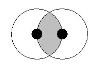
(b) $\beta=2$

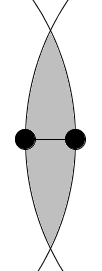
(c) $\beta=10$

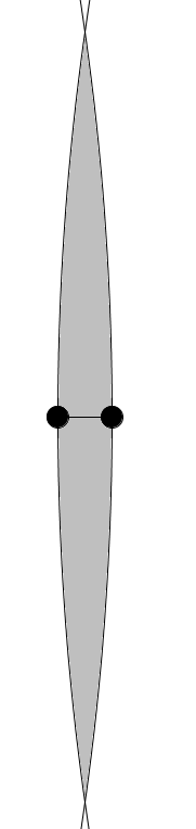
(d) $\beta=100$

Figure 1: Examples of lunes, $\beta$-neighbourhoods, of two planar points, black disks, for various values of $\beta$. The $\beta$-neighbourhoods are shaded in grey.

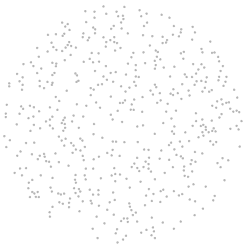
(a) $\mathbf{V}$

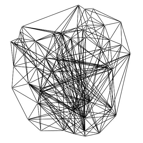
(b) $\beta=0.7$

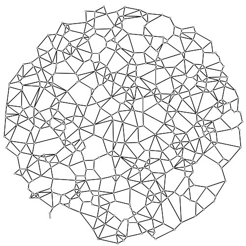
(c) $\beta=1$

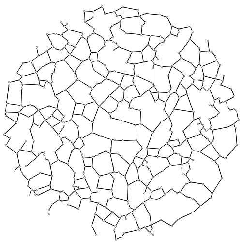
(d) $\beta=2$

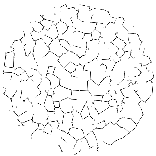
(e) $\beta=3$

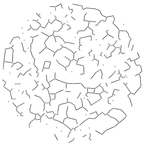
(f) $\beta=4$

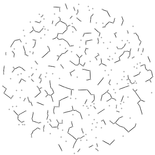
(g) $\beta=7$

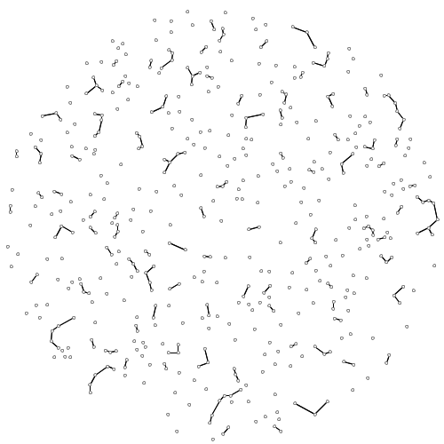
(h) $\beta=20$

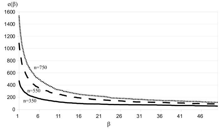
(i) $e(n,\beta)$

Figure 2: Example of $\beta$-skeletons of a random planar set. (a) A random planar set $\mathbf{V}$ of 500 discs, radius 2.5 each, randomly distributed in a disc radius 250. (b–h) Examples of $\beta$-skeletons on planar set $\mathbf{V}$. (i) Example power curves of edge loss, $e(n,\beta)$ is a number of edges in $\beta$-skeleton constructed on a random set with $n$ nodes, $1\leq\beta\leq 100$, $n=350$ (solid line), $n=550$ (dashed line) and $n=750$ (fine dashed line), values of $\beta$ are incremented by 0.1.

Given a set $\mathbf{V}$ of planar points, for any two points $p$ and $q$ we define a $\beta$-neighbourhood $U_{\beta}(p,q)$ as the intersection of two discs with radius $\beta|p-q|/2$ centered at points $((1-\frac{\beta}{2})p,\frac{\beta}{2}q)$ and $(\frac{\beta}{2}p,(1-\frac{\beta}{2})q)$, $\beta\geq 1$ [20, 16], see examples of the lunes in Fig. 1. Points $p$ and $q$ are connected by an edge in $\beta$-skeleton if the pair’s $\beta$-neighbourhood contains no other points from $\mathbf{V}$.

A $\beta$-skeleton is a graph $\mathbf{B}_{\beta}({\mathbf{V}})=\langle{\mathbf{V}},{\mathbf{E}},\beta\rangle$, where nodes ${\mathbf{V}}\subset{\mathbf{R}}^{2}$, edges $\mathbf{E}$, and for $p,q\in{\mathbf{V}}$ edge $(pq)\in\mathbf{E}$ if $U_{\beta}(p,q)\cap{\mathbf{V}}/\{p,q\}=\emptyset$. Parameterisation $\beta$ is monotonous: if $\beta_{1}>\beta_{2}$ then $\mathbf{B}_{\beta_{1}}({\mathbf{V}})\subset\mathbf{B}_{\beta_{2}}({\mathbf{V}})$ [16, 20].

A $\beta$-skeleton is a non-planar graph for $\beta<1$, see example in Fig. 2b. Therefore we consider only skeletons with $\beta>1$.

3 On stability of $\beta$-skeletons

$\beta$-skeletons of random planar sets lose their edges by a power law when $\beta$ increases linearly, see details in [4]. See examples of $\beta$-skeletons, $\beta=$1, 2, 3, 4, 7, 20, 100 and edge loss curve in Fig. 2. Most $\beta$-skeleton lose their edges with increase of $\beta$ however some $\beta$-skeleton do not. A stable $\beta$-skeleton retains its edges for any value of $\beta>1$. A most obvious example of a stable $\beta$-skeleton is a skeleton built on a set of planar points arranged in a rectangular array.

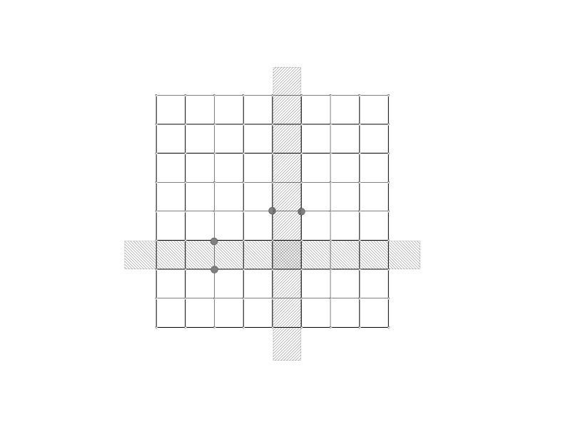
Figure 3: Rectangular lattice is a stable $\beta$-skeleton. $\beta$-neighbourhoods, $\beta\rightarrow\infty$, of two pairs of nodes (marked by grey discs) are shown by hatched areas.

Proposition 1

Rectangular lattice is a stable $\beta$-skeleton.

This is because when $\beta$ tends to infinity the $\beta$-neighbourhood tends to a rectangular shape and becomes an intersection of two half-planes. In details, let $\mathbf{H}_{ab}$ be an open half-plane bounded by an infinite straight line $l_{a}$ passing through $a$, perpendicular to segment $(a,b)$ and containing $b$; and $\mathbf{H}_{ba}$ be an open half-plane bounded by an infinite straight line $l_{b}$ perpendicular to segment $(a,b)$, passing through $b$ and containing $a$. Let $\mathbf{M}_{ab}=\mathbf{H}_{ab}\cap\mathbf{H}_{ba}$. When $\beta$ becomes extremely large, tends to infinity, a $\beta$-neighbourhood of any two neighbouring points $a$ and $b$ tends to $\mathbf{M}_{ab}$. A $\beta$-skeleton of planar set $\mathbf{V}$ is stable if for any $a,b\in\mathbf{V}$ $\mathbf{M}_{ab}$ does not contain any points from $\mathbf{V}$ apart of $a$ and $b$. The rectangular $\beta$-skeleton conserves its edges for any value of $\beta$ (Fig. 3). The rectangular lattice is stable because for any two neighbouring nodes $a$ and $b$ intersection $\mathbf{M}_{ab}$ of their half-planes fits between rows or columns of nodes without covering any other nodes.

Given $\beta$, is it possible to generate a planar set which $\beta$-skeleton is a connected graph? A method of growing such sets, and their $\beta$-skeletons, is presented further.

4 Growing $\beta$-skeletons

A graph is connected if there is a path along edges of the graph between any two nodes of the graph. An indirected graph is connected if there are no isolated nodes. To grow a connected $\beta$-skeleton for a given value of $\beta$ we start with a single planar point $p_{0}=(x_{0},y_{0})$ and then introduce additional points one by one. When a new candidate point is introduced to a planar set we check if

• the candidate point does not fell into $\beta$-neighbourhoods of existing nodes, and

• the skeleton of the planar set with the candidate point retains its connectivity, i.e. there are no isolated nodes.

Points can be added to the planar set either in a random fashion or in a regular manner. We adopt a regular addition of nodes by the following procedure.

Node Addition Procedure

1. $r=5,\theta=0,\delta=10$

2. $p=(x_{0}+r\cos\theta,y_{0}+r\sin\theta)$

3. if $\mathbf{B}_{\beta}(\mathbf{V}\cup\{p\})$ is connected graph and $(\forall q\in\mathbf{V}:|p-q|>\delta)$
   then $\mathbf{V}\leftarrow\mathbf{V}\cup\{p\}$

4. $\theta\leftarrow\theta+\Delta\theta$

5. if $\theta>360$ then $\theta\leftarrow 0$ and $r\leftarrow r+\Delta r$

6. go to step 2

We use polar coordinates $p=(x_{0}+r\cos\theta,y_{0}+r\sin\theta)$ and assume that no two points can lie closer than $\delta$ to each other, in all experiments $\delta=2.5$. Position of initial point is fixed, $p_{0}=(x_{0},y_{0})$. First candidate point is placed at distance $r$ from $p_{0}$ with angle $\theta=0$. The angle $\theta$ is incremented by $\Delta\theta$. When angle $\theta$ reaches 360 degrees radius $r$ is incremented by $\Delta r$ and $\theta$ is assigned value 0. The iterations may continue indefinitely but in experiments illustrated here we stop growing skeletons when $r$ reached 90. Further in the paper we sometimes address $\beta$-skeletons grown by above procedure as simply $\beta$-skeleton.

Proposition 2

Let $\Delta\theta\rightarrow 0$ then grown $\beta$-skeleton is transformed from a hexagonal lattice, for $\beta=1$, to an orthogonal lattice, for $\beta\rightarrow\infty$.

For $\beta=1$ lune $U_{\beta}(p,q)$ is disc with diameter $pq$ (Fig. 1a). Thus, in principle, we can arrange any number of points around an initial point $p_{0}$. However, due to imposed minimal distance $\delta=2.5$ between any two points, the points can be considered as discs. A hexagonal packing is a densest arrangement of identical discs. Rectangular lattice is a stable $\beta$-skeleton, it remains connected for arbitrarily large $\beta$.

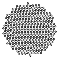
(a) $\beta=1$

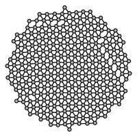
(b) $\beta=1.5$

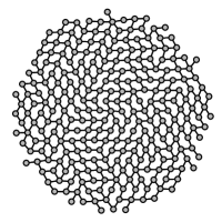
(c) $\beta=2$

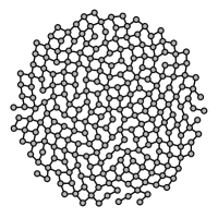
(d) $\beta=2.5$

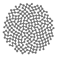
(e) $\beta=3$

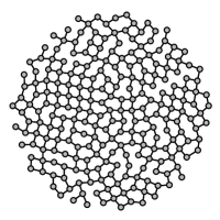
(f) $\beta=3.5$

(g) $\beta=4$

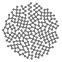
(h) $\beta=4.5$

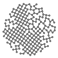
(i) $\beta=10$

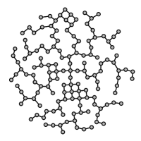
(j) $\beta=30$

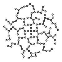
(k) $\beta=40$

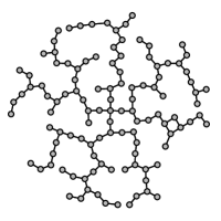
(l) $\beta=50$

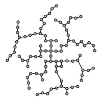
(m) $\beta=100$

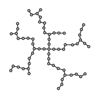
(n) $\beta=200$

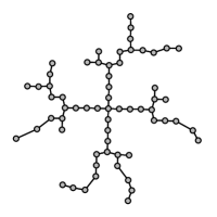
(o) $\beta=300$

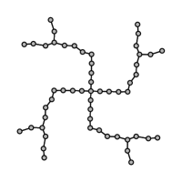
(p) $\beta=400$

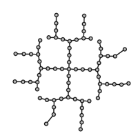
(q) $\beta=500$

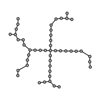
(r) $\beta=600$

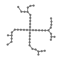
(s) $\beta=700$

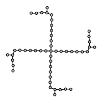
(t) $\beta=800$

Figure 4: Examples of $\beta$-skeletons grown from a single point, $r=5,\Delta r=0.5,\Delta\theta=0.5,\delta=2.5$

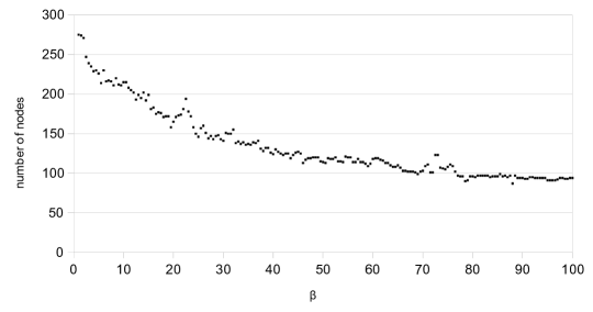
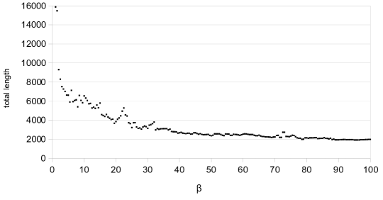
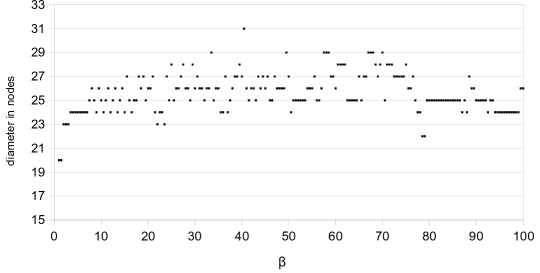
Figure 5: Average degree (a), number of nodes (b), total lengths of edges (c), and diameter in nodes (d) of $\beta$-skeletons grown with parameters $r=5,\Delta r=0.5,\Delta\theta=0.5,\delta=2.5$.

5 Dynamics of skeletons controlled by $\beta$

Skeletons grown on computers are never ideal, and never become rectangular lattices, due to impurities in their topologies introduced by increments of $\theta$. Examples of $\beta$-skeletons grown from a single point with angular increment $\Delta\theta=0.5$ are shown in Fig. 4. A hexagonal arrangement of nodes in $\beta$-skeleton for $\beta=1$ is well seen (Fig. 4a). The hexagonal arrangement is gradually destroyed when $\beta$ increases from 1 to 2 (Fig. 4abc) with majority of nodes having three or four neighbours (Fig. 5a).

Further increase of $\beta$ leads to dissociation of cycles and formation of tree-like skeletons with domains of lattice-like arrangements (Fig. 4i–t). Sizeable domains of rectangular lattices are still observed at $\beta=10$, e.g. domains located in southern, western and north-westerns parts of the graph in Fig. 4i. Branching of the tree is reduced with increase of $\beta$ till skeleton is transformed to a cross-like structures with a single binary branching at each of four main branches (Fig. 4t). This $\beta$-induced transformation is reflected in decrease in average degree of the graphs’ nodes, which almost stabilises around value 2 when $\beta$ exceeds 50 (Fig. 5a).

These structural transformations are reflected in decrease of a total number of nodes (Fig. 5b) and total length of edges (Fig. 5c). Increase of $\beta$ does not affect diameters of the $\beta$-skeletons, which vary between 23 and 29 nodes for $1\leq\beta\leq 100$ (Fig. 5d).

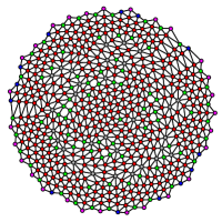
(a) $\Delta\theta=5$, $\beta=1$

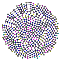
(b) $\Delta\theta=5$, $\beta=2$

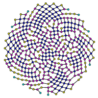
(c) $\Delta\theta=5$, $\beta=3$

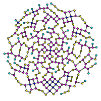
(d) $\Delta\theta=5$, $\beta=10$

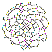
(e) $\Delta\theta=5$, $\beta=15$

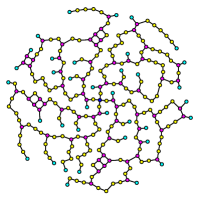
(f) $\Delta\theta=5$, $\beta=20$

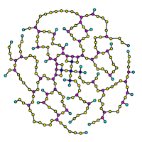
(g) $\Delta\theta=5$, $\beta=25$

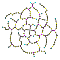
(h) $\Delta\theta=5$, $\beta=30$

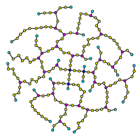
(i) $\Delta\theta=5$, $\beta=35$

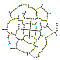
(j) $\Delta\theta=5$, $\beta=40$

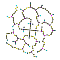
(k) $\Delta\theta=5$, $\beta=45$

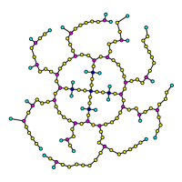
(l) $\Delta\theta=5$, $\beta=50$

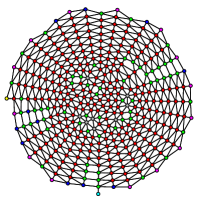
(m) $\Delta\theta=10$, $\beta=1$

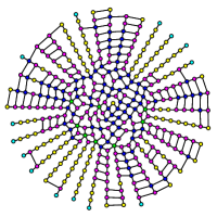
(n) $\Delta\theta=10$, $\beta=2$

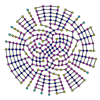
(o) $\Delta\theta=10$, $\beta=3$

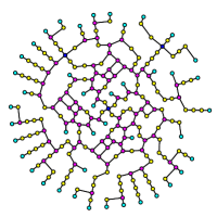
(p) $\Delta\theta=10$,$\beta=10$

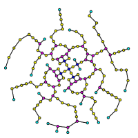
(q) $\Delta\theta=10$,$\beta=20$

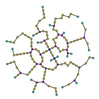
(r) $\Delta\theta=10$, $\beta=30$

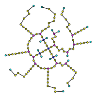
(s) $\Delta\theta=10$, $\beta=40$

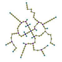
(t) $\Delta\theta=10$, $\beta=50$

Figure 6: $\beta$-skeletons grown with $\Delta\theta=5$ (a–l) and $\Delta\theta=10$ (m–t).

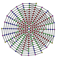
(a) $\Delta\theta=15$, $\beta=1$

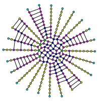
(b) $\Delta\theta=15$, $\beta=2$

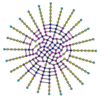
(c) $\Delta\theta=15$, $\beta=3$

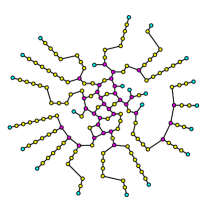
(d) $\Delta\theta=15$, $\beta=10$

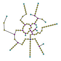
(e) $\Delta\theta=15$, $\beta=20$

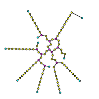
(f) $\Delta\theta=15$, $\beta=30$

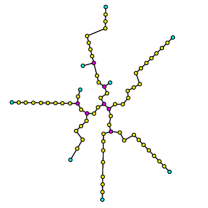
(g) $\Delta\theta=15$, $\beta=40$

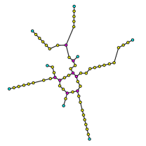
(h) $\Delta\theta=15$, $\beta=50$

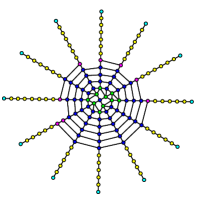
(i) $\Delta\theta=30$, $\beta=1$

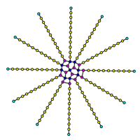
(j) $\Delta\theta=30$, $\beta=2$

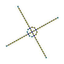
(k) $\Delta\theta=30$, $\beta=10$

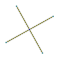
(l) $\Delta\theta=30$, $\beta\geq 26$

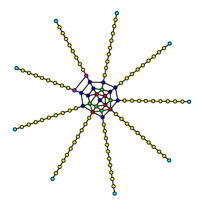
(m) $\Delta\theta=40$, $\beta=1$

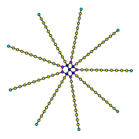
(n) $\Delta\theta=40$, $\beta=2$

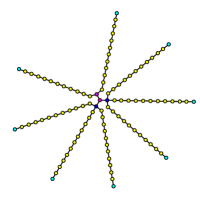
(o) $\Delta\theta=40$, $\beta=6$

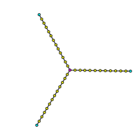
(p) $\Delta\theta=40$, $\beta=9$

Figure 7: $\beta$-skeletons grown with $\Delta\theta=15$ (a–h), $\Delta\theta=30$ (i–l) and $\Delta\theta=40$ (m–p).

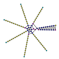
(a) $\Delta\theta=50$, $\beta=1$

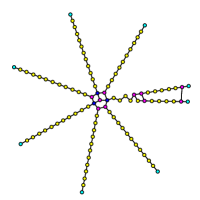
(b) $\Delta\theta=50$, $\beta=2$

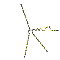
(c) $\Delta\theta=50$, $\beta=10$

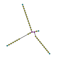
(d) $\Delta\theta=50$, $\beta\geq 30$

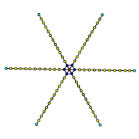
(e) $\Delta\theta=60$, $\beta=1$

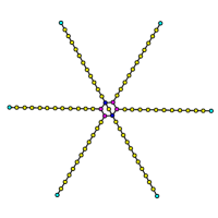
(f) $\Delta\theta=60$, $\beta=2$

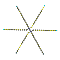
(g) $\Delta\theta=60$, $\beta\geq 3$

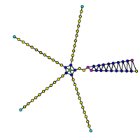
(h) $\Delta\theta=70$, $\beta=1$

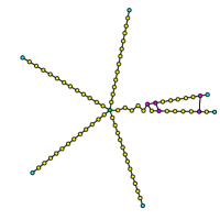
(i) $\Delta\theta=70$, $\beta=2$

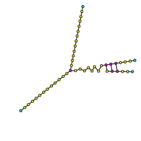
(j) $\Delta\theta=70$, $\beta=3$

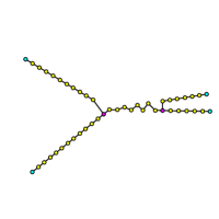
(k) $\Delta\theta=70$, $\beta\geq 8$

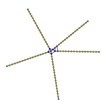
(l) $\Delta\theta=80$, $\beta=1$

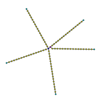
(m) $\Delta\theta=80$, $\beta=2$

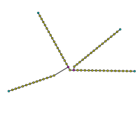
(n) $\Delta\theta=80$, $\beta=6$

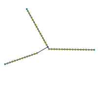
(o) $\Delta\theta=80$, $\beta\geq 9$

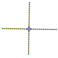
(p) $\Delta\theta=90$, $\beta=1$

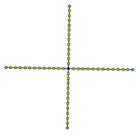
(q) $\Delta\theta=90$, $\beta>1$

Figure 8: $\beta$-skeletons grown with $\Delta\theta=50$ (a–d), $\Delta\theta=60$ (e–g), $\Delta\theta=70$ (h–k), $\Delta\theta=80$ (l–o) and $\Delta\theta=90$ (pq).

6 $\Delta\theta$ influences morphologies

Morphologies of $\beta$-skeletons are affected not only by values of $\beta$ but also $\Delta\theta$. We can expect that with increase of $\Delta\theta$ the skeletons converge from almost regular lattices to trees for $\beta<4$. For example, compare skeletons grown for $\Delta\theta=5$ (Fig. 6a–l) and $\Delta\theta=10$ (Fig. 6m–t). Increase of $\Delta\theta$ causes predominant decrease of lateral (aligned along concentric cycles centred in $p_{0}$) edges, see e.g. Fig. 6abc and Fig. 6mno, and decrease in branching of trees, see e.g. Fig. 6jkl and Fig. 6rst. New nodes are added to $\beta$-skeletons in a cycle of iterations, change of $\theta$ from 0 to 360, thus branches of the graphs are leaned towards circular arrangements (Fig. 6klrs).

For $\beta$ up to 3, $\beta$-skeletons consist of two morphologically distinctive components: internal core of a quasi-regular network and spider-web like halo of radial rays connected by lateral links. The pronounced examples of this morphological division are shown in Fig. 6mno and Fig. 7ab.

Increase of $\Delta\theta$ leads to a disappearance of lateral links and shrinking of the quasi-regular network core, see transition from Fig. 6m to Fig. 7a to Fig. 7i. Skeletons grown with large angle increments $\Delta\theta$ are characterised by a prevalence of radial edges, or rays. Thus, for $\Delta\theta=30$ we observe transition from a small spider web when $\beta=1$ (Fig. 7i) to twelve rays, $\beta=2$ (Fig. 7j), and four rays, $\beta\geq 26$ (Fig. 7j), structures. Number of rays is changed from nine, $\beta=2$, to seven, $\beta=6$, to three, $\beta=9$ (Fig. 7nop). Skeletons grown with large angular increments, $\Delta\theta=80$ and $90$, Fig. 8l–q consist of three, four or five rays, for any value of $\beta$.

In situations when $360\mod\Delta\theta>0$ lateral edges are formed between rays. Examples are $\beta$-skeletons grown with $\Delta\theta=50$ (Fig. 8ab) and $\Delta\theta=50$ (Fig. 8hij.)

7 Possible applications in sciences

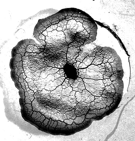
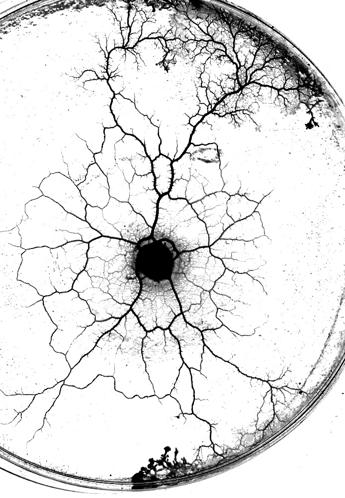
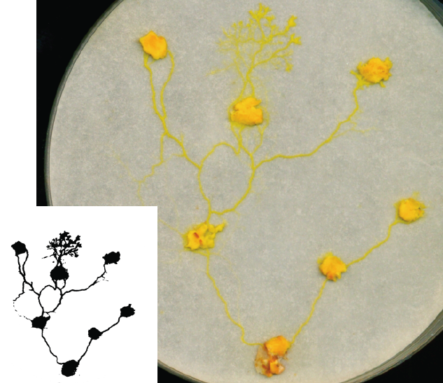
Figure 9: Slime mould P. polycephalum growing on a corn meal 2% agar gel (a), non-nutrient 2% agar gel (b), and a slightly wet filter paper (c). See details in [2].

Some aspects of a morphological dynamic of $\beta$-skeletons, controlled by $\beta$ and $\Delta\theta$, resemble substrate-induced morphological transformations in bacterial [14] and myxomycetes [2] colonies. Typically, a high concentration of nutrients in a growth substrate leads to formation of dense quasi-uniform omni-directionally propagating patterns. A low concentration of nutrients in a substrate leads to formation of branching tree-like structures. Two examples are shown in Fig. 9.

When plasmodium of P. polycephalum is inoculated on an agar plate with high concentration of nutrients (2% corn meal agar) the plasmodium’s growth-front propagates similarly to a circular wave. A dense network of protoplasmic tubes is formed inside the plasmodium’s body (Fig. 9a). Such growing pattern might be matched well by $\beta$-skeletons grown by the Node Addition Procedure, given in Sect. 4, with $\Delta\theta=0.5$, $1\leq\beta\leq 3.5$ (Fig. 4a–f), and $\Delta\theta=5$, $1\leq\beta\leq 3$ (Fig. 6abc) and $\Delta\theta=10$, $1\leq\beta\leq 3$ (Fig. 6mno).

On a non-nutrient 2% agar plasmodium forms a tree like structure (Fig. 9b). The plasmodium trees are alike $\beta$-skeletons generated with $\Delta\theta=0.5$, $30\leq\beta\leq 50$ (Fig. 4jkl), $\Delta\theta=5$, $30\leq\beta\leq 50$ (Fig. 6h–l), $\Delta\theta=10$, $20\leq\beta\leq 40$ (Fig. 6qrs). A degree of branching, or ’bushiness’, of protoplasmic trees decreases with increase of harshness of a growth substrate. For example, plasmodium cultivated on a filter paper, instead of agar gel, produces protoplasmic trees with very low degree of branching (Fig. 9c). Protoplasmic trees grown in a harsh conditions resemble $\beta$-skeletons grown with $\Delta\theta=0.5$, $600\leq\beta\leq 800$ (Fig. 4rst), $\Delta\theta=15$, $10\leq\beta\leq 50$ (Fig. 6d-h).

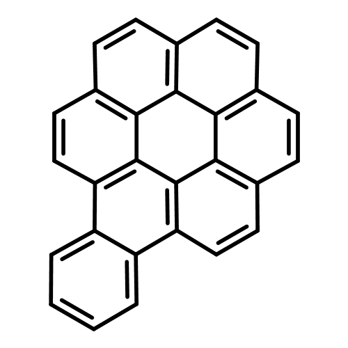
Figure 10: (a) Benzocoronene, (b) PAMAM-OS-trimethoxysilyl dendrimer. (c) Tetrakis(4-poly(nitriromethylene-bis(p-phenylene))phenyl)methane dendrimer generation 4. Chemical structures are drawn with www.chemspider.com.

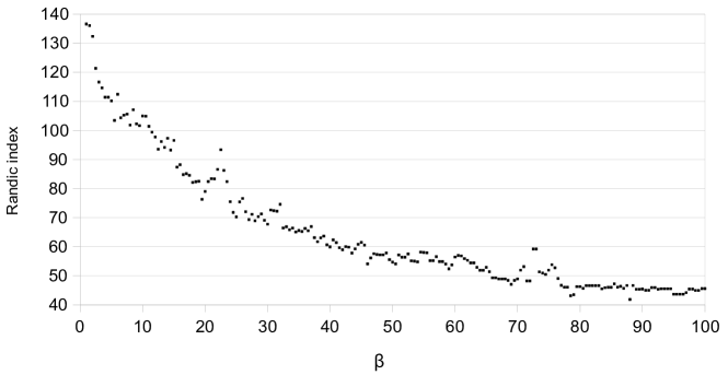
Figure 11: Randić index of $\beta$-skeletons grown with $r=5$, $\Delta r=0.5$, $\Delta\theta=0.5$, $\delta=2.5$

The procedure of growing $\beta$-skeletons may distantly pass for, at least at a very abstract level, a synthesis of cyclic (Fig. 10a) and dendrimer molecules (Fig. 10bc). Skeletons grown with low values of $\Delta\theta$ and $\beta$ may be considered analogous to cyclic molecules and skeletons produced with high values of $\Delta\theta$ and $\beta$ are alike dendrimer molecules.

Whilst no direct matching between $\beta$-skeletons and cyclic or dendrimer molecules can be demonstrated we calculated Randić index [28] of the $\beta$-skeletons grown for $\beta$ up to 100 (Fig. 11). The Randić index [28] is calculated as $R=\sum_{ij}C_{ij}*(\frac{1}{\sqrt{(d_{i}*d_{j})}})$, where $C_{ij}$ is an adjacency matrix of a graph.

The Randić index $R$ (originally called by Milan Randić as molecular branching index) [28] characterises relationships between structure, property and activity of molecular components [11]. There are proven linear relations between the Randić index and molecular polarisability, enthalpy of formation, molar refraction, van der Waals areas and volumes, chromatographic retention index [19], cavity surface areas calculated for water solubility of alcohols and hydrocarbons, biological potencies of anaesthetics [18], water solubility and boiling point [15] and even bio-concentration factor of hazardous chemicals [30]. Estrada [12] suggested the following structural interpretation: the Randić index is proportional to an area of molecular accessibility, i.e. area ’exposed’ to outside environment. The Randić index decreases with increase of $\beta$. Exposure of $\beta$-skeletons is proportional to $\beta$. This is how properties of the molecules imitated by $\beta$-skeletons will change when a molecule is transformed from, e.g. aromatic to dendritic.

8 Summary

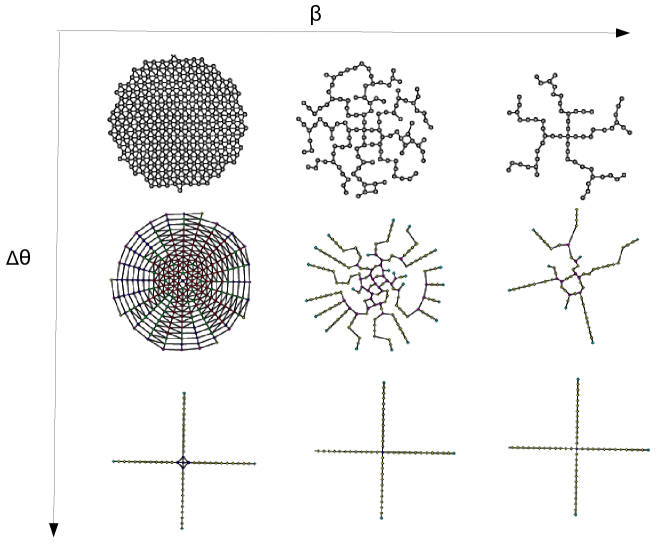
Figure 12: Evolution of grown $\beta$-skeletons.

Given a random planar set, a $\beta$-skeleton of the set is, in general, a disconnected graph for $\beta>2$. We presented a procedure for growing the $\beta$-skeletons which remain connected for any, yet specified during the growth, value of $\beta$ however large it is. In computational experiments we demonstrated that with increase of $\beta$ and/or decrease of approximation accuracy, $\Delta\theta$, the skeletons undergo a transformation from almost regular lattices or networks to branching trees to cross-like graphs (Fig. 12). We speculate that such evolution of the $\beta$-skeletons somewhat imitates morphological transformations of myxomycetes and bacterial colonies governed by concentration of nutrients in their growth substrates and transformation of molecules from aromatic to dendritic forms.

References

- [1] Adamatzky A. Developing proximity graphs by Physarum Polycephalum: Does the plasmodium follow Toussaint hierarchy? Parallel Processing Letters 19 (2008) 105–127.
- [2] Adamatzky A. Physarum Machines (World Scientific, 2010).
- [3] Adamatzky A. (Ed.) Bioevaluation of World Transport Networks (World Scientific, 2012).
- [4] Adamatzky A. How -skeletons lose their edges. Submitted (2012).
- [5] Amenta N., Bern M., Eppstein D. The Crust and the -Skeleton: Combinatorial Curve Reconstruction. Graphical Models and Image Processing. 60 (1998) 125–135.
- [6] Beavon D. J. K., Brantingham P. L. and Brantingham P. J. The influence of street networks on the patterning of property offenses. www.popcenter.org/library/CrimePrevention/Volume_02/06beavon.pdf
- [7] Billiot J. M., Corset F., Fontenas E. Continuum percolation in the relative neighbourhood graph. arXiv:1004.5292
- [8] Dale M. R. T. Spatial Analysis in Plant Ecology (Cambridge University Press, 2000).
- [9] Dale M. R. T., Dixon P., Fortin M.-J., Legendre P., Myers D. E. and Rosenberg M. S. Conceptual and mathematical relationships among methods for spatial analysis. Ecography 25 (2002) 558- 577.
- [10] Delaunay B. Sur la sphère vide, Izvestia Akademii Nauk SSSR, Otdelenie Matematicheskikh i Estestvennykh Nauk, 7 (1934) 793–800.
- [11] Estrada E. Generalization of topological indices. Chem. Phys. Lett. 336 (2001) 248–252.
- [12] Estrada E. The structural interpretation of the Randić index. Internet Electronic Journal of Molecular Design 1 (2002) 360–366.
- [13] Gabriel K. R. and Sokal R. R. A new statistical approach to geographic variation analysis. Systematic Zoology 18 (1969) 259 -270.
- [14] Golding I., Kozlovsky Y., Cohen I., Ben-Jacob E. Studies of bacterial branching growth using reaction diffusion models for colonial development Physica A 260 (1998) 510–554.
- [15] Hall L.H., Kier L.B. , Murray W.J. Molecular connectivity. II. Relationship to water solubility and boiling point. J. Pharm. Sci. 64 (1975) 1974–1977.
- [16] Jaromczyk J. W. and G. T. Toussaint, Relative neighborhood graphs and their relatives. Proc. IEEE 80 (1992) 1502–1517.
- [17] Jombart T., Devillard S., Dufour A.-B., Pontier D. Revelaing cryptic spatial patterns in genetic variability by a new multivariate method. Heredity 101 (2008) 92–103.
- [18] Kier L.B., Hall L.H., Murray W.J., Randić M., Molecular connectivity. I. Relationship to nonspecific local anesthesia, J. Pharm. Sci. 64 (1975) 1971–1974.
- [19] Kier, L. B.; Hall, L. H. Molecular Connectivity in Chemistry and Drug Research. Academic Press, 1976.
- [20] Kirkpatrick D.G. and Radke J.D. A framework for computational morphology. In: Toussaint G. T., Ed., Computational Geometry (North-Holland, 1985) 217- 248.
- [21] Legendre P. and Fortin M.-J. Spatial pattern and ecological analysis. Vegetatio 80 (1989) 107–138.
- [22] Li X.-Y. Application of computation geometry in wireless networks. In: Cheng X., Huang X., Du D.-Z. (Eds.) Ad Hoc Wireless Networking (Kluwer Academic Publishers, 2004) 197–264.
- [23] Li X., Shi Y., Wang L., An updated survey on the Randić index. Math. Chem. Monogr. (6) (2008) 9–4
- [24] Magwene P. W. Using correlation proximity graphs to study phenotypic integration. Evolutionary Biology. 35 (2008) 191–198.
- [25] Matula D. W. and Sokal R. R. Properties of Gabriel graphs relevant to geographic variation research and clustering of points in the plane. Geogr. Anal. 12 (1980) 205–222.
- [26] Muhammad R. B. A distributed graph algorithm for geometric routing in ad hoc wireless networks. J Networks 2 (2007) 49–57.
- [27] Plavsić D., Nikolić S., Trinajstić N. and Mihalić Z. On the Harary index for the characterization of chemical graphs. J. Math. Chem. 12 (1993) 235–250.
- [28] Randić, M. Characterization of molecular branching, Journal of the American Chemical Society 97 (1975) 6609–6615.
- [29] Runions A., Fuhrer M., Lane B., Federl P., Rolland-Lagan A.-G., and Prusinkiewicz P. Modeling and visualization of leaf venation patterns. ACM Transactions on Graphics 24 (2005) 702–711.
- [30] Sabljić A. and Protić M. Molecular connectivity: A novel method for prediction of bioconcentration factor of hazardous chemicals. Chemico-Biological Interactions 42 (1982) 301–310.
- [31] Santi P. Topology Control in Wireless Ad Hoc and Sensor Networks (Wiley, 2005).
- [32] Sokal R. R. and Oden N. L. Spatial autocorrelation in biology 1. Methodology. Biological Journal of the Linnean Society 10 (2008) 199–228.
- [33] Song W.-Z., Wang Y., Li X.-Y. Localized algorithms for energy efficient topology in wireless ad hoc networks. In: Proc. MobiHoc 2004 (May 24 -26, 2004, Roppongi, Japan).
- [34] Sridharan M. and Ramasamy A. M. S. Gabriel graph of geomagnetic Sq variations. Acta Geophysica (2010) 10.2478/s11600-010-0004-y
- [35] Toroczkai Z. and Guclu H. Proximity networks and epidemics. Physica A 378 (2007) 68. arXiv:physics/0701255v1
- [36] Wan P.-J., Yi C.-W. On the longest edge of Gabriel Graphs in wireless ad hoc networks. IEEE Trans. on Parallel and Distributed Systems 18 (2007) 111–125.
- [37] Watanabe D. A study on analyzing the road network pattern using proximity graphs. J of the City Planning Institute of Japan 40 (2005) 133–138.
- [38] Watanabe D. Evaluating the configuration and the travel efficiency on proximity graphs as transportation networks. Forma 23 (2008) 81–87.
- [39] Yang Y., Lu L. The Randić index and the diameter of graphs Discrete Mathematics 311 (2011) 1333 1343.