Quintessence: A Review

Abstract

Quintessence is a canonical scalar field introduced to explain the late-time cosmic acceleration. The cosmological dynamics of quintessence is reviewed, paying particular attention to the evolution of the dark energy equation of state $w$. For the field potentials having tracking and thawing properties, the evolution of $w$ can be known analytically in terms of a few model parameters. Using the analytic expression of $w$, we constrain quintessence models from the observations of supernovae type Ia, cosmic microwave background, and baryon acoustic oscillations. The tracking freezing models are hardly distinguishable from the $\Lambda$-Cold-Dark-Matter ($\Lambda$CDM) model, whereas in thawing models the today’s field equation of state is constrained to be $w_{0}<-0.7$ (95 % CL). We also derive an analytic formula for the growth rate of matter density perturbations in dynamical dark energy models, which allows a possibility to put further bounds on $w$ from the measurement of redshift-space distortions in the galaxy power spectrum. Finally we review particle physics models of quintessence–such as those motivated by supersymmetric theories. The field potentials of thawing models based on a pseudo-Nambu-Goldstone boson or on extended supergravity theories have a nice property that a tiny mass of quintessence can be protected against radiative corrections.

1 Introduction

The observational discovery of the late-time cosmic acceleration from the Supernovae type Ia (SN Ia) opened up a new research area in modern cosmology [1, 2]. About 70 % of the energy density of the Universe today consists of an unknown component called dark energy. This has been also confirmed by other observations– such as Cosmic Microwave Background (CMB) [3, 4] and Baryon Acoustic Oscillations (BAO) [5]. The property of dark energy is characterized by the equation of state $w=P/\rho$, where $P$ is the pressure and $\rho$ is the energy density. Dark energy has a negative pressure with $w$ less than $-1/3$.

One of the simplest candidates of dark energy is the cosmological constant $\Lambda$ with $w=-1$. The cosmological constant can arise from a vacuum energy in particle physics, but its energy scale is enormously larger than the observed energy scale of dark energy [6]. There have been many attempts to construct de Sitter vacua in supersymmetric theories. In string theory, for example, huge numbers of de Sitter vacua ($\sim 10^{500}$) can be present after the so-called flux compactification of higher-dimensional manifolds [7]. We may live in a vacuum with a tiny vacuum energy, but it is generally difficult to justify the reason for living such a specific vacuum unless some anthropic principle is introduced. So far, it is fair to say that there is no satisfactory scenario where the small energy scale of dark energy can be naturally explained by the vacuum energy related to particle physics.

If the cosmological constant problem is solved in a way that it vanishes completely, we need to find out an alternative mechanism to explain the origin of dark energy [8, 9]. Broadly speaking, we can classify dark energy models into two classes. The first one is based on a specific form of matter– such as quintessence [10, 11, 12, 13, 14, 15, 16], k-essence [17, 18], and the Chaplygin gas [19]. The second one is based on the modification of gravity at large distances (see Refs. [20] for reviews). In both classes the dark energy equation of state dynamically changes in time, by which the models can be distinguished from the $\Lambda$CDM model.

Quintessence is described by a canonical scalar field $\phi$ minimally coupled to gravity. Compared to other scalar-field models such as phantoms and k-essence, quintessence is the simplest scalar-field scenario without having theoretical problems such as the appearance of ghosts and Laplacian instabilities. A slowly varying field along a potential $V(\phi)$ can lead to the acceleration of the Universe. This mechanism is similar to slow-roll inflation in the early Universe, but the difference is that non-relativistic matter (dark matter and baryons) cannot be ignored to discuss the dynamics of dark energy correctly. Moreover, the energy scale of the quintessence potential needs to be of the order of $\rho_{\rm DE}\approx 10^{-47}$ GeV⁴ today, which is much smaller than that of the inflaton potential.

The dynamics of quintessence in the presence of non-relativistic matter has been studied in detail for many different potentials [14, 15, 16, 21, 22, 23, 24, 25]. Depending on the evolution of $w$, we can broadly classify quintessence models into two classes [24]: (i) thawing models and (ii) freezing models. In the first class, the field is nearly frozen by a Hubble friction during the early cosmological epoch and it starts to evolve once the field mass drops below the Hubble expansion rate. In the second class, the evolution of the field gradually slows down because the potential tends to be shallow at late times. For the inverse power-law potential $V(\phi)=M^{4+p}\phi^{-p}$ ($p>0$), there is so-called a tracker solution [26] along which $w$ is nearly constant during the matter era and $w$ starts to decrease after that. This case belongs to a subclass of freezing models. For thawing and tracker models there exist convenient analytic formulas of $w$ [27, 28, 29, 30] employed to test the models with the data of distance measurements of SN Ia, CMB, and BAO.

The redshift-space distortions (RSD) appearing in clustering pattern of galaxies [31, 32] can provide additional constraints on the growth rate of matter perturbations $\delta_{m}$. Since the evolution of $\delta_{m}$ is different depending on the field equation of state [33, 34, 35], it is possible to place bounds on $w$ from the data of RSD. In fact there exist analytic formulas of $\delta_{m}$ and its growth rate [36], which can be used to constrain quintessence models.

In order to realize the cosmic acceleration today, the mass $m_{\phi}$ of quintessence (defined by $m_{\phi}^{2}=d^{2}V(\phi)/d\phi^{2}$) needs to be extremely small, i.e., $|m_{\phi}|\lesssim H_{0}\approx 10^{-33}$ eV, where $H_{0}$ is the today’s Hubble parameter. In general there is a difficulty to reconcile such a ultra light mass with the energy scales appearing in particle physics [37]. Moreover, in the absence of some symmetry, the radiative corrections may disrupt the flatness of the quintessence potentials required for the cosmic acceleration [38]. However, it is not entirely hopeless to construct viable quintessence models in the framework of particle physics [39, 40, 41, 42, 43, 44, 45, 46, 47].

In this article, we review several cosmological aspects of quintessence– including its cosmological dynamics, analytic solutions of $w$, observational constraints, and particle physics models. The review is organized as follows. In Sec. 2 we present the field equations of motion for general quintessence potentials and then proceed to the analysis of fixed points for exponential potentials. In Sec. 3 we classify quintessence potentials into two classes depending on the evolution of $w$ and then derive analytic solutions of $w$. These solutions are employed to put observational bounds on quintessence at the background level. In Sec. 4 we derive analytic formulas for the growth rate of matter density perturbations and discuss constraints on some of quintessence models from the recent data of RSD. In Sec. 5 we review theoretical models of quintessence based on supersymmetric theories. Sec. 6 is devoted to conclusions.

2 Dynamical equations of motion and exponential potentials

Let us consider quintessence in the presence of non-relativistic matter described by a barotropic perfect fluid. The total action is given by

$$S=\int d^{4}x\sqrt{-g}\left[\frac{1}{2}M_{\rm pl}^{2}R-\frac{1}{2}g^{\mu\nu}\partial_{\mu}\phi\partial_{\nu}\phi-V(\phi)\right]+S_{m}\,,$$ (1)

where $g$ is the determinant of the metric $g_{\mu\nu}$, $M_{\rm pl}$ is the reduced Planck mass, $R$ is the Ricci scalar, $S_{m}$ is the matter action. We assume that non-relativistic matter does not have a direct coupling to the quintessence field $\phi$.

We study the dynamics of quintessence on the flat Friedmann-Lemaître-Robertson-Walker (FLRW) background with the line element $ds^{2}=-dt^{2}+a^{2}(t)d{\bm{x}}^{2}$, where $a(t)$ is the scale factor with cosmic time $t$. The pressure and the energy density of quintessence are given, respectively, by $P_{\phi}=\dot{\phi}^{2}/2-V(\phi)$ and $\rho_{\phi}=\dot{\phi}^{2}/2+V(\phi)$, where a dot represents a derivative with respect to $t$. The dark energy equation of state is

$$w\equiv\frac{P_{\phi}}{\rho_{\phi}}=\frac{\dot{\phi}^{2}/2-V(\phi)}{\dot{\phi}^{2}/2+V(\phi)}\,.$$ (2)

The scalar field satisfies the continuity equation $\dot{\rho_{\phi}}+3H(\rho_{\phi}+P_{\phi})=0$, i.e.,

$$\ddot{\phi}+3H\dot{\phi}+V_{,\phi}=0\,,$$ (3)

where $H\equiv\dot{a}/a$ and $V_{,\phi}\equiv dV/d\phi$. For a matter fluid with the energy density $\rho_{m}$ and the equation of state $w_{m}$, the equations of motion following from the action (1) are

$$3M_{\rm pl}^{2}H^{2} = \dot{\phi}^{2}/2+V(\phi)+\rho_{m}\,,$$ (4)

$$2M_{\rm pl}^{2}\dot{H} = -\left[\dot{\phi}^{2}+(1+w_{m})\rho_{m}\right]\,.$$ (5)

In order to deal with the cosmological dynamics of this system, it is convenient to introduce the following dimensionless variables [14]

$$x\equiv\frac{\dot{\phi}}{\sqrt{6}M_{\rm pl}H}\,,\qquad y\equiv\frac{\sqrt{V(\phi)}}{\sqrt{3}M_{\rm pl}H}\,.$$ (6)

The field density parameter $\Omega_{\phi}\equiv\rho_{\phi}/(3M_{\rm pl}^{2}H^{2})$ can be expressed as $\Omega_{\phi}=x^{2}+y^{2}$. From Eq. (4) the matter density parameter $\Omega_{m}\equiv\rho_{m}/(3M_{\rm pl}^{2}H^{2})$ satisfies $\Omega_{m}=1-\Omega_{\phi}$. The field equation of state (2) reads $w=(x^{2}-y^{2})/(x^{2}+y^{2})$. We also define the effective equation of state $w_{\rm eff}\equiv-1-2\dot{H}/(3H^{2})$, where $\dot{H}/H^{2}$ can be evaluated from Eq. (5) as

$$\frac{\dot{H}}{H^{2}}=-3x^{2}-\frac{3}{2}(1+w_{m})(1-x^{2}-y^{2})\,.$$ (7)

Taking the derivatives of $x$ and $y$ with respect to $N\equiv\ln a$ and using Eqs. (3) and (7), it follows that

$$\frac{dx}{dN} = -3x+\frac{\sqrt{6}}{2}\lambda y^{2}+\frac{3}{2}x\left[(1-w_{m})x^{2}+(1+w_{m})(1-y^{2})\right],$$ (8)

$$\frac{dy}{dN} = -\frac{\sqrt{6}}{2}\lambda xy+\frac{3}{2}y\left[(1-w_{m})x^{2}+(1+w_{m})(1-y^{2})\right]\,,$$ (9)

where $\lambda$ is defined by $\lambda\equiv-M_{\rm pl}V_{,\phi}/V$.

The models with constant $\lambda$ corresponds to the exponential potential [13, 14, 48]

$$V(\phi)=V_{0}e^{-\lambda\phi/M_{\rm pl}}\,,$$ (10)

in which case Eqs. (8) and (9) are closed. The fixed points of this system can be derived by setting $dx/dN=0$ and $dy/dN=0$ [14]:

• (a) $(x,y)=(0,0)$, $\Omega_{\phi}=0$,  $w_{{\rm eff}}=w_{m}$,  $w$ is undetermined.

• (b) $(x,y)=(\pm 1,0)$,  $\Omega_{\phi}=1$, $w_{{\rm eff}}=w=1$.

• (c) $(x,y)=(\lambda/\sqrt{6},[1-\lambda^{2}/6]^{1/2})$,  $\Omega_{\phi}=1$, $w_{{\rm eff}}=w=-1+\lambda^{2}/3$.

• (d) $(x,y)=(\sqrt{3/2}(1+w_{m})/\lambda,[3(1-w_{m}^{2})/2\lambda^{2}]^{1/2})$,
  $\Omega_{\phi}=3(1+w_{m})/\lambda^{2}$,  $w_{{\rm eff}}=w=w_{m}$.

If we consider non-relativistic matter ($w_{m}=0$), the matter-dominated epoch ($w_{\rm eff}\simeq 0,\Omega_{\phi}\ll 1$) can be realized either by (a) or (d). The point (d) is the so-called scaling solution [13, 14], along which the ratio $\Omega_{m}/\Omega_{\phi}\,(\neq 0)$ remains constant. In order to realize the matter-dominated epoch by the scaling solution, we require the condition $\lambda^{2}\gg 1$. On the other hand, under the condition $\lambda^{2}<2$, the epoch of cosmic acceleration ($w_{\rm eff}<-1/3$) can be realized by the point (c). This shows that the transition from (d) to (c) is not possible, but for $\lambda^{2}<2$ the system can evolve from (a) to (c). The radiation-dominated epoch corresponds to the fixed point (a) with $w_{\rm eff}=w_{m}=1/3$.

In order to study the stabilities of the fixed points $(x,y)=(x_{c},y_{c})$, we consider linear perturbations $\delta x$ and $\delta y$ about them. Then the perturbations satisfy the following differential equations

$$\frac{d}{dN}\left(\begin{array}[]{c}\delta x\\ \delta y\end{array}\right)={\cal M}\left(\begin{array}[]{c}\delta x\\ \delta y\end{array}\right)\,,\qquad{\cal M}=\left(\begin{array}[]{cc}\partial f_{1}/\partial x&\partial f_{1}/\partial y\\ \partial f_{2}/\partial x&\partial f_{2}/\partial y\end{array}\right)_{x=x_{c},\,y=y_{c}}\,,$$ (11)

where $f_{1}(x,y)$ and $f_{2}(x,y)$ are the r.h.s. of Eqs. (8) and (9) respectively. If both the eigenvalues $\mu_{1}$ and $\mu_{2}$ of the matrix ${\cal M}$ are negative, the corresponding fixed point is stable. If either $\mu_{1}$ or $\mu_{2}$ is negative, the point corresponds to a saddle. If both $\mu_{1}$ and $\mu_{2}$ are positive, the fixed point is unstable. For complex values of $\mu_{1}$ and $\mu_{2}$ with negative real parts, the fixed point is called a stable spiral.

The eigenvalues of the point (c) are $\mu_{1}=(\lambda^{2}-6)/2$ and $\mu_{2}=\lambda^{2}-3(1+w_{m})$ [14], so that it is stable under the condition $\lambda^{2}<3(1+w_{m})$ for $0\leq w_{m}\leq 1$. The condition for cosmic acceleration corresponds to $\lambda^{2}<2$, in which case the point (c) is stable. The eigenvalues of the point (a) are $\mu_{1}=-(3/2)(1-w_{m})$, $\mu_{2}=(3/2)(1+w_{m})$, so that it is a saddle for $0\leq w_{m}\leq 1$. This means that, for $\lambda^{2}<2$, the solution eventually exits the point (a) to approach the attractor point (c).

The dark energy equation of state $w$ for the point (a) is undetermined, but in the realistic Universe, $x$ and $y$ are not exactly 0. The early evolution of $w$ depends on the initial conditions of $x$ and $y$. If $x^{2}\gg y^{2}$ and $x^{2}\ll y^{2}$, we have $w\simeq 1$ and $w\simeq-1$ respectively. Finally the solution approaches the constant value $w=-1+\lambda^{2}/3$. Since $w$ dynamically changes in this way, the quintessence model with the exponential potential is observationally distinguishable from the $\Lambda$CDM model.

For quintessence models in which $\lambda$ is not constant, Eqs. (8) and (9) are not closed. In such cases the situation is more involved, but it is possible to derive analytic solutions of $w$ by classifying quintessence potentials according to the evolution of $w$. In the next section we shall address this issue.

3 Classification of quintessence models and observational constraints

In order to study the evolution of $w$ for the models with varying $\lambda$, we derive the differential equations for $w$ and $\Omega_{\phi}$. Using Eqs. (7)-(9), we obtain

$$w^{\prime} = (w-1)[3(1+w)-\lambda\sqrt{3(1+w)\Omega_{\phi}}]\,,$$ (12)

$$\Omega_{\phi}^{\prime} = -3(w-w_{m})\Omega_{\phi}(1-\Omega_{\phi})\,,$$ (13)

where a prime represents a derivative with respect to $N=\ln a$. Introducing the quantity $\Gamma\equiv VV_{,\phi\phi}/V_{,\phi}^{2}$, the parameter $\lambda$ obeys

$$\lambda^{\prime}=-\sqrt{3(1+w)\Omega_{\phi}}\,(\Gamma-1)\lambda^{2}\,.$$ (14)

The evolution of $w$ is different depending on the quintessence potentials and the initial conditions. In what follows we discuss three qualitatively different cases: (i) tracking freezing models, (iii) scaling freezing models, and (iii) thawing models. In freezing models the potential tends to be shallow at late times, which results in the decrease of $w$. In thawing models the mass of the field becomes smaller than $H$ only recently, so that the deviation of $w$ from $-1$ occurs at late times.

3.1 Tracking freezing models

For the field density parameter satisfying the relation

$$\Omega_{\phi}=3(1+w)/\lambda^{2}\,,$$ (15)

$w$ is constant from Eq. (12). If $w=w_{m}$, then $\Omega_{\phi}$ is constant from Eq. (13) and hence $\lambda$ is constant. This corresponds to the scaling solution (d) discussed in Sec. 2. Since the scaling solution is stable for $\lambda^{2}>3(1+w_{m})$ [14], it does not exit to the fixed point (c). If $\lambda$ decreases in time, the system can enter the epoch of cosmic acceleration. From Eq. (14) this condition translates into

$$\Gamma>1\,.$$ (16)

The solution (15) satisfying the condition (16) is called a tracker [26], along which $\Omega_{\phi}$ increases and hence $w<w_{m}$. The tracker corresponds to a common evolutionary trajectory that attracts the solutions with different initial conditions. From Eq. (15) we have the relation $\Omega_{\phi}^{\prime}/\Omega_{\phi}=-2\lambda^{\prime}/\lambda$. Using Eqs. (13) and (14) under the condition $\Omega_{\phi}\ll 1$, the constant equation of state along the tracker is [26]

$$w=w_{(0)}\equiv\frac{w_{m}-2(\Gamma-1)}{2\Gamma-1}\,.$$ (17)

For example, let us consider the inverse power-law potential [13]

$$V(\phi)=M^{4+p}\phi^{-p}\,,$$ (18)

where $M$ and $p~{}(>0)$ are constants. Since in this case $\Gamma=1+1/p>1$, the tracking condition (16) is satisfied. The constant equation of state (17) is $w_{(0)}=(p\,w_{m}-2)/(p+2)$ and hence $w_{(0)}=-2/(p+2)$ during the matter era. With the growth of $\Omega_{\phi}$, $w$ starts to decrease from $w_{(0)}$. Hence the tracker belongs to the class of freezing models.

Figure 1: The field equation of state $w$ versus $a$ for the tracker solution. This case corresponds to the inverse power-law potential $V(\phi)=M^{5}\phi^{-1}$. The solid curve is derived by solving Eqs. (12)-(14) numerically, whereas other curves show the 1-st, 2-nd, 3-rd order analytic solutions (21).

The analytic solution (17) is valid in the regime $\Omega_{\phi}\ll 1$. We take into account the variation of $w$ by dealing with $\Omega_{\phi}$ as a perturbation to the 0-th order solution (17). From Eqs. (12) and (14), the perturbation $\delta w$ around $w_{(0)}$ obeys [30]

$$a^{2}\frac{d^{2}\delta w}{da^{2}}+\frac{5-6w_{(0)}}{2}a\frac{d\delta w}{da}+\frac{9}{2}(1-w_{(0)})\delta w-\frac{9}{2}w_{(0)}(1-w_{(0)}^{2})\Omega_{\phi}(a)=0\,,$$ (19)

where we assumed that $\Gamma$ is nearly constant. For $\Omega_{\phi}(a)$ we use the 0-th order solution

$$\Omega_{\phi}(a)=\frac{\Omega_{\phi 0}\,a^{-3w_{(0)}}}{\Omega_{\phi 0}\,a^{-3w_{(0)}}+1-\Omega_{\phi 0}}\,,$$ (20)

where $\Omega_{\phi 0}$ is the today’s value of $\Omega_{\phi}$. Substituting Eq. (20) into Eq. (19), we obtain the following integrated solution [30]

$$w(a)=w_{(0)}+\sum_{n=1}^{\infty}\frac{(-1)^{n-1}w_{(0)}(1-w_{(0)}^{2})}{1-(n+1)w_{(0)}+2n(n+1)w_{(0)}^{2}}\left(\frac{\Omega_{\phi}(a)}{1-\Omega_{\phi}(a)}\right)^{n}\,.$$ (21)

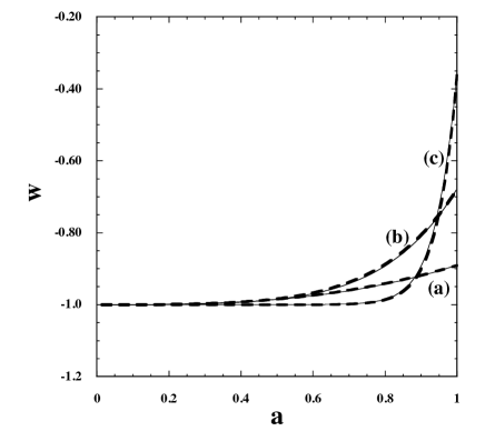
In Fig. 1 we plot the evolution of $w$ derived by the analytic solution (21) for the inverse power-law potential $V(\phi)=M^{5}\phi^{-1}$. Each curve corresponds to the 1-st, 2-nd, 3-rd order solution, whereas the solid curve is derived by solving Eqs. (12)-(14) numerically. We find that the analytic solution up to 3-rd order shows good agreement with the full numerical result. The analytic expression of $w$ is parametrized by two parameters $w_{(0)}$ and $\Omega_{\phi 0}$ alone.

The observational constraints on the tracker model have been carried out in Refs. [30, 49, 50]. In addition to the SN Ia data, the distance measurements of the CMB and BAO peaks provide the information of the background expansion history from the recombination epoch to today. From the joint data analysis of Union 2.1 [51], WMAP7 [52], and BAO (SDSS7 [53] and BOSS [54]), the tracker equation of state during the matter era is constrained to be $w_{(0)}<-0.964$ (95% CL) under the prior $w_{(0)}>-1$ [50]. For the potential (18) this bound translates into $p<0.075$. In Ref. [50] it was found that the best-fit corresponds to $w_{(0)}=-1$, i.e., the $\Lambda$CDM. If we do not put the prior $w_{(0)}>-1$, the best-fit model parameters are found to be $w_{(0)}=-1.097$ and $\Omega_{\phi 0}=0.717$. With the BOSS BAO data [54] the phantom equation of state ($w_{(0)}<-1$) is particularly favored, but this is not the regime of quintessence.

3.2 Scaling freezing models

The scaling solution [13, 14] can be regarded as a special case of a tracker along which $\Omega_{\phi}=3(1+w)/\lambda^{2}$ is constant. During the matter era, $w=w_{m}=0$ and hence $\Omega_{\phi}=3/\lambda^{2}$. Since $\lambda$ is constant, $\Gamma=1$ from Eq. (14). This case corresponds to the exponential potential (10), but the system does not enter the phase of cosmic acceleration because the field equation of state is the same as that of the background fluid.

This problem can be alleviated by considering the double exponential potential [55]

$$V(\phi)=V_{1}e^{-\lambda_{1}\phi/M_{\rm pl}}+V_{2}e^{-\lambda_{2}\phi/M_{\rm pl}}\,,$$ (22)

where $\lambda_{i}$ and $V_{i}$ ($i=1,2$) are constants (see Refs. [56, 57, 58] for related potentials). For the parameters satisfying the conditions $\lambda_{1}\gg 1$ and $\lambda_{2}\lesssim 1$, the solution first enters the scaling regime characterized by $\Omega_{\phi}=3(1+w_{m})/\lambda_{1}^{2}$. During the radiation era ($w_{m}=1/3$) the constraint coming from the big bang nucleosynthesis gives the bound $\Omega_{\phi}<0.045$ (95 % CL) [59], which translates into the condition $\lambda_{1}>9.4$. The scaling matter era ($\Omega_{\phi}=3/\lambda_{1}^{2}$, $w=0$) is followed by the epoch of cosmic acceleration driven by another exponential potential $V_{2}e^{-\lambda_{2}\phi/M_{\rm pl}}$. In this case the solution finally approaches the fixed point (c) discussed in Sec. 2.

The onset of the transition from the scaling matter era to the epoch of cosmic acceleration depends on the parameters $\lambda_{1}$, $\lambda_{2}$, and $V_{2}/V_{1}$. The transition redshift is not very sensitive to the choice of $V_{2}/V_{1}$, so we can set $V_{2}=V_{1}$ without loss of generality. In Fig. 2 we show the numerical evolution of $w$ for $\lambda_{2}=0$ with three different values of $\lambda_{1}$. For larger $\lambda_{1}$ the transition to $w=-1$ occurs earlier.

Figure 2: The field equation of state $w$ versus $a$ for the potential (22) with (a) $\lambda_{1}=10$, $\lambda_{2}=0$, (b) $\lambda_{1}=15$, $\lambda_{2}=0$, and (c) $\lambda_{1}=30$, $\lambda_{2}=0$. The solid curves are the numerically integrated solutions, whereas the dashed curves show the results derived from the parametrization (23) with $w_{p}=0$ and $w_{f}=-1$. Each dashed curve corresponds to (a) $a_{t}=0.23$, $\tau=0.33$, (b) $a_{t}=0.17$, $\tau=0.33$, and (c) $a_{t}=0.11$, $\tau=0.32$.

The above variation of $w$ can be accommodated by using the parametrization [60]

$$w(a)=w_{f}+\frac{w_{p}-w_{f}}{1+(a/a_{t})^{1/\tau}}\,,$$ (23)

where $w_{p}$ and $w_{f}$ are asymptotic values of $w$ in the past and future respectively, $a_{t}$ is the scale factor at the transition, and $\tau$ describes the transition width (see Refs. [61] for early related works). The scaling solution during the matter-dominated epoch corresponds to $w_{p}=0$. For $\lambda_{2}=0$ we have $w_{f}=-1$, in which case Eq. (23) reduces to $w(a)=-1+[1+(a/a_{t})^{1/\tau}]^{-1}$. As we see in Fig. 2, the parametrization (23) fits the numerical solutions of $w$ very well for appropriate choices of $a_{t}$ and $\tau$. For the models with $\lambda_{2}=0$ the transition width is around $\tau\approx 0.33$, while $a_{t}$ depends on $\lambda_{1}$.

In Ref. [50] the joint data analysis of Union 2.1, WMAP7, and BAO (SDSS7 and BOSS) was carried out by fixing $\tau=0.33$. The transition redshift was found to be $a_{t}<0.23$ (95 % CL). The case (a) shown in Fig. 2 is the marginal one where the model is within the $2\sigma$ observational contour. This shows that $w$ needs to approach $-1$ in the early cosmological epoch. For $\lambda_{2}>0$ the likelihood analysis was also performed in Ref. [50] by numerically solving the field equations of motion with suitable initial conditions. The model parameters are constrained to be $\lambda_{1}>11.7$, $\lambda_{2}<0.539$, and $0.256<\Omega_{m0}<0.279$ (95 % CL). The models with $\lambda_{2}\gtrsim 0.5$ are disfavored because the deviation of $w$ from $-1$ tends to be significant.

In k-essence models where the Lagrangian $P$ depends on the field $\phi$ and the kinetic energy $X=-g^{\mu\nu}\partial_{\mu}\phi\partial_{\nu}\phi/2$ [17, 18], the condition for the existence of scaling solutions restricts the Lagrangian to the form $P(\phi,X)=Xg(Xe^{\lambda\phi/M_{\rm pl}})$ [62, 63], where $g$ is an arbitrary function in terms of $Y\equiv Xe^{\lambda\phi/M_{\rm pl}}$. The quintessence with the exponential potential ($P=X-ce^{-\lambda\phi/M_{\rm pl}}$) corresponds to the choice $g(Y)=1-c/Y$, whereas the choice $g(Y)=-1+cY$ gives rise to the dilatonic ghost condensate model $P=-X+ce^{\lambda\phi/M_{\rm pl}}X^{2}$ [62]. For the multi-field scaling Lagrangian given by

$$P(\phi_{i},X_{i})=\sum_{i=1}^{n}X_{i}\,g(X_{i}e^{\lambda_{i}\phi_{i}/M_{\rm pl}})\,,$$ (24)

it was shown [64] that a phenomenon called assisted inflation [65] occurs with the effective slope $\lambda_{\rm eff}=(\sum_{i=1}^{n}1/\lambda_{i}^{2})^{-1/2}$, irrespective of the form of $g$. In the presence of multiple fields, the scaling matter era can be followed by the epoch of cosmic acceleration even if the individual field is unable to lead to the accelerated expansion. In Refs. [66, 67] the cosmological dynamics of assisted dark energy was studied in detail.

3.3 Thawing models

In thawing models the field is nearly frozen by the Hubble friction in the early cosmological epoch. In this regime one has $w\simeq-1$, which corresponds to one of the fixed points of (12). The representative model of this class is characterized by the potential of the pseudo-Nambu-Goldstone boson (PNGB) [39]:

$$V(\phi)=\mu^{4}\left[1+\cos(\phi/f_{a})\right]\,,$$ (25)

where $\mu$ and $f_{a}$ are constants having a dimension of mass.

Let us consider the case in which the field initially exists around $\phi=\phi_{i}$ and then it starts to evolve after the field mass drops below $H$. We expand the potential $V(\phi)$ around $\phi=\phi_{i}$ up to second order, as $V(\phi)=\sum_{n=0}^{2}V^{(n)}(\phi_{i})\,(\phi-\phi_{i})^{n}/n!$. Using the approximation $P_{\phi}\simeq-\rho_{\phi}\simeq-V(\phi_{i})$ and redefining the field $u=(\phi-\phi_{i})a^{3/2}$, Eq. (3) reads [28, 29]

$$\ddot{u}-\omega^{2}u\simeq-a^{3/2}V_{,\phi}(\phi_{i})\,,\quad\quad\omega=\left[\frac{3}{4}\frac{V(\phi_{i})}{M_{\rm pl}^{2}}-V_{,\phi\phi}(\phi_{i})\right]^{1/2}\,,$$ (26)

where we assumed $3V(\phi_{i})/(4M_{\rm pl}^{2})>V_{,\phi\phi}(\phi_{i})$. Provided that $|w+1|\ll 1$ the evolution of the scale factor can be approximated as that of the $\Lambda$CDM model, in which case $\dot{a}^{2}=H_{0}^{2}a^{2}[\Omega_{\phi 0}+(1-\Omega_{\phi 0})a^{-3}]$ from Eq. (4). Integration of this equation gives

$$a(t)=\left(\frac{1-\Omega_{\phi 0}}{\Omega_{\phi 0}}\right)^{1/3}\sinh^{2/3}(t/t_{\Lambda})\,,\qquad t_{\Lambda}=\frac{2M_{\rm pl}}{\sqrt{3V(\phi_{i})}}\,.$$ (27)

Substituting Eq. (27) into Eq. (26), we obtain the following solution

$$u(t)=A\sinh(\omega t)+B\cosh(\omega t)+\sqrt{\frac{1-\Omega_{\phi 0}}{\Omega_{\phi 0}}}\frac{V_{,\phi}(\phi_{i})\,t_{\Lambda}^{2}}{\omega^{2}t_{\Lambda}^{2}-1}\sinh(t/t_{\Lambda})\,,$$ (28)

which is valid for $\omega t_{\Lambda}\neq 1$ (i.e., $V_{,\phi\phi}(\phi_{i})\neq 0$). The integration constants $A$ and $B$ are determined by the initial conditions $\phi(0)=\phi_{i}$ and $\dot{\phi}(0)=0$. Then, the solution is

$$\phi(t)=\phi_{i}+\frac{V_{,\phi}(\phi_{i})}{V_{,\phi\phi}(\phi_{i})}\left[\frac{\sinh(\omega t)}{\omega t_{\Lambda}\sinh(t/t_{\Lambda})}-1\right]\,.$$ (29)

Since $w+1\simeq\dot{\phi}^{2}(t)/V(\phi_{i})$ under the approximation $\rho_{\phi}\simeq V(\phi_{i})$, it follows that

$$w+1\simeq\frac{3}{4}\left[\frac{V_{,\phi}(\phi_{i})}{\omega t_{\Lambda}V_{,\phi\phi}(\phi_{i})}\right]^{2}\left[\frac{\omega t_{\Lambda}\cosh(\omega t)\sinh(t/t_{\Lambda})-\sinh(\omega t)\cosh(t/t_{\Lambda})}{\sinh^{2}(t/t_{\Lambda})}\right]^{2}\,.$$ (30)

The field equation of state can be written as a function of $a$ by using the value $w_{0}$ today ($t=t_{0}$, $a=1$). Introducing the dimensionless variables

$$K\equiv\omega t_{\Lambda}=\sqrt{1-\frac{4}{3}\frac{M_{\rm pl}^{2}V_{,\phi\phi}(\phi_{i})}{V(\phi_{i})}}\,,\qquad F(a)\equiv\sqrt{1+[(\Omega_{\phi 0})^{-1}-1]a^{-3}}\,,$$ (31)

we obtain the relation $\omega t=K\sinh^{-1}\sqrt{a^{3}\,\Omega_{\phi 0}/(1-\Omega_{\phi 0})}$ from Eq. (27). Then Eq. (30) reads [28, 29]

$$w(a)=-1+(1+w_{0})a^{3(K-1)}{\cal F}(a)\,,$$ (32)

where

$${\cal F}(a)=\left[\frac{(K-F(a))(F(a)+1)^{K}+(K+F(a))(F(a)-1)^{K}}{(K-\Omega_{\phi 0}^{-1/2})(\Omega_{\phi 0}^{-1/2}+1)^{K}+(K+\Omega_{\phi 0}^{-1/2})(\Omega_{\phi 0}^{-1/2}-1)^{K}}\right]^{2}\,.$$ (33)

Figure 3: The field equation of state $w$ versus $a$ for the potential (25) with (a) $f_{a}/M_{\rm pl}=0.5$, $\phi_{i}/f_{a}=0.5$ ($K=1.9$), (b) $f_{a}/M_{\rm pl}=0.3$, $\phi_{i}/f_{a}=0.25$ ($K=2.9$), and (c) $f_{a}/M_{\rm pl}=0.1$, $\phi_{i}/f_{a}=7.6\times 10^{-4}$ ($K=8.2$). The solid curves correspond to numerically integrated solutions, whereas the bald dashed curves show the results derived from the analytic solution (32) with $\Omega_{\phi 0}=0.73$.

The field equation of state (32) is expressed in terms of the three parameters $w_{0}$, $\Omega_{\phi 0}$, and $K$. The quantity $K$ is related to the field mass squared $m_{\phi}^{2}=V_{,\phi\phi}$. For the potential (25) we have $K>1$ for $0<\phi_{i}/f_{a}<\pi/2$ and $K<1$ for $\pi/2<\phi_{i}/f_{a}<\pi$, respectively. If $4M_{\rm pl}^{2}V_{,\phi\phi}(\phi_{i})/(3V(\phi_{i}))>1$ (i.e., $K^{2}<0$), we can derive the similar expression of $w$ by setting $K=i\hat{K}$ and $\hat{K}=\sqrt{4M_{\rm pl}^{2}V_{,\phi\phi}(\phi_{i})/(3V(\phi_{i}))-1}$ [29]. For a phantom field and a thawing k-essence field, analytic solutions of $w$ similar to (32) were derived in Refs. [68, 69].

In Fig. 3 we plot numerically integrated solutions of $w$ as well as analytic solutions based on (32) for three different values of $K$. As long as $K\lesssim 10$ and $w_{0}\lesssim-0.3$, the analytic estimation of (32) is sufficiently trustable. For larger $K$, the field mass squared $|m_{\phi}^{2}|$ increases and hence the variation of $w$ around today is more significant. For the validity of the Taylor expansion used to derived the analytic solution (32), we require the condition $|K-1|<{\cal O}(1)$. For the models with $V_{,\phi\phi}>0$, the analytic solutions start to lose the accuracy for $K$ smaller than 0.5.

The observational constraints on thawing models have been carried out in Refs. [28, 69, 70, 71, 50]. If the three parameters $w_{0}$, $\Omega_{\phi 0}$, and $K$ are varied in the likelihood analysis with the prior $0.1<K<10$, the constraints on $K$ are generally weak. After the marginalization over $K$ without any prior on $w_{0}$, Chiba et al. [50] derived the bounds $-2.18<w_{0}<-0.893$ and $0.703<\Omega_{\phi 0}<0.735$ (95 % CL). If we put the prior $w_{0}>-1$, the field equation of state is constrained to be $w_{0}<-0.849$ (68 % CL) and $w_{0}<-0.695$ (95 % CL). Although there is no statistical evidence that the models with $w_{0}>-1$ are favored over the $\Lambda$CDM, the thawing models with $-1<w_{0}<-0.7$ are not yet ruled out observationally.

4 Constraints from the large-scale structure

In addition to the background observational constraints discussed in Sec. 3, the quintessence models can be distinguished from the $\Lambda$CDM by considering the evolution of cosmological perturbations. The peculiar velocity of inward collapse motion of the large-scale structure is directly related to the growth rate of the matter density contrast $\delta_{m}$. Then the measurement from redshift-space distortions (RSD) of clustering pattern of galaxies can constrain the growth history of the large-scale structure. The galaxy redshift surveys provide bounds on the growth rate $f(z)$ or $f(z)\sigma_{8}(z)$ in terms of the redshift $z=1/a-1$, where $f=d\ln\delta_{m}/d\ln a$ and $\sigma_{8}$ is the rms amplitude of $\delta_{m}$ at the comoving scale $8\,h^{-1}$ Mpc ($h$ is the normalized Hubble constant $H_{0}=100\,h$ km sec^-1 Mpc^-1). It is then convenient to derive analytic solutions of $f(z)$ and $f(z)\sigma_{8}(z)$ to confront quintessence models with the observations of RSD.

Let us consider scalar metric perturbations $\Phi$ about the flat FLRW background. Neglecting the anisotropic stress, the metric in the Newtonian gauge is given by [72]

$$ds^{2}=-(1-2\Phi)\,dt^{2}+a^{2}(t)(1+2\Phi)d{\bm{x}}^{2}\,.$$ (34)

We decompose the matter density $\rho_{m}$ into the background and inhomogeneous parts, as $\rho_{m}=\rho_{m}(t)+\delta\rho_{m}(t,{\bm{x}})$. We also define

$$\delta_{m}\equiv\delta\rho_{m}/\rho_{m}\,,\qquad\theta_{m}\equiv\nabla^{2}v_{m}/(aH)\,,$$ (35)

where $v_{m}$ is the rotational-free velocity potential of non-relativistic matter. In the Fourier space the matter perturbations satisfy [72, 73]

$$\delta_{m}^{\prime}=-3\Phi^{\prime}-\theta_{m}\,,$$ (36)

$$\theta_{m}^{\prime}+\left(2+\frac{H^{\prime}}{H}\right)\theta_{m}=-\left(\frac{k}{aH}\right)^{2}\Phi\,,$$ (37)

where $k$ is a comoving wave number and a prime represents a derivative with respect to $N=\ln a$. Taking the $N$-derivative of Eq. (36) and using Eq. (37), we obtain

$$\delta_{m}^{\prime\prime}+\left(2+\frac{H^{\prime}}{H}\right)\delta_{m}^{\prime}-\left(\frac{k}{aH}\right)^{2}\Phi=-3\left[\Phi^{\prime\prime}+\left(2+\frac{H^{\prime}}{H}\right)\Phi^{\prime}\right]\,.$$ (38)

Provided that quintessence does not cluster, we can neglect the contribution of quintessence perturbations relative to matter perturbations. In this case the Poisson equation is approximately given by

$$\left(\frac{k}{aH}\right)^{2}\Phi\simeq\frac{3}{2}\Omega_{m}\hat{\delta}_{m}\,,$$ (39)

where $\hat{\delta}_{m}\equiv\delta_{m}+3(aH/k)^{2}\theta_{m}$ is the rest-frame gauge-invariant density perturbation. For the modes deep inside the Hubble radius ($k\gg aH$) relevant to the large-scale structure, the r.h.s. of Eq. (38) can be neglected relative to the l.h.s. of it. Using the approximate relation $\hat{\delta}_{m}\simeq\delta_{m}$ together with Eqs. (7) and (39), we find that Eq. (38) reduces to

$$\delta_{m}^{\prime\prime}+\frac{1}{2}\left(1-3w\Omega_{\phi}\right)\delta_{m}^{\prime}-\frac{3}{2}\Omega_{m}\delta_{m}\simeq 0\,.$$ (40)

In the following we derive analytic solutions for the growth rate $f$ and $f\sigma_{8}$ as functions of the redshift $z$. Since $\Omega_{\phi}\ll 1$ at the early cosmological epoch, we expand the quintessence equation of state in terms of $\Omega_{\phi}$, as

$$w=w_{0}+\sum_{n=1}^{\infty}w_{n}(\Omega_{\phi})^{n}\,.$$ (41)

We introduce the growth index $\gamma$, as $f=\delta_{m}^{\prime}/\delta_{m}=(\Omega_{m})^{\gamma}=(1-\Omega_{\phi})^{\gamma}$ [74, 33, 34]. Using Eq. (13) with $w_{m}=0$, Eq. (40) reads [33]

$$3w\Omega_{\phi}(1-\Omega_{\phi})\ln(1-\Omega_{\phi})\frac{d\gamma}{d\Omega_{\phi}}=\frac{1}{2}-\frac{3}{2}w(1-2\gamma)\Omega_{\phi}+(1-\Omega_{\phi})^{\gamma}-\frac{3}{2}(1-\Omega_{\phi})^{1-\gamma}\,.$$ (42)

The solution of Eq. (42) can be derived by expanding $\gamma$ in terms of $\Omega_{\phi}$, as $\gamma=\gamma_{0}+\sum_{n=1}^{\infty}\gamma_{n}(\Omega_{\phi})^{n}$. On using the expansion (41) as well, we obtain [35, 36]

$$\gamma =\frac{3(1-w_0)}{5-6w_0}+\frac{3}{2}\frac{(1-w_0)(2-3w_0)+2w_1(5-6w_0)}{{(5-6w_0)}^2(5-12w_0)}{\mathrm{\Omega }}_{\varphi }+$$

References

- [1] A. G. Riess et al., Astron. J. 116, 1009 (1998).
- [2] S. Perlmutter et al., Astrophys. J. 517, 565 (1999).
- [3] D. N. Spergel et al. [WMAP Collaboration], Astrophys. J. Suppl. 148, 175 (2003).
- [4] P. A. R. Ade et al. [Planck Collaboration], arXiv:1303.5076 [astro-ph.CO].
- [5] D. J. Eisenstein et al. [SDSS Collaboration], Astrophys. J. 633, 560 (2005).
- [6] S. Weinberg, Rev. Mod. Phys. 61, 1 (1989).
- [7] S. Kachru, R. Kallosh, A. D. Linde and S. P. Trivedi, Phys. Rev. D 68, 046005 (2003).
- [8] V. Sahni and A. A. Starobinsky, Int. J. Mod. Phys. D 9, 373 (2000).
- [9] S. M. Carroll, Living Rev. Rel. 4, 1 (2001); P. J. E. Peebles and B. Ratra, Rev. Mod. Phys. 75, 559 (2003); T. Padmanabhan, Phys. Rept. 380, 235 (2003); E. J. Copeland, M. Sami and S. Tsujikawa, Int. J. Mod. Phys. D 15, 1753 (2006); S. Tsujikawa, arXiv:1004.1493 [astro-ph.CO]; L. Amendola and S. Tsujikawa, Dark energy: Theory and Observations, Cambridge University Press (2010).
- [10] Y. Fujii, Phys. Rev. D 26, 2580 (1982); L. H. Ford, Phys. Rev. D 35, 2339 (1987); C. Wetterich, Nucl. Phys B. 302, 668 (1988).
- [11] B. Ratra and P. J. E. Peebles, Phys. Rev. D 37, 3406 (1988).
- [12] T. Chiba, N. Sugiyama and T. Nakamura, Mon. Not. Roy. Astron. Soc. 289, L5 (1997).
- [13] P. G. Ferreira and M. Joyce, Phys. Rev. Lett. 79, 4740 (1997); Phys. Rev. D 58, 023503 (1998).
- [14] E. J. Copeland, A. R. Liddle and D. Wands, Phys. Rev. D 57, 4686 (1998).
- [15] R. R. Caldwell, R. Dave and P. J. Steinhardt, Phys. Rev. Lett. 80, 1582 (1998).
- [16] I. Zlatev, L. M. Wang and P. J. Steinhardt, Phys. Rev. Lett. 82, 896 (1999).
- [17] T. Chiba, T. Okabe and M. Yamaguchi, Phys. Rev. D 62, 023511 (2000).
- [18] C. Armendariz-Picon, V. F. Mukhanov and P. J. Steinhardt, Phys. Rev. Lett. 85, 4438 (2000); Phys. Rev. D 63, 103510 (2001).
- [19] A. Y. Kamenshchik, U. Moschella and V. Pasquier, Phys. Lett. B 511, 265 (2001).
- [20] T. P. Sotiriou and V. Faraoni, Rev. Mod. Phys. 82, 451 (2010); A. De Felice and S. Tsujikawa, Living Rev. Rel. 13, 3 (2010); S. Tsujikawa, Lect. Notes Phys. 800, 99 (2010); T. Clifton, P. G. Ferreira, A. Padilla and C. Skordis, Phys. Rept. 513, 1 (2012).
- [21] A. de la Macorra and G. Piccinelli, Phys. Rev. D 61, 123503 (2000).
- [22] S. C. C. Ng, N. J. Nunes and F. Rosati, Phys. Rev. D 64, 083510 (2001).
- [23] P. S. Corasaniti and E. J. Copeland Phys. Rev. D 67, 063521 (2003).
- [24] R. R. Caldwell and E. V. Linder, Phys. Rev. Lett. 95, 141301 (2005).
- [25] E. V. Linder, Phys. Rev. D 73, 063010 (2006).
- [26] P. J. Steinhardt, L. M. Wang and I. Zlatev, Phys. Rev. D 59, 123504 (1999).
- [27] R. J. Scherrer and A. A. Sen, Phys. Rev. D 77, 083515 (2008).
- [28] S. Dutta and R. J. Scherrer, Phys. Rev. D 78, 123525 (2008).
- [29] T. Chiba, Phys. Rev. D 79, 083517 (2009).
- [30] T. Chiba, Phys. Rev. D 81, 023515 (2010).
- [31] N. Kaiser, Mon. Not. Roy. Astron. Soc. 227, 1 (1987).
- [32] M. Tegmark et al. [SDSS Collaboration], Phys. Rev. D 74, 123507 (2006).
- [33] L. -M. Wang and P. J. Steinhardt, Astrophys. J. 508, 483 (1998).
- [34] E. V. Linder, Phys. Rev. D 72, 043529 (2005); E. V. Linder and R. N. Cahn, Astropart. Phys. 28, 481 (2007).
- [35] Y. Gong, M. Ishak and A. Wang, Phys. Rev. D 80, 023002 (2009).
- [36] S. Tsujikawa, A. De Felice and J. Alcaniz, JCAP 1301, 030 (2013).
- [37] S. M. Carroll, Phys. Rev. Lett. 81, 3067 (1998).
- [38] C. F. Kolda and D. H. Lyth, Phys. Lett. B 458, 197 (1999).
- [39] J. A. Frieman, C. T. Hill, A. Stebbins and I. Waga, Phys. Rev. Lett. 75, 2077 (1995).
- [40] P. Brax and J. Martin, Phys. Lett. B 468, 40 (1999).
- [41] Y. Nomura, T. Watari and T. Yanagida, Phys. Lett. B 484, 103 (2000).
- [42] K. Choi, Phys. Rev. D 62, 043509 (2000).
- [43] J. E. Kim and H. P. Nilles, Phys. Lett. B 553, 1 (2003).
- [44] L. J. Hall, Y. Nomura and S. J. Oliver, Phys. Rev. Lett. 95, 141302 (2005).
- [45] E. J. Copeland, N. J. Nunes and F. Rosati, Phys. Rev. D 62, 123503 (2000).
- [46] P. K. Townsend, JHEP 0111, 042 (2001).
- [47] S. Panda, Y. Sumitomo and S. P. Trivedi, Phys. Rev. D 83, 083506 (2011).
- [48] F. Lucchin and S. Matarrese, Phys. Rev. D 32, 1316 (1985); J. J. Halliwell, Phys. Lett. B 185, 341 (1987); Y. Kitada and K. -i. Maeda Phys. Rev. D 45, 1416 (1992).
- [49] P. -Y. Wang, C. -W. Chen and P. Chen JCAP 1202, 016 (2012).
- [50] T. Chiba, A. De Felice and S. Tsujikawa, Phys. Rev. D 87, 083505 (2013).
- [51] N. Suzuki et al., Astrophys. J. 746, 85 (2012).
- [52] E. Komatsu et al. [WMAP Collaboration], Astrophys. J. Suppl. 192, 18 (2011).
- [53] W. J. Percival et al., Mon. Not. Roy. Astron. Soc. 401, 2148 (2010).
- [54] L. Anderson et al., Mon. Not. Roy. Astron. Soc. 428, 1036 (2013).
- [55] T. Barreiro, E. J. Copeland and N. J. Nunes, Phys. Rev. D 61, 127301 (2000).
- [56] V. Sahni and L. M. Wang, Phys. Rev. D 62, 103517 (2000).
- [57] A. J. Albrecht and C. Skordis, Phys. Rev. Lett. 84, 2076 (2000).
- [58] S. Dodelson, M. Kaplinghat and E. Stewart, Phys. Rev. Lett. 85, 5276 (2000).
- [59] R. Bean, S. H. Hansen and A. Melchiorri, Phys. Rev. D 64, 103508 (2001).
- [60] E. V. Linder and D. Huterer, Phys. Rev. D 72, 043509 (2005).
- [61] B. A. Bassett, M. Kunz, J. Silk and C. Ungarelli, Mon. Not. Roy. Astron. Soc. 336, 1217 (2002); P. S. Corasaniti and E. J. Copeland, Phys. Rev. D 67, 063521 (2003); B. A. Bassett, P. S. Corasaniti and M. Kunz, Astrophys. J. 617, L1 (2004).
- [62] F. Piazza and S. Tsujikawa, JCAP 0407, 004 (2004).
- [63] S. Tsujikawa and M. Sami, Phys. Lett. B 603, 113 (2004); L. Amendola, M. Quartin, S. Tsujikawa and I. Waga, Phys. Rev. D 74, 023525 (2006).
- [64] S. Tsujikawa, Phys. Rev. D 73, 103504 (2006).
- [65] A. R. Liddle, A. Mazumdar and F. E. Schunck, Phys. Rev. D 58, 061301 (1998).
- [66] S. A. Kim, A. R. Liddle and S. Tsujikawa, Phys. Rev. D 72, 043506 (2005); G. Calcagni and A. R. Liddle, Phys. Rev. D 77, 023522 (2008); J. Ohashi and S. Tsujikawa, Phys. Rev. D 80, 103513 (2009).
- [67] D. Blais and D. Polarski, Phys. Rev. D 70, 084008 (2004).
- [68] S. Dutta and R. J. Scherrer, Phys. Lett. B 676, 12 (2009).
- [69] T. Chiba, S. Dutta and R. J. Scherrer, Phys. Rev. D 80, 043517 (2009).
- [70] T. Clemson and A. R. Liddle, Mon. Not. Roy. Astron. Soc. 395, 1585 (2009).
- [71] G. Gupta, S. Majumdar and A. Sen, Mon. Not. Roy. Astron. Soc. 420, 1309 (2012).
- [72] J. M. Bardeen, Phys. Rev. D 22, 1882 (1980).
- [73] H. Kodama and M. Sasaki, Prog. Theor. Phys. Suppl. 78, 1 (1984).
- [74] P. J. E. Peebles, Large-Scale Structure of the Universe, Princeton University Press (1980).
- [75] V. Sahni, T. D. Saini, A. A. Starobinsky and U. Alam, JETP Lett. 77, 201 (2003).
- [76] P. Binetruy, Phys. Rev. D 60, 063502 (1999).
- [77] J. Wess and J. Bagger, Supersymmetry and Supergravity, Princeton University Press (1992).
- [78] P. Brax and J. Martin Phys. Lett. B 468, 40 (1999).
- [79] E. J. Copeland, N. J. Nunes and F. Rosati, Phys. Rev. D 62, 123503 (2000).
- [80] E. Witten, hep-ph/0002297.
- [81] R. Kallosh, A. D. Linde, S. Prokushkin and M. Shmakova, Phys. Rev. D 65, 105016 (2002); Phys. Rev. D 66, 123503 (2002).
- [82] P. Fre, M. Trigiante and A. Van Proeyen, Class. Quant. Grav. 19, 4167 (2002).
- [83] R. D. Peccei and H. R. Quinn, Phys. Rev. Lett. 38, 1440 (1977).
- [84] A. Arvanitaki et al., Phys. Rev. D 81, 123530 (2010).