Interference Suppression and Group-Based Power Adjustment via Alternating Optimization for DS-CDMA Networks with Multihop Relaying

Abstract

This work presents joint interference suppression and power allocation algorithms for DS-CDMA networks with multiple hops and decode-and-forward (DF) protocols. A scheme for joint allocation of power levels across the relays subject to group-based power constraints and the design of linear receivers for interference suppression is proposed. A constrained minimum mean-squared error (MMSE) design for the receive filters and the power allocation vectors is devised along with an MMSE channel estimator. In order to solve the proposed optimization efficiently, a method to form an effective group of users and an alternating optimization strategy are devised with recursive alternating least squares (RALS) algorithms for estimating the parameters of the receiver, the power allocation and the channels. Simulations show that the proposed algorithms obtain significant gains in capacity and performance over existing schemes.

I Introduction

Multiple-antenna wireless communication systems can exploit the spatial diversity in wireless channels, mitigating the effects of fading and enhancing their performance and capacity. Due to the size and cost of mobile terminals, it is considered impractical to equip them with multiple antennas. However, spatial diversity gains can be obtained when single-antenna terminals establish a distributed antenna array via cooperation [1]-[3]. This allows a significant reduction on the transmitted power for an equivalent performance. In a cooperative system, terminals or users relay signals to each other in order to propagate redundant copies of the same signals to the destination user or terminal. To this end, the designer must use a cooperation protocol such as amplify-and-forward (AF) [3], decode-and-forward (DF) [3, 4] and compress-and-forward (CF) [5].

Recent contributions in the area of cooperative and multihop communications have considered the problem of resource allocation [6, 7]. Prior work on cooperative multiuser DS-CDMA networks has focused on the assessment of the impact of multiple access interference (MAI) and intersymbol interference (ISI), the problem of partner selection [4, 8], the bit error ratio (BER) and outage performance analysis [9], and training-based joint power allocation and interference mitigation strategies [10, 12]. However, these strategies require a higher computational cost to implement the power allocation and a significant amount of signalling, decreasing the spectral efficiency of cooperative networks. This problem is central to ad-hoc and sensor networks [13] that utilize spread spectrum systems and require multiple hops to communicate with nodes that are far from the source node.

In this work, joint interference suppression and power allocation algorithms for DS-CDMA networks with multiple hops and DF protocols are proposed. A scheme that jointly considers the power allocation across the relays subject to group-based power constraints and the design of linear receivers for interference suppression is proposed. The idea of a group-based power allocation constraint is shown to yield close to optimal performance, while keeping the signalling and complexity requirements low. A constrained minimum mean-squared error (MMSE) design for the receive filters and the power allocation vectors is developed along with an MMSE channel estimator for the cooperative system under consideration. The linear MMSE receiver design is adopted due to its mathematical tractability and good performance. However, the incorporation of more sophisticated detection strategies including interference cancellation with iterative decoding [14]-[16] and advanced parameter estimation methods [17]-[21] are also possible. In order to solve the proposed optimization problem efficiently, a method to form an effective group of users and an alternating optimization strategy are presented with recursive alternating least squares (RALS) algorithms for estimating the parameters of the receiver, the power allocation and the channels.

The paper is organized as follows. Section II describes a cooperative DS-CDMA system model with multiple hops. Section III formulates the problem, details the constrained MMSE design of the receive filters and the power allocation vectors subject to a group-based power allocation constraint, and describes an MMSE channel estimator. Section IV presents an algorithm to form the group and the alternating optimization strategy along with RLS-type algorithms for estimating the parameters of the receiver, the power allocation and the channels. Section V presents and discusses the simulation results and Section VI draws the conclusions of this work.

II Cooperative DS-CDMA Network Model

Consider a synchronous DS-CDMA network with multipath channels, QPSK modulation, $K$ users, $N$ chips per symbol and $L$ as the maximum number of propagation paths for each link. The network is equipped with a DF protocol that allows communication in multiple hops using $n_{r}$ fixed relays in a repetitive fashion. We assume that the source node or terminal transmits data organized in packets with $P$ symbols, there is enough control data to coordinate transmissions and cooperation, and the linear receivers at the relay and destination terminals are synchronized with their desired signals. The received signals are filtered by a matched filter, sampled at chip rate and organized into $M\times 1$ vectors ${\boldsymbol{r}}_{sd}[m_{j}]$, ${\boldsymbol{r}}_{sr_{i}}[m_{j}]$ and ${\boldsymbol{r}}_{r_{i}d}[m_{j}]$, which describe the signal received from the source to the destination, the source to the relays, and the relays to the destination, respectively,

$$\begin{split}{\boldsymbol{r}}_{sd}[m_{1}]&=\sum_{k=1}^{K}a_{sd}^{k}[m_{1}]{\boldsymbol{C}}_{k}{\boldsymbol{h}}_{sd,k}[m_{1}]b_{k}[m_{1}]+{\boldsymbol{\eta}}_{sd}[m_{1}]\\ &\quad+{\boldsymbol{n}}_{sd}[m_{1}],\\ {\boldsymbol{r}}_{sr_{j}}[m_{1}]&=\sum_{k=1}^{K}a_{sr_{j}}^{k}[m_{1}]{\boldsymbol{C}}_{k}{\boldsymbol{h}}_{sr_{j},k}[m_{1}]{b}_{k}[m_{1}]+{\boldsymbol{\eta}}_{sr_{j}}[m_{1}]\\ &\quad+{\boldsymbol{n}}_{sr_{j}}[m_{1}],\\ {\boldsymbol{r}}_{r_{j}d}[m_{j}]&=\sum_{k=1}^{K}a_{r_{j}d}^{k}[m_{j}]{\boldsymbol{C}}_{k}{\boldsymbol{h}}_{r_{j}d,k}[m_{j}]\tilde{b}_{k}[m_{j}]+{\boldsymbol{\eta}}_{r_{j}d}[m_{j}]\\ &\quad+{\boldsymbol{n}}_{r_{j}d}[m_{j}],\\ j&=1,\ldots,n_{p},~{}m_{j}=(j-1)P+1,\ldots,jP,\\ i&=1,\ldots,P\end{split}$$ (1)

where $M=N+L-1$, $P$ is the number of packet symbols, $n_{p}=n_{r}+1$ is the number of transmission phases or hops, $n_{r}$ is the number of relays, and $m_{j}$ is the index of original and relayed signals. The vectors ${\boldsymbol{n}}_{sd}[m_{1}]$, ${\boldsymbol{n}}_{sr_{j}}[m_{1}]$ and ${\boldsymbol{n}}_{r_{j}d}[m_{j}]$ are zero mean complex Gaussian vectors with variance $\sigma^{2}$ generated at the receivers of the destination and the relays from different links, and the vectors ${\boldsymbol{\eta}}_{sd}[m_{1}]$, ${\boldsymbol{\eta}}_{sr_{j}}[m_{1}]$ and ${\boldsymbol{\eta}}_{r_{j}d}[m_{j}]$ represent the intersymbol interference (ISI). The amplitudes of the source to destination, source to relay and relay to destination links for user $k$ are denoted by $a_{sd}^{k}[m_{1}]$, $a_{sr_{j}}^{k}[m_{1}]$ and $a_{r_{j}d}^{k}[m_{j}]$, respectively. The quantities ${b}_{k}[m_{1}]$ and $\tilde{b}_{k}[m_{j}]$ represent the original and reconstructed symbols by the DF protocol at the relays, respectively. The $M\times L$ matrix ${\boldsymbol{C}}_{k}$ contains versions of the signature sequences of each user shifted down by one position at each column as described by

$${\boldsymbol{C}}_{k}=\left[\begin{array}[]{c c c }c_{k}(1)&&{\bf 0}\\ \vdots&\ddots&c_{k}(1)\\ c_{k}(N)&&\vdots\\ {\bf 0}&\ddots&c_{k}(N)\\ \end{array}\right],$$ (2)

where ${\boldsymbol{c}}_{k}=\big{[}c_{k}(1),~{}c_{k}(2),~{}\ldots,~{}c_{k}(N)\big{]}$ stands for the signature sequence of user $k$, the $L\times 1$ channel vectors from source to destination, source to relay, and relay to destination are ${\boldsymbol{h}}_{sd,k}[m_{1}]$, ${\boldsymbol{h}}_{sr_{j},k}[m_{1}]$, ${\boldsymbol{h}}_{r_{j}d,k}[m_{j}]$, respectively. By collecting the data vectors in (1) (including the links from relays to the destination) into a $(n_{r}+1)M\times 1$ received vector at the destination we obtain

$$\begin{split}\left[\begin{array}[]{c}{\boldsymbol{r}}_{sd}[m_{1}]\\ {\boldsymbol{r}}_{r_{1}d}[m_{2}]\\ \vdots\\ {\boldsymbol{r}}_{r_{n_{r}}d}[m_{n_{p}}]\end{array}\right]&=\left[\begin{array}[]{c}\sum_{k=1}^{K}a_{sd}^{k}[m_{1}]{\boldsymbol{C}}_{k}{\boldsymbol{h}}_{sd,k}[m_{1}]b_{k}[i]\\ \sum_{k=1}^{K}a_{{r_{1}}d}^{k}[m_{2}]{\boldsymbol{C}}_{k}{\boldsymbol{h}}_{{r_{1}}d,k}[m_{2}]{\tilde{b}}_{k}^{{r_{1}}d}[i]\\ \vdots\\ \sum_{k=1}^{K}a_{{r_{n_{r}}}d}^{k}[m_{n_{p}}]{\boldsymbol{C}}_{k}{\boldsymbol{h}}_{r_{n_{r}}d,k}[m_{n_{p}}]{\tilde{b}}_{k}^{{r_{n_{r}}}d}[i]\end{array}\right]\\ &\quad+{\boldsymbol{\eta}}[i]+{\boldsymbol{n}}[i]\end{split}$$ (3)

Rewriting the above signals in a compact form yields

$$\begin{split}{\boldsymbol{r}}[i]&=\sum_{k=1}^{K}\widetilde{\boldsymbol{B}}_{k}[i]\widetilde{\boldsymbol{A}}_{k}[i]\underbrace{\widetilde{\boldsymbol{\mathcal{C}}}_{k}{\boldsymbol{h}}_{k}[i]}_{{\boldsymbol{p}}_{k}[i]}+{\boldsymbol{\eta}}[i]+{\boldsymbol{n}}[i]\\ &=\sum_{k=1}^{K}\widetilde{\boldsymbol{B}}_{k}[i]\widetilde{\boldsymbol{A}}_{k}[i]\widetilde{\boldsymbol{\mathcal{C}}}_{k}{\boldsymbol{h}}_{k}[i]+{\boldsymbol{\eta}}[i]+{\boldsymbol{n}}[i]\\ &=\sum_{k=1}^{K}{\boldsymbol{P}}_{k}[i]{\boldsymbol{B}}_{k}[i]{\boldsymbol{a}}_{k}[i]+{\boldsymbol{\eta}}[i]+{\boldsymbol{n}}[i],\end{split}$$ (4)

where the $(n_{r}+1)M\times(n_{r}+1)L$ matrix $\widetilde{\boldsymbol{\mathcal{C}}}_{k}={\rm diag}\{{\boldsymbol{C}}_{k}\ldots{\boldsymbol{C}}_{k}\}$ contains copies of ${\boldsymbol{C}}_{k}$ shifted down by $M$ positions for each group of $L$ columns and zeros elsewhere. The $(n_{r}+1)L\times 1$ vector ${\boldsymbol{h}}_{k}[i]$ contains the channel gains of the links between the source, the relays and the destination, and ${\boldsymbol{p}}_{k}[i]$ is the effective signature for user $k$. The $(n_{r}+1)\times(n_{r}+1)$ diagonal matrix ${\boldsymbol{B}}_{k}[i]={\rm diag}(b_{k}[i]~{}{\tilde{b}}_{k}^{{r_{1}}d}[i]\ldots{\tilde{b}}_{k}^{{r_{n}}d}[i])$ contains the symbols transmitted from the source to the destination ($b_{k}[i]$) and the $n_{r}$ symbols transmitted from the relays to the destination (${\tilde{b}}_{k}^{{r_{1}}d}[i]\ldots{\tilde{b}}_{k}^{{r_{n}}d}[i]$) on the main diagonal, and the $(n_{r}+1)M\times(n_{r}+1)M$ diagonal matrix $\widetilde{\boldsymbol{B}}_{k}[i]={\rm diag}(b_{k}[i]\bigotimes{\boldsymbol{I}}_{M}~{}{\tilde{b}}_{k}^{{r_{1}}d}[i]\bigotimes{\boldsymbol{I}}_{M}\ldots{\tilde{b}}_{k}^{{r_{n}}d}[i]\bigotimes{\boldsymbol{I}}_{M})$, where $\bigotimes$ denotes the Kronecker product and ${\boldsymbol{I}}_{M}$ is an identity matrix with dimension $M$. The $(n_{r}+1)\times 1$ power allocation vector ${\boldsymbol{a}}_{k}[i]=[a_{sd}^{k}[m_{1}]~{}a_{{r_{1}}d}^{k}[m_{2}]\ldots a_{{r_{n_{r}}}d}^{k}[m_{n_{p}}]]^{T}$ has the amplitudes of the links, the $(n_{r}+1)\times(n_{r}+1)$ diagonal matrix ${\boldsymbol{A}}_{k}[i]$ is given by ${\boldsymbol{A}}_{k}[i]={\rm diag}\{{\boldsymbol{a}}_{k}[i]\}$, and the $(n_{r}+1)M\times(n_{r}+1)M$ diagonal matrix $\widetilde{\boldsymbol{A}}_{k}[i]=[a_{sd}^{k}[m_{1}]\bigotimes{\boldsymbol{I}}_{M}~{}a_{{r_{1}}d}^{k}[m_{2}]\bigotimes{\boldsymbol{I}}_{M}\ldots a_{{r_{n_{r}}}d}^{k}[m_{n_{p}}]\bigotimes{\boldsymbol{I}}_{M}]^{T}$. The $(n_{r}+1)M\times(n_{r}+1)$ matrix ${\boldsymbol{P}}_{k}$ has copies of the effective signature ${\boldsymbol{p}}_{k}[i]$ shifted down by $M$ positions for each column and zeros elsewhere. The $(n_{r}+1)M\times 1$ vector ${\boldsymbol{\eta}}[i]$ represents the ISI terms and the $(n_{r}+1)M\times 1$ vector ${\boldsymbol{n}}[i]$ has the noise components.

III Proposed MMSE Receiver Design, Power Allocation and Channel Estimation

In this section, a joint receiver design and power allocation strategy is proposed using constrained linear MMSE estimation and group-based power constraints along with a linear MMSE channel estimator. To this end, the $(n_{r}+1)M\times 1$ received vector in (4) can be expressed as

$${\boldsymbol{r}}[i]={\boldsymbol{P}}_{\mathbf{\mathcal{S}}}[i]{\boldsymbol{B}}_{\mathbf{\mathcal{S}}}[i]{\boldsymbol{a}}_{{\mathbf{\mathcal{S}}},k}[i]+\sum_{k\neq{\mathbf{\mathcal{S}}}}{\boldsymbol{P}}_{k}[i]{\boldsymbol{B}}_{k}[i]{\boldsymbol{a}}_{k}[i]+{\boldsymbol{\eta}}[i]+{\boldsymbol{n}}[i],$$ (5)

where ${\mathbf{\mathcal{S}}}=\{{\mathcal{S}}_{1},{\mathcal{S}}_{2},\ldots,{\mathcal{S}}_{G}\}$ denotes the group of $G$ users to consider in the design. The $(n_{r}+1)M\times G(n_{r}+1)$ matrix ${\boldsymbol{P}}_{\mathbf{\mathcal{S}}}=[{\boldsymbol{P}}_{{\mathcal{S}}_{1}}~{}{\boldsymbol{P}}_{{\mathcal{S}}_{2}}~{}\ldots~{}{\boldsymbol{P}}_{{\mathcal{S}}_{G}}]$ contains the $G$ effective signatures of the group of users. The $G(n_{r}+1)\times G(n_{r}+1)$ diagonal matrix ${\boldsymbol{B}}_{\mathbf{\mathcal{S}}}[i]={\rm diag}(b_{{\mathcal{S}}_{1}}[i]~{}{\tilde{b}}_{{\mathcal{S}}_{1}}^{{r_{1}}d}[i]\ldots{\tilde{b}}_{{\mathcal{S}}_{1}}^{{r_{n}}d}[i]~{}\ldots~{}b_{{\mathcal{S}}_{G}}[i]~{}{\tilde{b}}_{{\mathcal{S}}_{G}}^{{r_{1}}d}[i]\ldots{\tilde{b}}_{{\mathcal{S}}_{G}}^{{r_{n}}d}[i])$ contains the symbols transmitted from the sources to the destination and from the relays to the destination of the $G$ users in the group on the main diagonal, the $G(n_{r}+1)\times 1$ power allocation vector ${\boldsymbol{a}}_{{\mathbf{\mathcal{S}}},k}[i]=[a_{sd}^{{\mathcal{S}}_{1}}[i]~{}a_{{r_{1}}d}^{{\mathcal{S}}_{1}}[i]\ldots a_{{r_{n_{r}}}d}^{{\mathcal{S}}_{1}}[i],~{}\ldots,~{}a_{sd}^{{\mathcal{S}}_{G}}[i]~{}a_{{r_{1}}d}^{{\mathcal{S}}_{G}}[i]\ldots a_{{r_{n_{r}}}d}^{{\mathcal{S}}_{G}}[i]]^{T}$ of the amplitudes of the links used by the $G$ users in the group.

III-A Linear MMSE Receiver Design and Power Allocation Scheme with Group-Based Constraints

The linear MMSE interference suppression for user $k$ is performed by the receive filter ${\boldsymbol{w}}_{k}[i]=[{w}_{k,1}[i],~{}\ldots,~{}{w}_{k,(n_{r}+1)M}[i]]$ with $(n_{r}+1)M$ coefficients on the received data vector ${\boldsymbol{r}}[i]$ and yields

$$z_{k}[i]={\boldsymbol{w}}_{k}^{H}[i]{\boldsymbol{r}}[i],$$ (6)

where $z_{k}[i]$ is an estimate of the symbols, which are processed by a slicer $Q(\cdot)$ that performs detection and obtains the desired symbol as $\hat{b}_{k}[i]=Q(z_{k}[i])$.

Let us now detail the linear MMSE-based design of the receivers for user $k$ represented by ${\boldsymbol{w}}_{k}[i]$ and for the computation of the $G(n_{r}+1)\times 1$ power allocation vector ${\boldsymbol{a}}_{{\mathbf{\mathcal{S}}},k}[i]$. This problem can be cast as

$$\begin{split}[{\boldsymbol{w}}_{k}^{\rm opt},~{}{\boldsymbol{a}}_{{{\mathbf{\mathcal{S}}},k}}^{\rm opt}]&=\arg\min_{{\boldsymbol{w}}_{k}[i],{\boldsymbol{a}}_{{\mathbf{\mathcal{S}}},k}[i]}~{}E[(|{b}_{k}[i]-{\boldsymbol{w}}^{H}_{k}[i]{\boldsymbol{r}}[i]|^{2}]\\ &{\rm subject~{}to~{}}{\boldsymbol{a}}_{{\mathbf{\mathcal{S}}},k}^{H}[i]{\boldsymbol{a}}_{{\mathbf{\mathcal{S}}},k}[i]=P_{G},\end{split}$$ (7)

The MMSE expressions for the receive filter ${\boldsymbol{w}}_{k}[i]$ and the power allocation vector ${\boldsymbol{a}}_{{\mathbf{\mathcal{S}}},k}[i]$ can be obtained by employing the method of Lagrange multipliers with (7), which leads to

$$\begin{split}{\mathcal{L}}_{k}&=E\big{[}|b_{k}[i]-{\boldsymbol{w}}_{k}^{H}[i]\big{(}{\boldsymbol{P}}_{\mathbf{\mathcal{S}}}[i]{\boldsymbol{B}}_{\mathbf{\mathcal{S}}}[i]{\boldsymbol{a}}_{{\mathbf{\mathcal{S}}},k}[i]\\ &\quad+\sum_{k\neq{\mathbf{\mathcal{S}}}}{\boldsymbol{P}}_{k}[i]{\boldsymbol{B}}_{k}[i]{\boldsymbol{a}}_{k}[i]+{\boldsymbol{\eta}}[i]+{\boldsymbol{n}}[i]\big{)}|^{2}\big{]}\\ &\quad+\lambda_{k}({\boldsymbol{a}}_{{\mathbf{\mathcal{S}}},k}[i]-P_{G}),\end{split}$$ (8)

where $\lambda_{k}$ is a Lagrange multiplier. An expression for ${\boldsymbol{a}}_{{\mathbf{\mathcal{S}}},k}[i]$ is obtained by fixing ${\boldsymbol{w}}_{k}[i]$, taking the gradient terms of the Lagrangian and equating them to zero, which yields

$${\boldsymbol{a}}_{{\mathbf{\mathcal{S}}},k}[i]=({\boldsymbol{R}}_{{\mathbf{\mathcal{S}}},k}[i]+\lambda_{k}{\boldsymbol{I}})^{-1}{\boldsymbol{p}}_{{\mathbf{\mathcal{S}}},k}[i]$$ (9)

where the $G(n_{r}+1)\times G(n_{r}+1)$ covariance matrix ${\boldsymbol{R}}_{{\mathbf{\mathcal{S}}},k}[i]=E[{\boldsymbol{B}}_{\mathbf{\mathcal{S}}}^{H}[i]{\boldsymbol{P}}_{\mathbf{\mathcal{S}}}^{H}[i]{\boldsymbol{w}}_{k}[i]{\boldsymbol{w}}^{H}_{k}[i]{\boldsymbol{P}}_{\mathbf{\mathcal{S}}}[i]{\boldsymbol{B}}_{\mathbf{\mathcal{S}}}[i]]$ and the vector ${\boldsymbol{p}}_{{\mathbf{\mathcal{S}}},k}[i]=E[b_{k}[i]{\boldsymbol{B}}_{\mathbf{\mathcal{S}}}^{H}[i]{\boldsymbol{P}}_{\mathbf{\mathcal{S}}}^{H}[i]{\boldsymbol{w}}_{k}[i]]$ is a $G(n_{r}+1)\times 1$ cross-correlation vector. The Lagrange multiplier $\lambda_{k}$ plays the role of a regularization term and has to be determined numerically due to the difficulty of evaluating its expression. Now fixing ${\boldsymbol{a}}_{{\mathbf{\mathcal{S}}},k}[i]$, taking the gradient terms of the Lagrangian and equating them to zero leads to

$${\boldsymbol{w}}_{k}[i]={\boldsymbol{R}}^{-1}[i]{\boldsymbol{p}}_{k}[i],$$ (10)

where the covariance matrix of the received vector is given by ${\boldsymbol{R}}[i]=E[{\boldsymbol{r}}[i]{\boldsymbol{r}}^{H}[i]]$ and ${\boldsymbol{p}}_{k}[i]=E[b_{k}^{*}[i]{\boldsymbol{r}}[i]]$ is a $(n_{r}+1)M\times 1$ cross-correlation vector. The quantities ${\boldsymbol{R}}[i]$ and ${\boldsymbol{p}}_{k}[i]$ depend on the power allocation vector ${\boldsymbol{a}}_{{\mathbf{\mathcal{S}}},k}[i]$. The expressions in (9) and (10) do not have a closed-form solution as they have a dependence on each other. Moreover, the expressions also require the estimation of the channel vector ${\boldsymbol{h}}_{k}[i]$. Thus, it is necessary to iterate (9) and (10) with initial values to obtain a solution and to estimate the channel. The network has to convey the information from the group of users which is necessary to compute the group-based power allocation including the filter ${\boldsymbol{w}}_{k}[i]$. The expressions in (9) and (10) require matrix inversions with cubic complexity ( $O(((n_{r}+1)M)^{3})$ and $O((K(n_{r}+1))^{3})$.

III-B Cooperative MMSE Channel Estimation

In order to estimate the channel in the cooperative system under study, let us consider the transmitted signal for user $k$, ${\boldsymbol{x}}_{k}[i]=\widetilde{\boldsymbol{B}}_{k}[i]\widetilde{\boldsymbol{A}}_{k}[i]\widetilde{\boldsymbol{\mathcal{C}}}_{k}{\boldsymbol{h}}_{k}[i]={\boldsymbol{Q}}_{k}[i]{\boldsymbol{h}}_{k}[i]$, and the covariance matrix given by

$$\begin{split}{\boldsymbol{R}}&=[{\boldsymbol{r}}[i]{\boldsymbol{r}}^{H}[i]]\\ &=\sum_{k=1}^{K}{\boldsymbol{Q}}_{k}[i]E[{\boldsymbol{h}}_{k}[i]{\boldsymbol{h}}_{k}^{H}[i]]{\boldsymbol{Q}}_{k}^{H}[i]+E[{\boldsymbol{\eta}}[i]{\boldsymbol{\eta}}^{H}[i]]+\sigma^{2}{\boldsymbol{I}}\\ &=\sum_{k=1}^{K}{\boldsymbol{Q}}_{k}[i]{\boldsymbol{P}}_{{\boldsymbol{h}}_{k}}{\boldsymbol{Q}}_{k}^{H}[i]+{\boldsymbol{P}}_{\eta}+\sigma^{2}{\boldsymbol{I}}\end{split}$$ (11)

A linear estimator of ${\boldsymbol{h}}_{k}[i]$ applied to ${\boldsymbol{r}}[i]$ can be represented as $\hat{\boldsymbol{h}}_{k}[i]={\boldsymbol{T}}^{H}_{k}{\boldsymbol{r}}[i]$. The linear MMSE channel estimation problem for the cooperative system under consideration is formulated as

$$\begin{split}{\boldsymbol{T}}_{k,{\rm opt}}&=\arg\min_{{\boldsymbol{T}}_{k}}E\big{[}||{\boldsymbol{h}}_{k}[i]-\hat{\boldsymbol{h}}_{k}[i]||^{2}\big{]}\\ &=\arg\min_{{\boldsymbol{T}}_{k}}E\big{[}||{\boldsymbol{h}}_{k}[i]-{\boldsymbol{T}}^{H}_{k}{\boldsymbol{r}}[i]||^{2}\big{]}.\end{split}$$ (12)

Computing the gradient terms of the argument and equating them to zero yields the MMSE solution

$$\begin{split}{\boldsymbol{T}}_{k,{\rm opt}}&={\boldsymbol{R}}^{-1}{\boldsymbol{P}}_{k},\end{split}$$ (13)

where ${\boldsymbol{P}}_{k}=E[{\boldsymbol{r}}[i]{\boldsymbol{h}}_{k}^{H}[i]]={\boldsymbol{Q}}_{k}[i]E[{\boldsymbol{h}}_{k}[i]{\boldsymbol{h}}_{k}^{H}[i]]={\boldsymbol{Q}}_{k}[i]{\boldsymbol{P}}_{{\boldsymbol{h}}_{k}}$. Using the relation $\hat{\boldsymbol{h}}_{k}[i]={\boldsymbol{T}}^{H}_{k}{\boldsymbol{r}}[i]$, we obtain

$$\begin{split}\hat{\boldsymbol{h}}_{k}[i]&={\boldsymbol{T}}^{H}_{k,{\rm opt}}{\boldsymbol{r}}[i]={\boldsymbol{P}}_{k}^{H}{\boldsymbol{R}}^{-1}{\boldsymbol{r}}[i]\\ &={\boldsymbol{P}}_{{\boldsymbol{h}}_{k}}^{H}{\boldsymbol{Q}}_{k}^{H}[i]\big{(}\sum_{k=1}^{K}{\boldsymbol{Q}}_{k}[i]{\boldsymbol{P}}_{{\boldsymbol{h}}_{k}}{\boldsymbol{Q}}_{k}^{H}[i]+{\boldsymbol{P}}_{\eta}+\sigma^{2}{\boldsymbol{I}}\big{)}^{-1}{\boldsymbol{r}}[i],\end{split}$$ (14)

The expressions in (14) require matrix inversions with cubic complexity ( $O(((n_{r}+1)M)^{3})$), however, this matrix inversion is common to (10) and needs to be computed only once for both expressions. In what follows, computationally efficient algorithms with quadratic complexity ($O(((n_{r}+1)M)^{2})$) based on an alternating optimization strategy will be detailed.

IV Proposed Adaptive Algorithms

In this section, we develop adaptive RALS algorithms using a method to build the group of $G$ users based on the power levels, and then we employ an alternating optimization strategy for efficiently estimating the parameters of the receive filters, the power allocation vectors and the channels. Despite the joint optimization that is associated with a non-convex problem, the proposed RALS algorithms have been extensively tested and have not presented problems with local minima.

The first step in the proposed strategy is to build the group of $G$ users that will be used for the power allocation and receive filter design. A RAKE receiver is employed to obtain $z_{k}^{\rm RAKE}[i]=(\widetilde{\boldsymbol{C}}_{k}\hat{\boldsymbol{h}}_{k}[i])^{H}{\boldsymbol{r}}[i]=\hat{\boldsymbol{p}}_{k}^{H}[i]{\boldsymbol{r}}[i]$ and the group is formed according to

$${\rm compute}~{}~{}{\rm the}~{}~{}G~{}~{}{\rm largest}~{}~{}|z_{k}^{\rm RAKE}[i]|,~{}~{}k=1,2,\ldots,K.$$ (15)

The design of the RAKE and the other tasks require channel estimation. The power allocation, receive filter design and channel estimation expressions given in (9), (10) and (14), respectively, are solved by replacing the expected values with time averages, and RLS-type algorithms with an alternating optimization strategy. In order to solve (14) efficiently, we develop a variant of the RLS algorithm that is described by

$$\hat{\boldsymbol{h}}_{k}[i]=\hat{\boldsymbol{P}}_{{\boldsymbol{h}}_{k}}^{H}[i]{\boldsymbol{Q}}_{k}^{H}[i]\hat{\boldsymbol{R}}^{-1}[i]{\boldsymbol{r}}[i],$$ (16)

where ${\boldsymbol{Q}}_{k}[i]=\widetilde{\boldsymbol{B}}_{k}[i]\widetilde{\boldsymbol{A}}_{k}[i]\widetilde{\boldsymbol{\mathcal{C}}}_{k}$, the estimate of the inverse of the covariance matrix $\hat{\boldsymbol{R}}^{-1}[i]$ is computed with the matrix inversion lemma [22]

$${\boldsymbol{k}}[i]=\frac{\alpha^{-1}\hat{\boldsymbol{R}}[i-1]{\boldsymbol{r}}[i]}{1+\alpha^{-1}{\boldsymbol{r}}^{H}[i]\hat{\boldsymbol{R}}[i-1]{\boldsymbol{r}}[i]},$$ (17)

$$\hat{\boldsymbol{R}}[i]=\alpha^{-1}\hat{\boldsymbol{R}}[i-1]-\alpha^{-1}{\boldsymbol{k}}[i]{\boldsymbol{r}}^{H}[i]\hat{\boldsymbol{R}}[i-1],$$ (18)

and

$$\hat{\boldsymbol{P}}_{{\boldsymbol{h}}_{k}}[i]=\alpha\hat{\boldsymbol{P}}_{{\boldsymbol{h}}_{k}}[i-1]+\hat{\boldsymbol{h}}_{k}[i-1]\hat{\boldsymbol{h}}_{k}^{H}[i-1],$$ (19)

where $\alpha$ is a forgetting factor that should be close to but less than $1$. The approach for allocating the power within a group is to drop the constraint, estimate the quantities of interest and then impose the constraint via a subsequent normalization. The group-based power allocation algorithm is computed by

$$\begin{split}\hat{\boldsymbol{a}}_{{\mathbf{\mathcal{S}}},k}[i]&=\hat{\boldsymbol{R}}_{{\mathbf{\mathcal{S}}},k}[i]\hat{\boldsymbol{p}}_{{\mathbf{\mathcal{S}}},k}[i]\\ &=\hat{\boldsymbol{R}}_{{\mathbf{\mathcal{S}}},k}[i](\alpha\hat{\boldsymbol{p}}_{{\mathbf{\mathcal{S}}},k}[i-1]+b_{k}[i]{\boldsymbol{v}}_{k}[i])\\ &=\hat{\boldsymbol{a}}_{{\mathbf{\mathcal{S}}},k}[i-1]+\xi_{a}[i]{\boldsymbol{k}}_{{\mathbf{\mathcal{S}}},k}[i],\end{split}$$ (20)

where $\xi_{a}[i]=b_{k}[i]-\hat{\boldsymbol{a}}_{{\mathbf{\mathcal{S}}},k}^{H}[i-1]{\boldsymbol{v}}_{k}[i]$ is the a priori error, ${\boldsymbol{v}}_{k}[i]={\boldsymbol{B}}_{\mathbf{\mathcal{S}}}^{H}[i]{\boldsymbol{P}}_{\mathbf{\mathcal{S}}}^{H}[i]{\boldsymbol{w}}_{k}[i]$ is the input signal to the recursion

$${\boldsymbol{k}}_{{\mathbf{\mathcal{S}}},k}[i]=\frac{\alpha^{-1}\hat{\boldsymbol{R}}_{{\mathbf{\mathcal{S}}},k}[i-1]{\boldsymbol{v}}_{k}[i]}{1+\alpha^{-1}{\boldsymbol{v}}_{k}^{H}[i]\hat{\boldsymbol{R}}_{{\mathbf{\mathcal{S}}},k}[i-1]{\boldsymbol{v}}_{k}[i]},$$ (21)

$$\hat{\boldsymbol{R}}_{{\mathbf{\mathcal{S}}},k}[i]=\alpha^{-1}\hat{\boldsymbol{R}}_{{\mathbf{\mathcal{S}}},k}[i-1]-\alpha^{-1}{\boldsymbol{k}}_{{\mathbf{\mathcal{S}}},k}[i]{\boldsymbol{v}}_{k}^{H}[i]\hat{\boldsymbol{R}}_{{\mathbf{\mathcal{S}}},k}[i-1].$$ (22)

The normalization $\hat{\boldsymbol{a}}_{{\mathbf{\mathcal{S}}},k}[i]\leftarrow P_{G}~{}\hat{\boldsymbol{a}}_{{\mathbf{\mathcal{S}}},k}[i]/||\hat{\boldsymbol{a}}_{{\mathbf{\mathcal{S}}},k}[i]||$ is then performed to ensure the power constraint. The receive filter is computed by

$$\hat{\boldsymbol{w}}_{k}[i]=\hat{\boldsymbol{w}}_{k}[i-1]+{\boldsymbol{k}}[i]\xi^{*}[i],$$ (23)

where the a priori error is given by $\xi[i]=b_{k}[i]-\hat{\boldsymbol{w}}_{k}^{H}[i-1]{\boldsymbol{r}}[i]$ and ${\boldsymbol{k}}[i]$ is given by (17). The proposed scheme employs the algorithm in (15) to allocate the users in the group and the channel estimation approach of (16)-(19). The alternating optimization strategy uses the recursions (20) and (23) with $1~{}{\rm or}~{}2$ iterations per symbol $i$.

V Simulations

The bit error ratio (BER) performance of the proposed joint power allocation and interference suppression (JPAIS) scheme and RALS algorithms with group-based power constraints (GBC) is assessed. The JPAIS scheme and algorithms are compared with schemes without cooperation (NCIS) and with cooperation (CIS) [8] using an equal power allocation across the relays (the power allocation in the JPAIS scheme is disabled). A DS-CDMA network with randomly generated spreading codes and a processing gain $N=16$ is considered. The fading channels are generated considering a random power delay profile with gains taken from a complex Gaussian variable with unit variance and mean zero, $L=5$ paths spaced by one chip, and are normalized for unit power. The power constraint parameter $P_{A,k}$ is set for each user so that the designer can control the SNR (${\rm SNR}=P_{A,k}/\sigma^{2}$) and $P_{T}=P_{G}+(K-G)P_{A,k}$, whereas it follows a log-normal distribution for the users with associated standard deviation equal to $3$ dB. The DF cooperative protocol is adopted and all the relays and the destination terminal use either linear MMSE, which have full channel and noise variance knowledge, or adaptive receivers. The receivers are adjusted with the proposed RALS with $2$ iterations for the JPAIS scheme, and with RLS algorithms for the NCIS and CIS schemes. We employ packets with $1500$ QPSK symbols and average the curves over $1000$ runs. For the adaptive receivers, we provide training sequences with $N_{\rm tr}=200$ symbols placed at the preamble of the packets. After the training sequence, the adaptive receivers are switched to decision-directed mode.

The first experiment depicted in Fig. 1 shows the BER performance of the proposed JPAIS scheme and algorithms against the NCIS and CIS schemes with $n_{r}=2$ relays. The JPAIS scheme is considered with the group-based power constraints (JPAIS-GBC). All techniques employ MMSE or RLS-type algorithms for estimation of the channels, the receive filters and the power allocation for each user. The results show that as the group size $G$ is increased the proposed JPAIS scheme and algorithms converge to approximately the same level of the cooperative JPAIS-MMSE scheme reported in [10], which employs $G=K$ for power allocation, and has full knowledge of the channel and the noise variance.

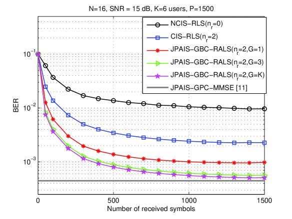
Figure 1: BER performance versus number of symbols. Parameters: $\lambda_{T}=\lambda_{k}=0.025$ (for MMSE schemes), $\alpha=0.998$, $\hat{\boldsymbol{R}}_{{\mathbf{\mathcal{S}}},k}^{-1}[i]=0.01{\boldsymbol{I}}$ and $\hat{\boldsymbol{R}}^{-1}[i]=0.01{\boldsymbol{I}}$.

The proposed JPAIS-GBC scheme is then compared with a non-cooperative approach (NCIS) and a cooperative scheme with equal power allocation (CIS) across the relays for $n_{r}=1,2$ relays. The results shown in Fig. 2 illustrate the performance improvement achieved by the JPAIS scheme and algorithms, which significantly outperform the CIS and the NCIS techniques. As the number of relays is increased so is the performance, reflecting the exploitation of the spatial diversity. In the scenario studied, the proposed JPAIS-GBC with $G=3$ can accommodate up to $3$ more users as compared to the CIS scheme and double the capacity as compared with the NCIS for the same BER performance. The curves indicate that the GBC for power allocation with only a few users is able to attain a performance close to the JPAIS-GBC with $G=K$ users, while requiring a lower complexity and less network signalling. A comprehensive study of the signalling requirements will be considered in a future work.

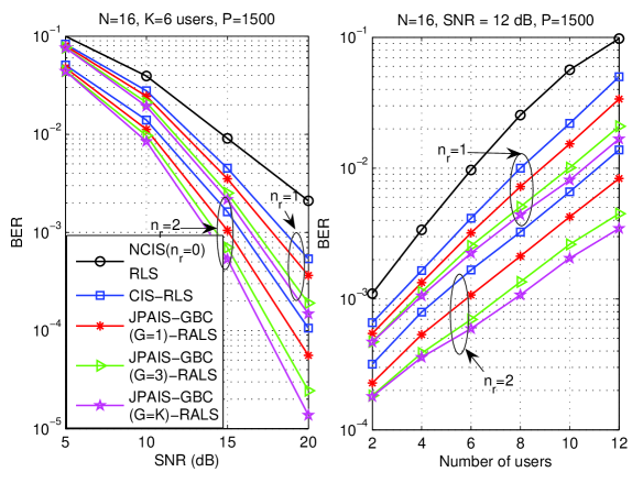
Figure 2: BER performance versus SNR and number of users for the optimal linear MMSE detectors. Parameters: $\alpha=0.998$, $\hat{\boldsymbol{R}}_{{\mathbf{\mathcal{S}}},k}^{-1}[i]=0.01{\boldsymbol{I}}$ and $\hat{\boldsymbol{R}}^{-1}[i]=0.01{\boldsymbol{I}}$.

VI Concluding Remarks

This work has proposed the JPAIS scheme with group-based constraints (GBC) for cooperative DS-CDMA networks with multiple hops and the DF protocol. A constrained MMSE design for the receive filters and the power allocation with GBC has been devised along with an MMSE channel estimator. We have proposed RALS algorithms for estimating the parameters of the channels, the receive filter and the power allocation. The results have shown that the JPAIS scheme with GBC and the RALS algorithms achieve significant gains in performance and capacity over existing schemes.

References

• [1] A. Sendonaris, E. Erkip, and B. Aazhang, โ€User cooperation diversity - Parts I and II,โ€ IEEE Trans. Commun., vol. 51, November 2003.
• [2] J. N. Laneman and G. W. Wornell, โ€Distributed space-time-coded protocols for exploiting cooperative diversity in wireless networks,โ€ IEEE Trans. Inf. Theory, vol. 49, no. 10, pp. 2415-2425, Oct. 2003.
• [3] J. N. Laneman and G. W. Wornell, โ€Cooperative diversity in wireless networks: Efficient protocols and outage behaviour,โ€ IEEE Trans. Inf. Theory, vol. 50, no. 12, pp. 3062-3080, Dec. 2004.
• [4] W. J. Huang, Y. W. Hong and C. C. J. Kuo, โ€œDecode-and-forward cooperative relay with multi-user detection in uplink CDMA networks,โ€ in Proc. IEEE GLOBECOM, November 2007, pp. 4397-4401.
• [5] G. Kramer, M. Gastpar and P. Gupta, โ€œCooperative strategies and capacity theorems for relay networks,โ€ IEEE Trans. Inf. Theory, vol. 51, no. 9, pp. 3037-3063, September 2005.
• [6] J. Luo, R. S. Blum, L. J. Cimini, L. J Greenstein, A. M. Haimovich, โ€œDecode-and-Forward Cooperative Diversity with Power Allocation in Wireless Networksโ€, IEEE Trans. Wir. Commun., vol. 6, March 2007.
• [7] L. Long and E. Hossain, โ€œCross-layer optimization frameworks for multihop wireless networks using cooperative diversityโ€œ, IEEE Trans. Wir. Commun., vol. 7, no. 7, pp. 2592-2602, July 2008.
• [8] L. Venturino, X. Wang and M. Lops, โ€œMultiuser detection for cooperative networks and performance analysis,โ€ IEEE Trans. Sig. Proc., vol. 54, no. 9, September 2006.
• [9] K. Vardhe, D. Reynolds, M. C. Valenti, โ€œThe performance of multi-user cooperative diversity in an asynchronous CDMA uplinkโ€, IEEE Trans. Wir. Commun., vol. 7, no. 5, May 2008, pp. 1930 - 1940.
• [10] R. C. de Lamare, โ€œJoint Iterative Power Allocation and Interference Suppression Algorithms for Cooperative Spread Spectrum Networksโ€, Proc. IEEE International Conference on Acoustics, Speech and Signal Processing, Dallas, USA, March 2010.
• [11] R. C. de Lamare, โ€œJoint iterative power allocation and linear interference suppression algorithms for cooperative DS-CDMA networksโ€, IET Communications, vol. 6, no. 13 , 2012, pp. 1930-1942.
• [12] J. Joung and A. H. Sayed, โ€œMultiuser two-way amplify-and-forward relay processing and power control methods for beamforming systems,โ€ IEEE Trans. on Sig. Proc., vol. 58, no. 3, pp. 1833-1846, March 2010.
• [13] M. R. Souryal, B. R. Vojcic, L. Pickholtz, โ€œAdaptive modulation in ad hoc DS/CDMA packet radio networksโ€, IEEE Trans. on Communications, vol. 54, no. 4, April 2006 pp. 714 - 725.
• [14] R. C. de Lamare, R. Sampaio-Neto, โ€œAdaptive MBER decision feedback multiuser receivers in frequency selective fading channelsโ€, IEEE Communications Letters, vol. 7, no. 2, Feb. 2003, pp. 73 - 75.
• [15] R. C. de Lamare, R. Sampaio-Neto, A. Hjorungnes, โ€œJoint iterative interference cancellation and parameter estimation for cdma systemsโ€, IEEE Communications Letters, vol. 11, no. 12, December 2007, pp. 916 - 918.
• [16] R. C. de Lamare and R. Sampaio-Neto, Minimum Mean Squared Error Iterative Successive Parallel Arbitrated Decision Feedback Detectors for DS-CDMA Systems,โ€ IEEE Transactions on Communications, vol. 56, no. 5, May 2008, pp. 778 - 789.
• [17] R. C. de Lamare and R. Sampaio-Neto, โ€œAdaptive Reduced-Rank MMSE Filtering with Interpolated FIR Filters and Adaptive Interpolatorsโ€, IEEE Sig. Proc. Letters, vol. 12, no. 3, March, 2005.
• [18] R. C. de Lamare and R. Sampaio-Neto, โ€œAdaptive Interference Suppression for DS-CDMA Systems based on Interpolated FIR Filters with Adaptive Interpolators in Multipath Channelsโ€, IEEE Transactions on Vehicular Technology, Vol. 56, no. 6, September 2007.
• [19] R. C. de Lamare and R. Sampaio-Neto, โ€œReduced-Rank Adaptive Filtering Based on Joint Iterative Optimization of Adaptive Filtersโ€, IEEE Sig. Proc. Letters, Vol. 14, no. 12, December 2007.
• [20] R. C. de Lamare and R. Sampaio-Neto, โ€œReduced-Rank Space-Time Adaptive Interference Suppression With Joint Iterative Least Squares Algorithms for Spread-Spectrum Systems,โ€ IEEE Transactions on Vehicular Technology, vol.59, no.3, March 2010, pp.1217-1228.
• [21] R. C. de Lamare and R. Sampaio-Neto, โ€œAdaptive Reduced-Rank Processing Based on Joint and Iterative Interpolation, Decimation, and Filtering,โ€ IEEE Transactions on Signal Processing, vol. 57, no. 7, July 2009, pp. 2503 - 2514.
• [22] S. Haykin, Adaptive Filter Theory, 4th ed. Englewood Cliffs, NJ: Prentice- Hall, 2002.
• [23]