Improvements to Kramers Turnover Theory

Abstract

The Kramers turnover problem, that is obtaining a uniform expression for the rate of escape of a particle over a barrier for any value of the external friction was solved in the eighties. Two formulations were given, one by Mel’nikov and Meshkov (MM) (J. Chem. Phys. 85, 1018 (1986)), which was based on a perturbation expansion for the motion of the particle in the presence of friction. The other, by Pollak, Grabert and Hänggi (PGH) (J. Chem. Phys. 91, 4073 (1989)), valid also for memory friction, was based on a perturbation expansion for the motion along the collective unstable normal mode of the particle. Both theories did not take into account the temperature dependence of the average energy loss to the bath. Increasing the bath temperature will reduce the average energy loss. In this paper, we analyse this effect, using a novel perturbation theory. We find that within the MM approach, the thermal energy gained from the bath diverges, the average energy gain becomes infinite, implying an essential failure of the theory. Within the PGH approach increasing the bath temperature reduces the average energy loss but only by a finite small amount, of the order of the inverse of the reduced barrier height. This then does not seriously affect the theory. Analysis and application for a cubic potential and Ohmic friction are presented.

I
Introduction

One of the outstanding problems of the second half of the twentieth century in rate theory was the solution for the rate of escape of a particle trapped in a potential well over an adjacent barrier whose motion is subject to a Gaussian random force and associated frictional force. In 1940, Kramers kramers40 solved this problem in two limits. In the underdamped limit, when the friction is weak he found that the rate increases linearly with increasing friction. In the opposite strong damping limit, the rate decreases inversely with the friction strength. Kramers however did not manage to derive an expression for the rate which is valid for the whole range of friction. This problem is known as the Kramers turnover problem.

An important milestone in solution of this problem was given by Mel’nikov and Meshkov (MM) in 1986 melnikov86 ; melnikov91 . They introduced into the problem the concept of a conditional probability for the particle initiated at the barrier with energy $E$ to return to it with energy $E^{\prime}$. Using perturbation theory with the friction strength as the small parameter they derived an explicit Gaussian expression for the kernel, in which the central quantity was the average energy lost by the particle to the bath as it traversed from the barrier to the well and back. This energy loss was temperature independent. Given the kernel, they wrote down a master equation for the energy flow and upon solving it were able to derive an expression for the depopulation factor rate which went smoothly from the weak damping limit where it was linear in the friction strength to unity for strong damping. They then wrote the full rate expression as a product of three terms, the ”standard” transition state theory expression for the rate, the depopulation factor, and Kramers’ spatial diffusion factor which went from unity at weak damping to being inversely proportional to the damping when the friction was strong.

Kramers’ original theory dealt with Ohmic friction, that is the white noise case. Grote and Hynes noted in the early eighties that in Chemistry one should expect the environment to have memory, since the typical time scales of a molecular surrounding are similar to that of the reacting system. They then proceeded to solve the Kramers rate problem in the presence of memory friction, in the spatial diffusion limited regime grote80 , that is in the regime of moderate to strong friction. Carmeli and Nitzan carmeli82 proceeded to do the same for the underdamped regime. However the turnover problem in the presence of memory friction remained unsolved, even after the seminal result of Mel’nikov and Meshkov.

The solution for the turnover problem, without the need for the ansatz that the rate is a product of three terms, was derived in a few steps. First, Pollak pollak86 realised in 1986 that Kramers’ problem in the spatial diffusion limit may be derived using variational transition state theory, based on a Hamiltonian description of the dynamics, in which the system is bilinearly coupled to a harmonic bath. In the vicinity of the barrier, the Hamiltonian is a quadratic form and so can be diagonalized. The normal modes then include an unstable collective mode and stable bath modes. The unstable mode is a linear combination of the system coordinate and the original (coupled) bath modes. Then Grabert grabert88 , using the discretized oscillator model derived a generalization of Mel’nikov and Meshkov’s turnover theory by considering the dynamics of the unstable normal mode, instead of the system coordinate. The continuum limit version of this theory was then derived in Ref. PGH and is known as PGH theory. Compared to Mel’nikov and Meshkov’s theory, PGH theory has two advantages: a) it is derived, there is no ansatz in the derivation; b) The result is also valid for memory friction. Practically though, the expression for the energy loss of the particle appearing in Mel’nikov and Meshkov’s theory is much simpler to implement.

Both theories ignored the fact that the average energy loss should depend on the bath temperature. As the bath temperature increases, the fluctuations increase and the bath not only dissipates energy from the system due to the frictional force, it also pumps energy back into the system. As long as the energy of the system is much higher than the thermal energy ($k_{B}T$) one expects that the particle will on the average lose energy to the bath, however as the temperature is increased the average energy lost will be reduced. This is the topic of this present paper. We will use a perturbation expansion to derive a term for the energy gained by the particle during one traversal, using the PGH approach, based on the motion of the unstable normal mode and the MM approach, based on the motion of the system coordinate. We will show that for the MM theory the average energy gain diverges, since the particle feels the fluctuations of the bath during all of its traversal. This is then an essential failure of the MM theory. For PGH theory though, to leading order in the perturbation theory the average energy loss is a sum of two parts. One is the temperature independent energy loss, due to the frictional force. The other is a fluctuation induced energy gain which grows linearly with the temperature of the bath. This energy gain is finite, since in the vicinity of the barrier the unstable mode motion decouples from the bath. Inclusion of the energy gain term in the depopulation factor is then shown to lead to a correction which is inversely proportional to the reduced barrier height, and so typically, can be neglected.

In Section II we consider the average energy loss and energy gain within PGH theory. Then in Section III we consider the average energy loss and gain within MM theory and show that for Ohmic friction, the average energy gain, at any finite temperature, diverges. In Section IV we analyse the effect of the energy gain on the depopulation factor within PGH theory. A specific analytic example for a cubic oscillator and Ohmic friction is considered in Section V. We end with a discussion of implications and further improvements of PGH theory.

II The energy loss in PGH theory

II.1 Preliminaries

The classical dynamics of the generic system is that of a particle with mass $M$ and coordinate $q$ whose classical equation of motion is a Generalized Langevin Equation (GLE) of the form:

$$M\ddot{q}+\frac{dV\left(q\right)}{dq}+M\int_{0}^{t}dt^{\prime}\gamma\left(t-t^{\prime}\right)\dot{q}\left(t^{\prime}\right)=F\left(t\right).$$ (2.1)

$F\left(t\right)$ is a Gaussian random force with zero mean and correlation function

$$\left\langle F\left(t\right)F\left(t^{\prime}\right)\right\rangle=Mk_{B}T\gamma\left(t-t^{\prime}\right).$$ (2.2)

$\gamma\left(t\right)$ is the friction function, $k_{B}$ is Boltzmann’s constant and $T$ is the temperature. The potential is assumed to have a well at $q_{a}$ with frequency $\omega_{a}$ and a barrier at $q=0$ which separates the well from either another well or a continuum. The harmonic (imaginary) frequency at the barrier top is denoted as $\omega^{{\ddagger}}$. The potential is then written as

$$V\left(q\right)=-\frac{1}{2}M\omega^{{\ddagger}2}q^{2}+V_{1}\left(q\right)$$ (2.3)

and $V_{1}\left(q\right)$ is termed the nonlinear part of the potential function. Kramers’ turnover theory provides an expression for the rate of escape of the particle from the well to the adjacent well or to the adjacent continuum as a function of the friction function, the temperature, the barrier height $V^{{\ddagger}}=V\left(0\right)-V\left(q_{a}\right)$, the mass of the particle and properties of the potential.

It is well known zwanzig73 that the GLE may be derived as the continuum limit of the equations of motion of the particle bilinearly coupled to a bath of harmonic oscillators, with mass weighted coordinates $x_{j}$ and momenta $p_{j}$:

$$H=\frac{p^{2}}{2M}+V\left(q\right)+\frac{1}{2}\sum_{j=1}^{N}\left[p_{j}^{2}+\omega_{j}^{2}\left(x_{j}-\frac{\sqrt{M}c_{j}}{\omega_{j}^{2}}q\right)^{2}\right]$$ (2.4)

where $p$ is the momentum of the particle. The friction function is identified as

$$\gamma\left(t\right)=\sum_{j=1}^{N}\frac{c_{j}^{2}}{\omega_{j}^{2}}\cos\left(\omega_{j}t\right)$$ (2.5)

and the random force is a function of the initial conditions of the bath oscillators:

$$F\left(t\right)=\sqrt{M}\sum_{j=1}^{N}c_{j}\left[\left(x_{j,0}-\frac{\sqrt{M}c_{j}q_{0}}{\omega_{j}^{2}}\right)\cos\left(\omega_{j}t\right)+\frac{p_{j,0}}{\omega_{j}}\sin\left(\omega_{j}t\right)\right].$$ (2.6)

Here, the $0$ subscript denotes the initial time. One readily finds that averaging the random force with the canonical distribution $\exp\left(-\beta H\right)$ with ($\beta=1/\left(k_{B}T\right)$) implies that it is Gaussian with zero mean and correlation function as given in Eq. 2.2.

Around the barrier top, the Hamiltonian has a quadratic form and so may be diagonalized. The details of this normal mode transformation may be found for example in Ref. liao01 . The Hamiltonian is written in terms of the system (unstable) mass weighted normal mode $\rho$ and momentum $p_{\rho}$ and stable bath normal mode coordinates $y_{j}$ and momenta $p_{y_{j}}$ as:

$$H=\frac{p_{\rho}^{2}}{2}-\frac{1}{2}\lambda^{{\ddagger}2}\rho^{2}+V_{1}\left(q\right)+\frac{1}{2}\sum_{j=1}^{N}\left[p_{y_{j}}^{2}+\lambda_{j}^{2}y_{j}^{2}\right]$$ (2.7)

with $\lambda_{j}$, the frequency of the j-th normal mode. The system coordinate $q$ is expressed in terms of the normal modes as

$$\sqrt{M}q=u_{00}\rho+\sum_{j=1}^{N}u_{j0}y_{j}$$ (2.8)

where $u_{j0}$ is the projection of the system coordinate on the j-th normal mode. The nonlinear part of the potential $V_{1}\left(q\right)$ couples the motion of the unstable normal mode $\left(\rho\right)$ motion to that of the stable normal modes ($y_{j}$). The unstable normal mode barrier frequency $\lambda^{{\ddagger}}$ is expressed in terms of the system barrier frequency and Laplace transform of the time dependent friction ($\hat{\gamma}\left(s\right)$) via the Kramers-Grote-Hynes relation kramers40 ; grote80 :

$$\lambda^{{\ddagger}2}+\hat{\gamma}\left(\lambda^{{\ddagger}}\right)\lambda^{{\ddagger}}=\omega^{{\ddagger}2}$$ (2.9)

The matrix element $u_{00}$ for the projection of the system coordinate on the unstable mode is also expressed in terms of the Laplace transform of the time dependent friction PGH :

$$u_{00}^{2}=\left[1+\frac{1}{2}\left(\frac{\hat{\gamma}\left(\lambda^{{\ddagger}}\right)}{\lambda^{{\ddagger}}}+\frac{\partial\hat{\gamma}\left(s\right)}{\partial s}|_{s=\lambda^{{\ddagger}}}\right)\right]^{-1}.$$ (2.10)

These last two relations imply that the unstable mode barrier frequency and the projection amplitude $u_{00}$ are known in the continuum limit.

The assumption of weak coupling between the system and the bath is expressed as PGH :

$$u_{1}^{2}=1-u_{00}^{2}\ll 1$$ (2.11)

which equivalently implies that the normal mode transformation elements $u_{j0},j\neq 0$ are small.

The equation of motion for each of the stable normal modes is:

$$\ddot{y}_{j}+\lambda_{j}^{2}y_{j}=-\frac{u_{j0}}{\sqrt{M}}V_{1}^{\prime}\left(\frac{1}{\sqrt{M}}\left(u_{00}\rho+\sum_{j=1}^{N}u_{j0}y_{j}\right)\right)$$ (2.12)

while the equation of motion for the unstable normal mode is:

$$\ddot{\rho}-\lambda^{{\ddagger}2}\rho=-\frac{u_{00}}{\sqrt{M}}V_{1}^{\prime}\left(\frac{1}{\sqrt{M}}\left(u_{00}\rho+\sum_{j=1}^{N}u_{j0}y_{j}\right)\right).$$ (2.13)

II.2
Perturbation theory

The motion for each of the stable bath modes may be represented in terms of a power series in the small parameter $u_{j0}$. For our purposes it suffices to consider the first two terms in such a series, so that for example the coordinate of the j-th stable mode has two components $y_{j0,t}$ and $y_{j1,t}$ of order $u_{j0}^{0}$ and $u_{j0}^{1}$ respectively. Similarly the system unstable mode motion may be expanded in a perturbation series such that the first two terms for the coordinate of the unstable mode $\rho_{0,t}$ and $\rho_{1,t}\,$ are of the order $u_{1}^{0}$ and $u_{1}^{1}$ respectively. The equations of motion for the components of each of the stable modes is

$$\ddot{y}_{j0,t}+\lambda_{j}^{2}y_{j0,t} = 0$$ (2.14)

$$\ddot{y}_{j1,t}+\lambda_{j}^{2}y_{j1,t} = -\frac{u_{j0}}{\sqrt{M}}V_{1}^{\prime}\left(\frac{u_{00}\rho_{0,t}}{\sqrt{M}}\right)$$ (2.15)

Similarly the equations of motion for the first two components of the unstable normal mode are

$$\ddot{\rho}_{0,t}-\lambda^{{\ddagger}2}\rho_{0,t}=-\frac{u_{00}}{\sqrt{M}}V_{1}^{\prime}\left(\frac{u_{00}\rho_{0,t}}{\sqrt{M}}\right)$$ (2.16)

and

$$\ddot{\rho}_{1,t}-\lambda^{{\ddagger}2}\rho_{1,t}=-\frac{u_{00}}{M}V_{1}^{\prime\prime}\left(\frac{u_{00}\rho_{0,t}}{\sqrt{M}}\right)\left(u_{00}\rho_{1,t}+\sum_{j=1}^{N}u_{j0}y_{j0,t}\right).$$ (2.17)

A central quantity in Kramers’ turnover theory is the energy gained by the bath as the unstable mode motion moves from the barrier region to the well and back. The stable mode bath energy is by definition

$$E_{B}=\frac{1}{2}\sum_{j=1}^{N}\left(p_{y_{j}}^{2}+\lambda_{j}^{2}y_{j}^{2}\right).$$ (2.18)

The change in time of the bath energy including all terms up to $u_{j0}^{2}$ is readily seen to be:

$$\frac{dE_{B}}{dt} = \sum_{j=1}^{N}\left[-\frac{u_{j0}\left(\dot{y}_{j0,t}+\dot{y}_{j1,t}\right)}{\sqrt{M}}V_{1}^{\prime}\left(\frac{u_{00}\rho_{0,t}}{\sqrt{M}}\right)-\frac{u_{j0}}{M}\dot{y}_{j0,t}\left(u_{00}\rho_{1,t}+\sum_{j=1}^{N}u_{j0}y_{j0,t}\right)V_{1}^{\prime\prime}\left(\frac{u_{00}\rho_{0,t}}{\sqrt{M}}\right)\right]$$ (2.19)

$$+O\left(u_{j0}^{3}\right)$$

so that to this order it suffices to consider only the zero-th and first order solutions for both the stable modes and the unstable mode.

The solution for the zero-th order equation of motion for the j-th stable mode is that of a harmonic oscillator

$$y_{j,0}\left(t\right)=y_{j,0}\left(t_{0}\right)\cos\left[\lambda_{j}\left(t-t_{0}\right)\right]+\frac{\dot{y}_{j,0}\left(t_{0}\right)}{\lambda_{j}}\sin\left[\lambda_{j}\left(t-t_{0}\right)\right].$$ (2.20)

It is useful to define a Gaussian random ”noise function” $\Phi\left(t\right)$ as:

$$\Phi\left(t\right)=\sum_{j=1}^{N}u_{j0}y_{j0,t}.$$ (2.21)

When averaging over the uncoupled bath Hamiltonian using the thermal distribution $\exp\left(-\beta E_{B}\left(t_{0}\right)\right)$ one readily notes that the mean of $\Phi\left(t\right)$ vanishes and the noise correlation function is

$$\left\langle\Phi\left(t\right)\Phi\left(t^{\prime}\right)\right\rangle=\frac{1}{\beta}\sum_{j=1}^{N}\frac{u_{j0}^{2}}{\lambda_{j}^{2}}\cos\left[\lambda_{j}\left(t-t^{\prime}\right)\right]\equiv\frac{1}{\beta}K\left(t-t^{\prime}\right)$$ (2.22)

and this defines the ”normal mode friction kernel” $K\left(t\right)$. Using properties of the normal mode transformation (see for example Eq. 2.17 of Ref. liao01 ) one may readily express the Laplace transform of the kernel as

$$\hat{K}\left(s\right)=\left(\frac{su_{00}^{2}}{\lambda^{{\ddagger}2}\left(s^{2}-\lambda^{{\ddagger}2}\right)}+\frac{s+\hat{\gamma}\left(s\right)}{\omega^{{\ddagger}2}\left(\omega^{{\ddagger}2}-s^{2}-\hat{\gamma}\left(s\right)s\right)}\right)$$ (2.23)

showing that it is defined in terms of the Laplace transform of the friction function and thus in the continuum limit.

The solution for the first order equation of the j-th stable mode is (taking $t_{0}\rightarrow-\infty)$:

$$y_{j1,t}=-\frac{u_{j0}}{\sqrt{M}}\int_{-\infty}^{t}dt^{\prime}\frac{\sin\left[\lambda_{j}\left(t-t^{\prime}\right)\right]}{\lambda_{j}}V_{1}^{\prime}\left(\frac{u_{00}\rho_{0,t^{\prime}}}{\sqrt{M}}\right)$$ (2.24)

and it is independent of the noise $\Phi$.

The zero-th order equation of motion for the unstable mode is that of a conservative system with a nonlinear potential. In some cases, the trajectory for the motion from the barrier top to the well and back to the barrier top is known analytically. In any case, the period of this orbit is infinite, it starts in the infinite past at the barrier and returns to it in the infinite future. Henceforth we will limit all solutions to these conditions, so that for example the initial time is taken as $-\infty$. The solution for the first order equation of motion for the unstable mode is somewhat more complex, however readily solved by using the conservation of the overall energy of the system and the bath, as shown in Appendix A. One finds that it is linear in the noise:

$$\rho_{1,t}=-\dot{\rho}_{0,t}\int_{-\infty}^{t}dt^{\prime}\frac{1}{\dot{\rho}_{0,t^{\prime}}^{2}}\int_{-\infty}^{t^{\prime}}dt^{\prime\prime}\frac{\Phi\left(t^{\prime\prime}\right)}{\sqrt{M}}\frac{d}{dt^{\prime\prime}}V_{1}^{\prime}\left(\frac{u_{00}\rho_{0,t^{\prime\prime}}}{\sqrt{M}}\right).$$ (2.25)

For later purposes, we note that the thermal average of the product of the first order solution with the time derivative of the noise is:

$$\left\langle\rho_{1,t}\dot{\Phi}\left(t\right)\right\rangle=-\frac{\dot{\rho}_{0,t}}{\sqrt{M}\beta}\int_{-\infty}^{t}dt^{\prime}\frac{1}{\dot{\rho}_{0,t^{\prime}}^{2}}\int_{-\infty}^{t^{\prime}}dt^{\prime\prime}\frac{dK\left(t-t^{\prime\prime}\right)}{dt}\frac{d}{dt^{\prime\prime}}V_{1}^{\prime}\left(\frac{u_{00}\rho_{0}\left(t^{\prime\prime}\right)}{\sqrt{M}}\right).$$ (2.26)

II.3 The thermally averaged energy loss and its variance

The thermally averaged energy loss is obtained by averaging the energy change over the thermally distributed initial conditions of the bath $\exp\left(-\beta E_{B}\left(-\infty\right)\right)$. This implies that the thermal averages of the stable mode coordinates and velocities vanish. The coordinate correlation functions are:

$$\left\langle y_{j0,t}y_{k0,t^{\prime}}\right\rangle=\frac{\cos\left[\lambda_{j}\left(t-t^{\prime}\right)\right]}{\beta\lambda_{j}^{2}}\delta_{jk}$$ (2.27)

where $\delta_{jk}$ is the Kronecker ”delta” function and from this relation one obtains by differentiation with respect to the time the velocity correlation functions. This implies for example, that $\left\langle\dot{\Phi}\left(t\right)\Phi\left(t\right)\right\rangle=0$.

The average energy loss of the system, defined as the gain in the energy of the bath as the unstable mode motion goes through one cycle, starting at the barrier and returning to it, is obtained by integration of Eq. 2.19 over the unperturbed barrier top trajectory for the unstable mode, that is the time goes from $-\infty$ to $\infty$. It is then readily found to be

$$\left\langle\Delta E\right\rangle=\int_{-\infty}^{\infty}dt\left\langle\frac{dE_{B}}{dt}\right\rangle\equiv DE_{1}-DE_{2}.$$ (2.28)

Using the first order solution for the stable mode motion (Eq. 2.24) one finds that the systematic component of the energy loss $DE_{1}$ is:

$$DE_{1}\equiv\frac{1}{2M}\int_{-\infty}^{\infty}dt\int_{-\infty}^{\infty}dt^{\prime}V_{1}^{\prime}\left(\frac{u_{00}\rho_{0,t}}{\sqrt{M}}\right)\frac{\partial^{2}K\left(t-t^{\prime}\right)}{\partial t\partial t^{\prime}}V_{1}^{\prime}\left(\frac{u_{00}\rho_{0,t^{\prime}}}{\sqrt{M}}\right)$$ (2.29)

and this is the term that also appears in PGH theory. The new result is that to the same order in the perturbation strength, there is also a temperature dependent contribution to the energy loss:

$$DE_{2}\equiv-\frac{u_{00}^{2}}{M^{2}\beta}\int_{-\infty}^{\infty}dt\int_{-\infty}^{\infty}dt^{\prime\prime}V_{1}^{\prime\prime}\left(\frac{u_{00}\rho_{0,t}}{\sqrt{M}}\right)\dot{\rho}_{0,t}\frac{dK\left(t-t^{\prime\prime}\right)}{dt}V_{1}^{\prime\prime}\left(\frac{u_{00}\rho_{0,t^{\prime\prime}}}{\sqrt{M}}\right)\dot{\rho}_{0,t^{\prime\prime}}\int_{t^{\prime\prime}}^{t}dt^{\prime}\frac{1}{\dot{\rho}_{0,t^{\prime}}^{2}}$$ (2.30)

which expresses the fact that when the bath is heated it may also transfer energy to the system. It is this temperature dependent reheating of the system which is missing in PGH theory.

The variance of the energy loss is by definition

$$\sigma^{2}=\left\langle\left(\Delta E-\left\langle\Delta E\right\rangle\right)^{2}\right\rangle.$$ (2.31)

To leading order we use only those terms which are up to quadratic in $u_{j0}$. This implies that the term $\left\langle\Delta E\right\rangle^{2}$ which is fourth order in $u_{j0}$ may be ignored. The leading order term in the energy loss is then identical to that found in PGH theory, that is:

$$\sigma^{2}=\frac{2}{\beta}DE_{1}.$$ (2.32)

III The energy loss for the system coordinate

The turnover theory of Mel’nikov and Meshkov was based on a perturbation expansion in which one considers directly the motion of the system coordinate. The small parameter is taken to be the noise $F\left(t\right)$ and we note that the friction function is second order in the noise. The system motion is separated into three parts

$$q_{t}=q_{0,t}+q_{1,t}+q_{2,t}+O\left(F^{3}\right).$$ (3.1)

which are of the order $F^{0},F^{1}$ and $F^{2}$ respectively. They obey the equations of motion:

$$0 = M\ddot{q}_{0,t}+V^{\prime}\left(q_{0,t}\right),$$ (3.2)

$$F\left(t\right) = M\ddot{q}_{1,t}+V^{\prime\prime}\left(q_{0,t}\right)q_{1,t}$$ (3.3)

$$0 = M\ddot{q}_{2,t}+V^{\prime\prime}\left(q_{0,t}\right)q_{2,t}+\frac{1}{2}V^{\left(3\right)}\left(q_{0,t}\right)q_{1,t}^{2}+M\int_{-t_{0}}^{t}dt^{\prime}\gamma\left(t-t^{\prime}\right)\dot{q}_{0,t^{\prime}}.$$ (3.4)

The time derivative of the kinetic energy of the system, including all terms up to order $F^{2}$ is then:

$$\frac{dE}{dt} = \dot{q}_{0,t}\left[-V^{\prime}\left(q_{0,t}\right)-V^{\prime\prime}\left(q_{0,t}\right)\left(q_{1,t}+q_{2,t}\right)-\frac{1}{2}V^{\left(3\right)}\left(q_{0,t}\right)q_{1,t}^{2}-M\int_{-t_{0}}^{t}dt^{\prime}\gamma\left(t-t^{\prime}\right)\dot{q}_{0,t^{\prime}}+F\left(t\right)\right]$$ (3.5)

$$+\dot{q}_{1,t}\left[-V^{\prime}\left(q_{0,t}\right)-V^{\prime\prime}\left(q_{0,t}\right)q_{1,t}+F\left(t\right)\right]-\dot{q}_{t,2}V^{\prime}\left(q_{0,t}\right)+O\left(F^{3}\right)$$

The energy loss is obtained by integrating using the zero-th order trajectory that is initiated at the barrier and returns to the barrier. Using the perturbative equations of motion given in Eqs. 3.2-3.4 one finds that to order $F^{2}$ the energy loss depends only on the zero-th and first order contributions:

$$-\Delta E_{q} = \int_{-\infty}^{\infty}dt\frac{dE}{dt}$$ (3.6)

$$= \int_{-\infty}^{\infty}dt\left[-M\dot{q}_{0,t}\int_{-\infty}^{t}dt^{\prime}\gamma\left(t-t^{\prime}\right)\dot{q}_{0,t^{\prime}}+\left(\dot{q}_{0,t}+\dot{q}_{1,t}\right)F\left(t\right)\right]+O\left(F^{3}\right).$$

Averaging over the random force then gives two contributions:

$$-\left\langle\Delta E_{q}\right\rangle=-\int_{-\infty}^{\infty}dt\left[M\dot{q}_{0,t}\int_{-\infty}^{t}dt^{\prime}\gamma\left(t-t^{\prime}\right)\dot{q}_{0,t^{\prime}}+\left\langle\dot{q}_{1,t}F\left(t\right)\right\rangle\right]+O\left(F^{3}\right).$$ (3.7)

The first contribution on the right hand side, which is independent of temperature, is the same as derived in the turnover theory of Mel’nikov and Meshkov. The second contribution is though missing.

As in the PGH approach, one may derive an explicit expression also for the second temperature dependent contribution to the energy loss. This is readily carried out using the Hamiltonian representation for the Langevin equation, as given in Eq. 2.4. For this purpose, the motion of each bath mode is also treated with perturbation theory, where the small parameter is the coupling constant $c_{j}$. The zero-th and first order contributions to the motion of the j-th bath mode are then denoted as $x_{j0,t}$ and $x_{j1,t}$ respectively. The zero-th order motion is that of the uncoupled j-th bath oscillator. The first order correction to  the j-th bath oscillator motion is readily found to be:

$$x_{j1,t}=\sqrt{M}c_{j}\int_{-\infty}^{t}dt^{\prime}\frac{\sin\left[\omega_{j}\left(t-t^{\prime}\right)\right]}{\omega_{j}}q_{0,t^{\prime}}.$$ (3.8)

Following the same derivation as in Appendix A, one notes that energy conservation implies that to first order in the coupling coefficients $c_{j}$:

$$0=\frac{p_{q,0}p_{q,1}}{M}+V^{\prime}\left(q_{0}\right)q_{1}+\sum_{j=1}^{N}\left[p_{j0}p_{j1}+\omega_{j}^{2}x_{j0}x_{j1}\right]-Fq_{0}.$$ (3.9)

This then gives a first order in time equation of motion for the first order correction to the system coordinate which is readily solved:

$$q_{1,t}=\dot{q}_{0,t}\int_{-\infty}^{t}dt^{\prime}\frac{1}{M\dot{q}_{0,t^{\prime}}^{2}}\int_{-\infty}^{t^{\prime}}dt^{\prime\prime}\dot{q}_{0,t^{\prime\prime}}F\left(t^{\prime\prime}\right)$$ (3.10)

We thus find that:

$$\left\langle\dot{q}_{1,t}F\left(t\right)\right\rangle = \frac{M}{\beta}\frac{d\ln\dot{q}_{0}}{dt}\dot{q}_{0,t}\int_{-\infty}^{t}dt^{\prime}\frac{1}{M\dot{q}_{0,t^{\prime}}^{2}}\int_{-\infty}^{t^{\prime}}dt^{\prime\prime}\dot{q}_{0,t^{\prime\prime}}\gamma\left(t-t^{\prime\prime}\right)$$ (3.11)

$$+\frac{1}{\beta\dot{q}_{0,t}}\int_{-\infty}^{t}dt^{\prime}\dot{q}_{0,t^{\prime}}\gamma\left(t-t^{\prime}\right).$$

The energy gained by the system from the bath is thus:

$$\left\langle\Delta E_{q}\right\rangle_{2} = \int_{-\infty}^{\infty}dt\left\langle\dot{q}_{t,1}F\left(t\right)\right\rangle$$ (3.12)

$$= \frac{M}{\beta}\int_{-\infty}^{\infty}dt\ddot{q}_{0,t}\int_{-\infty}^{\infty}dt^{\prime\prime}\dot{q}_{0,t^{\prime\prime}}\gamma\left(t-t^{\prime\prime}\right)\int_{t^{\prime\prime}}^{t}dt^{\prime}\frac{1}{M\dot{q}_{0,t^{\prime}}^{2}}$$

$$+\int_{-\infty}^{\infty}dt\frac{1}{\beta\dot{q}_{0,t}}\int_{-\infty}^{t}dt^{\prime}\dot{q}_{0,t^{\prime}}\gamma\left(t-t^{\prime}\right).$$

Consider then the case of Ohmic friction, that is:

$$\gamma\left(t-t^{\prime}\right)=2\gamma\delta\left(t-t^{\prime}\right)$$ (3.13)

where $\delta\left(x\right)$ is the Dirac ”delta” function. The first term on the right hand side of the second equality in Eq. 3.12 vanishes but the second term diverges:

$$\left\langle\Delta E_{q}\right\rangle_{2,Ohmic}=\frac{\gamma}{\beta}\int_{-\infty}^{\infty}dt\rightarrow\infty.$$ (3.14)

This is then an essential failure of the Mel’nikov and Meshkov solution for the turnover problem. Thermal fluctuations of the bath give an infinite amount of energy to the system. The same divergence does not occur in PGH theory where one considers the motion of the unstable normal mode. In the vicinity of the barrier, the unstable mode is decoupled from the bath and the bath can no longer affect the motion. In the Mel’nikov Meshkov theory, even arbitrarily close to the barrier top, the system coordinate remains coupled to the bath. Due to the infinite time duration of the motion, the bath can then provide an infinite amount of energy and this causes the divergence.

IV PGH turnover theory

IV.1 The energy loss conditional probability

A central object in the turnover theory is the probability kernel $P\left(E^{\prime}|E\right)$ that the system originates at the barrier with energy $E$ and returns to it with energy $E^{\prime}$. From Eq. 2.19 one readily finds that the change in energy may be written as:

$$\Delta E = E-E^{\prime}=DE_{1}+\int_{-\infty}^{\infty}dtW_{1}\left[\dot{\Phi}\left(t\right)\right]$$ (4.1)

$$+\int_{-\infty}^{\infty}dt\int_{-\infty}^{t}dt^{\prime}W_{2}\left[\dot{\Phi}\left(t\right),\Phi\left(t^{\prime}\right)\right]-\int_{-\infty}^{\infty}dtW_{3}\left[\dot{\Phi}\left(t\right),\Phi\left(t\right)\right]$$

with

$$W_{1}\left[\dot{\Phi}\left(t\right)\right] = -\frac{1}{\sqrt{M}}V_{1}^{\prime}\left(\frac{u_{00}\rho_{0}\left(t\right)}{\sqrt{M}}\right)\dot{\Phi}\left(t\right)$$ (4.2)

$$W_{2}\left[\dot{\Phi}\left(t\right),\Phi\left(t^{\prime}\right)\right] = \frac{1}{M}\dot{\Phi}\left(t\right)\frac{d}{dt}\left[V_{1}^{{}^{\prime}}\left(\frac{u_{00}\rho_{0}}{\sqrt{M}}\right)\right]\Phi\left(t^{\prime}\right)\frac{d}{dt^{\prime}}V_{1}^{\prime}\left(\frac{u_{00}\rho_{0}\left(t^{\prime}\right)}{\sqrt{M}}\right)\int_{t^{\prime}}^{t}dt^{\prime\prime}\frac{1}{\dot{\rho}_{0,t^{\prime\prime}}^{2}}$$

$$W_{3}\left[\dot{\Phi}\left(t\right),\Phi\left(t\right)\right] = \frac{\dot{\Phi}\left(t\right)\Phi\left(t\right)}{M}V_{1}^{\prime\prime}\left(\frac{u_{00}\rho_{0}}{\sqrt{M}}\right)$$ (4.4)

The thermally averaged probability $P\left(E^{\prime}|E\right)$ that the particle ends with energy $E^{\prime}$ after being initiated with energy $E$ is then by definition

$$P\left(E^{\prime}|E\right)=$$

$$\left\langle\delta\left(E^{\prime}-E+DE_{1}+\int_{-\infty}^{\infty}dt\left[W_{1}\left[\dot{\Phi}\left(t\right)\right]-W_{3}\left[\dot{\Phi}\left(t\right),\Phi\left(t\right)\right]+\int_{-\infty}^{t}dt^{\prime}W_{2}\left[\dot{\Phi}\left(t\right),\Phi\left(t^{\prime}\right)\right]\right]\right)\right\rangle_{\beta}$$

(4.5)

where the average is over the distribution

$$P\left(\text{\@text@baccent{y}},\text{\@text@baccent{p}}_{y}\right)=\prod\limits_{j=1}^{N}\frac{\beta\lambda_{j}}{2\pi}\exp\left(-\frac{\beta}{2}\left(\dot{y}_{j0}^{2}+\lambda_{j}^{2}y_{j0}^{2}\right)\right).$$ (4.6)

with $p_{y_{j}}=\dot{y}_{j}$ and we used the shortened notation $y_{j0}=y_{j,0}\left(t_{0}\right)$, etc..

If one considers only the first two terms in the energy loss (ignoring the terms with $W_{2}$ and $W_{3}$) one regains after performing the thermal averaging, the PGH kernel

$$P_{0}\left(E^{\prime}|E\right)=\left(\frac{\beta}{4\pi DE_{1}}\right)^{1/2}\exp\left(-\frac{\beta\left(E^{\prime}-E+DE_{1}\right)^{2}}{4DE_{1}}\right).$$ (4.7)

One can also explicitly perform the averaging over all modes with the full expression (including the terms with $W_{2}$ and $W_{3}$), since it involves only Gaussian integrations however we have not found a way to express the final result in the continuum limit. Instead we will consider the lowest order perturbation theory limit.

For this purpose we note that the conditional probability, to lowest order has to obey three conditions. The first is normalization, that is

$$\int_{-\infty}^{\infty}dE^{\prime}P\left(E^{\prime}|E\right)=1.$$ (4.8)

The second is that the average change in energy must be given by the average energy change found in the previous section, that is

$$\left\langle\Delta E\right\rangle=\int_{-\infty}^{\infty}dE^{\prime}P\left(E^{\prime}|E\right)\left(E-E^{\prime}\right)=DE_{1}-DE_{2}.$$ (4.9)

Thirdly, the conditional probability must obey detailed balance, that is

$$P\left(E^{\prime}|E\right)\exp\left(-\beta E\right)=P\left(E|E^{\prime}\right)\exp\left(-\beta E^{\prime}\right).$$ (4.10)

To simplify, we use henceforth the following reduced notations:

$$\varepsilon=\beta E,\text{ \ }\delta_{1}=\beta DE_{1},\text{ \ }\delta_{2}=\beta DE_{2},\text{ }y=\varepsilon^{\prime}-\varepsilon.\text{\ }$$ (4.11)

The leading order correction to the conditional probability, which also obeys detailed balance must be of the order $y^{2}$. We then write the conditional probability as:

$$P\left(\varepsilon^{\prime}|\varepsilon\right)=a\left(1-by^{2}\right)P_{0}\left(\varepsilon^{\prime}|\varepsilon\right).$$ (4.12)

The two coefficients are determined by the normalization condition and the known thermally averaged energy loss:

$$1 = \int_{-\infty}^{\infty}dya\left(1-by^{2}\right)\left(\frac{1}{4\pi\delta_{1}}\right)^{1/2}\exp\left(-\frac{\left(y+\delta_{1}\right)^{2}}{4\delta_{1}}\right)$$ (4.13)

$$\delta_{1}-\delta_{2} = -\int_{-\infty}^{\infty}dyya\left(1-by^{2}\right)\left(\frac{1}{4\pi\delta_{1}}\right)^{1/2}\exp\left(-\frac{\left(y+\delta_{1}\right)^{2}}{4\delta_{1}}\right).$$ (4.14)

One then finds that:

$$P\left(\varepsilon^{\prime}|\varepsilon\right)=\left(1+\frac{\delta_{2}}{4\delta_{1}}\left(2+\delta_{1}-\frac{y^{2}}{\delta_{1}}\right)\right)P_{0}\left(\varepsilon^{\prime}|\varepsilon\right).$$ (4.15)

IV.2
The depopulation factor

The depopulation factor given in the turnover theory is

$$\Upsilon=\exp\left(\frac{1}{2\pi}\int_{-\infty}^{\infty}d\tau\frac{\ln\left[1-\tilde{P}\left(\tau-\frac{i}{2}\right)\right]}{\tau^{2}+\frac{1}{4}}\right).$$ (4.16)

where $\tilde{P}\left(\tau-\frac{i}{2}\right)$ is the Fourier transform of the conditional probability kernel. One finds:

$$\tilde{P}\left(\tau-\frac{i}{2}\right) = \int_{-\infty}^{\infty}dy\exp\left(i(\tau-\frac{i}{2})y\right)P\left(y\right)$$ (4.17)

$$= \left(1+\delta_{2}\left(\tau^{2}+\frac{1}{4}\right)\right)\exp\left(-\delta_{1}\left(\tau^{2}+\frac{1}{4}\right)\right).$$

Assuming that the correction is small, the depopulation factor is then expanded to

$$\Upsilon\simeq\Upsilon_{0}\exp\left(-\frac{2\delta_{2}}{\delta_{1}}\left(1-\rm{erf}\left(\frac{\sqrt{\delta_{1}}}{2}\right)\right)\right)$$ (4.18)

where $\Upsilon_{0}$ is the depopulation factor using the zero-th order kernel in Eq. 4.16. One notes that the thermal correction $\delta_{2}$ reduces the depopulation factor and thus the rate. The reduced energy loss of the particle, effectively makes it more difficult to energize the particle and the rate is reduced. As we shall see considering a specific example below, the ratio $\frac{\delta_{2}}{\delta_{1}}$ is typically of the order of $1/(\beta V^{{\ddagger}})$ so that it is small and does not affect the barrier crossing rate appreciably.

V An example - Ohmic friction and escape from a cubic potential well

For Ohmic friction, the memory kernel in the normal mode representation as taken from Ref. rips90 is:

$$K\left(t\right)=\frac{u_{00}^{2}}{2\lambda^{{\ddagger}^{2}}}\left(\exp\left(-\lambda^{{\ddagger}}t\right)-\frac{\lambda^{{\ddagger}}}{\lambda_{1}}\exp\left(-\lambda_{1}t\right)+1+\frac{\lambda^{{\ddagger}}}{\lambda_{1}}\right)-\frac{1}{\omega^{{\ddagger}^{2}}}$$ (5.1)

with

$$\lambda_{1}=\left(\frac{\gamma^{2}}{4}+\omega^{{\ddagger}^{2}}\right)^{1/2}+\frac{\gamma}{2}.$$ (5.2)

For a cubic potential

$$V\left(q\right)=-\frac{M\omega^{{\ddagger}^{2}}}{2}q^{2}\left(1+\frac{q}{q_{0}}\right)$$ (5.3)

one finds rips90 that the solution for the zero-th order equation of motion for the unstable mode (Eq. 2.16) is:

$$\rho_{0,t}=-\frac{\lambda^{{\ddagger}^{2}}\sqrt{M}q_{0}}{u_{00}^{3}\omega^{{\ddagger}^{2}}\cosh^{2}\left(\frac{\lambda^{{\ddagger}}}{2}t\right)}$$ (5.4)

so that

$$DE_{2} = \frac{36}{\beta}\int_{-\infty}^{\infty}d\bar{x}\int_{0}^{\infty}d\Delta x\left(1-\exp\left(-2\Delta x\frac{\gamma}{\lambda^{{\ddagger}}}\right)\right)\exp\left(-2\Delta x\right)$$ (5.5)

$$\cdot\frac{\sinh\left(\bar{x}+\frac{\Delta x}{2}\right)}{\cosh^{5}\left(\bar{x}+\frac{\Delta x}{2}\right)}\frac{\sinh\left(\bar{x}-\frac{\Delta x}{2}\right)}{\cosh^{5}\left(\bar{x}-\frac{\Delta x}{2}\right)}\left[M\left(\bar{x}+\frac{\Delta x}{2}\right)-M\left(\bar{x}-\frac{\Delta x}{2}\right)\right]$$

where we used the notation

$$\int_{\frac{\lambda^{{\ddagger}}}{2}t^{\prime\prime}}^{\frac{\lambda^{{\ddagger}}}{2}t}dx\frac{\cosh^{6}x}{\sinh^{2}x}=M\left(\frac{\lambda^{{\ddagger}}}{2}t\right)-M\left(\frac{\lambda^{{\ddagger}}}{2}t^{\prime\prime}\right).$$ (5.6)

In the limit of weak friction $\frac{\gamma}{\lambda^{{\ddagger}}}\ll 1$ this reduces to

$$DE_{2}\left(\gamma\rightarrow 0\right)\simeq\frac{5\gamma}{\beta\omega^{{\ddagger}}}.$$ (5.7)

In this limit, the temperature independent part of the average energy loss is rips90

$$DE_{1}\left(\gamma\rightarrow 0\right)\simeq\frac{36}{5}\frac{\gamma V^{\neq}}{\omega^{{\ddagger}}}$$ (5.8)

so that the ratio of the two terms is

$$\frac{DE_{2}\left(\gamma\rightarrow 0\right)}{DE_{1}\left(\gamma\rightarrow 0\right)}\simeq\frac{25}{36\beta V^{\neq}}$$ (5.9)

which is a small number. As noted above, the temperature induced correction may be ignored in this limit.

It is also of interest to estimate the temperature dependent energy gain in the opposite limit that is when $\frac{\gamma}{\lambda^{{\ddagger}}}\simeq\frac{\gamma^{2}}{\omega^{{\ddagger}^{2}}}\gg 1$. One readily finds that

$$DE_{2}\left(\gamma\rightarrow\infty\right)\simeq\frac{5}{\beta}.$$ (5.10)

In this same limit the temperature independent energy loss is rips90

$$DE_{1}\left(\gamma\rightarrow\infty\right)=\frac{27}{35}V^{\neq}$$ (5.11)

so that:

$$\frac{DE_{2}\left(\gamma\rightarrow\infty\right)}{DE_{1}\left(\gamma\rightarrow\infty\right)}=\frac{175}{27\beta V^{\neq}}$$ (5.12)

and this is not necessarily small. Strictly speaking, in this limit the perturbation expansion is invalid, however the result does point out that when the friction is not too weak one may find discrepancies between the ”standard” PGH theory energy loss and the true energy loss, which originate from the fact that the thermal bath can also contribute to decreasing the energy loss of the system.

Figure 1: Frictional dependence of the ratio of the thermally induced energy gain (5.5) and the energy loss (2.29) for increasing barrier height (top to bottom): $\beta V^{\neq}$= 4 (dotted), 6 (short-dashed), 8 (dashed), 16 (solid).

The above results are illustrated in Figs. 1, 2 where we show the thermally induced energy gain relative to the energy loss and the reduction of the rate due to a reduction of the depopulation factor (4.16) compared to the PGH result. According to the above discussion, in the domain of low friction the ratio $DE_{2}/DE_{1}$ is mainly determined by $\beta V^{\neq}$ with the tendency to be more sensitive to dissipation for lower (reduced) barrier heights. The impact of the energy gain on the depopulation factor decreases with growing friction and increasing barrier height as indicated in (4.18): for fixed barrier height $\delta_{2}/\delta_{1}$ is almost constant while $\delta_{1}\sim\gamma V^{\neq}$ grows so that $\Upsilon/\Upsilon_{0}\to 1$. In typical experimental situations with $\beta V^{\neq}$ of the order of 10, small deviations from the PGH prediction may be found in the weak damping regime $\gamma/\omega<0.1$.

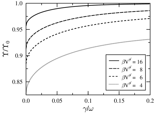
Figure 2: Ratio of the depopulation factors $\Upsilon/\Upsilon_{0}$ according to (4.16) with (4.15) and without (4.7) the thermal correction to the energy transfer kernel.

VI Discussion

The solution of the Kramers turnover problem in the 1980s has been a cornerstone result of thermal rate theory htb ; pollak05 . The rate expression obtained within PGH theory has been of practical use in a variety of fields such as chemical reactions muller08 ; muller12 and Josephson junction physics jj1 ; jj2 . However, it is incomplete as we have shown in this work since it does not include the fact that the temperature of the surrounding bath degrees of freedom will typically reduce the average energy lost by the system, due to the thermal fluctuations. Within a consistent perturbative treatment, this ”heating” contribution should be taken into account on the same footing as the dissipative part. One then finds that the thermal fluctuations indeed lead to a reduction of the energy loss that a particle experiences when traversing the well of a barrier potential. In contrast, the variance is affected only in higher order of perturbation theory. Consequently, the depopulation factor of the rate is reduced compared to the PGH prediction.

This result cannot be obtained within the Mel’nikov and Meshkov formulation where the heating contribution diverges. While the corresponding depopulation factor has often been used in practical calculations due to its simpler structure, our analysis demonstrates the inconsistency of the approach. Discrepancies between the corrected rate expression of the PGH theory and the original one are expected to be detectable in the low friction regime and in systems with moderate (reduced) barrier heights.

In this paper we have limited ourselves to the lowest order consistent contribution to the rate expression. Within the PGH framework, it is possible to go to higher order and thus obtain a further temperature dependent consistent correction also to the variance of the energy transfer. One may use the same perturbation theory to also obtain improved dynamical estimates to the rate, using the formalism of Ref. pollak93 .

Appendix A Unstable mode motion in first order

In this appendix we note that by employing energy conservation of the composite system and bath one obtains a first order in time equation of motion for the first order correction to the unstable mode motion. Using the representation of the Hamiltonian in terms of the normal modes (Eq. 2.7) one readily finds that to first order

$$p_{\rho 1,t}p_{\rho 0,t}=\lambda^{{\ddagger}2}\rho_{0,t}\rho_{1,t}-\frac{u_{00}\rho_{1,t}+\Phi\left(t\right)}{\sqrt{M}}V_{1}^{\prime}\left(\frac{u_{00}\rho_{0,t}}{\sqrt{M}}\right)-\sum_{j=1}^{N}\left[p_{y_{j1,t}}p_{y_{j0,t}}+\lambda_{j}^{2}y_{j1,t}y_{j0,t}\right].$$ (A.1)

Noting that

$$\dot{\rho}_{1,t}=p_{\rho 1,t}$$ (A.2)

we obtain a first order in time equation of motion

$$\dot{\rho}_{1,t}=\frac{d}{dt}\left[\ln\dot{\rho}_{0,t}\right]\rho_{1,t}-\frac{\Phi\left(t\right)}{\dot{\rho}_{0,t}\sqrt{M}}V_{1}^{\prime}\left(\frac{u_{00}\rho_{0,t}}{\sqrt{M}}\right)-\frac{1}{\dot{\rho}_{0,t}}\sum_{j=1}^{N}\left[p_{y_{j1,t}}p_{y_{j0,t}}+\lambda_{j}^{2}y_{j1,t}y_{j0,t}\right].$$ (A.3)

The solution for the first order correction to the motion of the stable modes has been given in Eq.  2.24. Noting that at the initial time $t_{0}$ the potential term $V_{1}\left(\frac{u_{00}\rho_{0,t}}{\sqrt{M}}\right)$ vanishes, one finds that the solution for the first order term for the unstable mode motion is:

$$\rho_{1,t}=-\dot{\rho}_{0,t}\int_{t_{0}}^{t}dt^{\prime}\frac{1}{\dot{\rho}_{0,t^{\prime}}^{2}}\int_{t_{0}}^{t^{\prime}}dt^{\prime\prime}\frac{\Phi\left(t^{\prime\prime}\right)}{\sqrt{M}}\frac{d}{dt^{\prime\prime}}V_{1}^{\prime}\left(\frac{u_{00}\rho_{0}\left(t^{\prime\prime}\right)}{\sqrt{M}}\right)$$ (A.4)

and it is linear in the noise $\Phi$. It is an instructive exercise to show by direct differentiation with respect to the time that this solution is also a solution of the second order equation of motion, as given in Eq. 2.17.

One may follow this procedure in principle to also obtain the higher order solutions. Specifically, given $\rho_{1,t}$ one obtains an explicit result for the second order contribution to the j-th stable mode $y_{j2,t}$. Then one uses again the conservation of energy to obtain a first order in time equation for $\rho_{2,t}$ which is readily solved, and so on.

References

- (1) H. A. Kramers, Physica 7, 284 (1940).
- (2) V. I. Mel’nikov and S.V. Meshkov, J. Chem. Phys. 85, 1018 (1986).
- (3) V.I. Mel’nikov, Physics Reports, 209, 1 (1991).
- (4) R.F. Grote and J.T. Hynes, J. Chem. Phys. 73, 2715 (1980).
- (5) B. Carmeli and A. Nitzan, Phys. Rev. Lett. 49, 423 (1982).
- (6) E. Pollak, J. Chem. Phys. 85, 865 (1986).
- (7) H. Grabert, Phys. Rev. Lett. 61, 1683 (1998).
- (8) E. Pollak, H. Grabert and P. Hänggi, J. Chem. Phys. 91, 4073 (1989).
- (9) R. Zwanzig, J. Stat. Phys. 9, 215 (1973).
- (10) J.L. Liao and E. Pollak, Chem. Phys. 268, 295 (2001).
- (11) I. Rips and E. Pollak, Phys. Rev. A 41, 5366 (1990).
- (12) P. Hänggi, P. Talkner and M. Borkovec, Rev. Mod. Phys. 62, 251 (1990).
- (13) E. Pollak and P. Talkner, Chaos 15, 026116 (2005).
- (14) P. L. García-Müller, F. Borondo, R. Hernandez, and R. M. Benito, Phys. Rev. Lett. 101, 178302 (2008).
- (15) P. L. García Müller, R. Hernandez, R. M. Benito, and F. Borondo, J. Chem. Phys. 137, 204301 (2012).
- (16) Q. Le Masne, H. Pothier, Norman O. Birge, C. Urbina, and D. Esteve, Phys. Rev. Lett. 102, 067002 (2009); Q. Le Masne, Thesis, University Paris 6 (2009), http://iramis.cea.fr/spec/Pres/Quantro/static/publications/phd-theses/index.html
- (17) C. Kaiser, R. Schäfer, M. Siegel, arXiv: cond-mat 1011.4241 (2011).
- (18) E. Pollak and P. Talkner, Phys. Rev. E 47, 922 (1993).