On Gaussian beams described by Jacobi’s equation

Abstract

Gaussian beams describe the amplitude and phase of rays and are widely used to model acoustic propagation. This paper describes four new results in the theory of Gaussian beams. (1) A new version of the Červený equations for the amplitude and phase of Gaussian beams is developed by applying the equivalence of Hamilton-Jacobi theory with Jacobi’s equation that connects Riemannian curvature to geodesic flow. Thus the paper makes a fundamental connection between Gaussian beams and an acoustic channel’s so-called intrinsic Gaussian curvature from differential geometry. (2) A new formula $\pi(c/c^{\prime\prime})^{1/2}$ for the distance between convergence zones is derived and applied to the Munk and other well-known profiles. (3) A class of “model spaces” are introduced that connect the acoustics of ducting/divergence zones with the channel’s Gaussian curvature ${K=cc^{\prime\prime}-(c^{\prime})^{2}}$. The model SSPs yield constant Gaussian curvature in which the geometry of ducts corresponds to great circles on a sphere and convergence zones correspond to antipodes. The distance between caustics $\pi(c/c^{\prime\prime})^{1/2}$ is equated with an ideal hyperbolic cosine SSP duct. (4) An intrinsic version of Červený’s formulae for the amplitude and phase of Gaussian beams is derived that does not depend on an extrinsic, arbitrary choice of coordinates such as range and depth. Direct comparisons are made between the computational frameworks used by the three different approaches to Gaussian beams: Snell’s law, the extrinsic Frenet-Serret formulae, and the intrinsic Jacobi methods presented here. The relationship of Gaussian beams to Riemannian curvature is explained with an overview of the modern covariant geometric methods that provide a general framework for application to other special cases.

Notation and SI Units

$t$	Time	[s]
$s$	Arclength	[m]
$T$	Ray travel-time	[s]
${\mathbf{x}}=(r,z)^{\scriptscriptstyle\rm T}$	Range and depth	[m]
$c(z)$	Sound speed profile	[m/s]
$c^{\prime}={d\over dz}c(z)$	Derivative of SSP	[1/s]
$\dot{\mathbf{x}}={d\over dt}{\mathbf{x}}$	Velocity vector	[m/s]
${\mathbf{T}}={d\over ds}{\mathbf{x}}$	Unit tangent vector	[1]
${\mathbf{N}}$	Unit normal vector	[1]
$g(\dot{\mathbf{x}},\dot{\mathbf{x}}),\ g_{ij}$	Riemannian metric	[1, $\rm s^{2}\!/m^{2}$]
$\theta_{0}$	Initial elevation angle	[rad]
$L$	Lagrangian function	[1]
$H$	Hamiltonian function	[1]
$\varkappa$	Extrinsic curvature	[1/m]
$\delta q$	Ray distance along ${\mathbf{N}}$	[m]
$\delta p=\partial T/\partial\delta q$	Conjugate momentum of $\delta q$	[s/m]
$\delta\tilde{q}=c^{-1}\,\delta q$	Travel-Time along ${\mathbf{N}}$	[s]
$\delta\tilde{p}=c\,\delta p$	Conjugate momentum of $\delta\tilde{q}$	[1]
$q=\lim{\delta q\over\delta\theta_{0}}$	Extrinsic geom. spreading	[m/rad]
$p=\lim{\delta p\over\delta\theta_{0}}$	Conj. momentum of $q$	[s/m/rad]
$\tilde{q}=c^{-1}q$	Intrinsic geom. spreading	[s/rad]
$\tilde{p}=cp$	Conjugate momentum of $\tilde{q}$	[1/rad]
${\kern 0.70004pt\raise 0.90417pt\hbox{$\ayn$}\kern 0.35002pt}=\tilde{q}$	Intrinsic geom. spreading	[s/rad]
${\kern 0.70004pt\raise 0.90417pt\hbox{$\dot{\ayn}$}\kern 0.35002pt}=(d/dt){\kern 0.70004pt\raise 0.90417pt\hbox{$\ayn$}\kern 0.35002pt}$	First derivative of	[1/rad]
$\delta t_{\rm e}={\textstyle{1\over 2}}{p\over q}\,\delta q^{2}$	Extrinsic ray tube phase	[s]
$\delta t_{\rm i}={\textstyle{1\over 2}}{{\kern 0.70004pt\raise 0.90417pt\hbox{$\dot{\ayn}$}\kern 0.35002pt}\over{\kern 0.49002pt\raise 0.63292pt\hbox{$\ayn$}\kern 0.24501pt}}\,\delta\tilde{q}^{2}$	Intrinsic ray tube phase	[s]
${\bm{T}}=\dot{\mathbf{x}}$	Ray tangent vector	[m/s]
${\bm{V}}={\kern 0.70004pt\raise 0.90417pt\hbox{$\ayn$}\kern 0.35002pt}{\bm{Y}}$	Variation vector	[m/rad]
${\bm{Y}}$	Unit parallel vector	[m/s]
$K$	Gaussian curvature	[$1/{\rm s}^{2}$]
${\bm{R}}({\bm{V}},{\bm{T}})$	Riemannian curvature	[1]
$R^{i}{}_{jkl}$	R. curvature coefficients	[$1/{\rm m}^{2}$]
$\nabla_{\bm{T}}$	Covariant differentiation	[1]
$\Gamma^{k}_{ij}$	Christoffel symbols	[1/m]

1 Introduction

This paper uses Jacobi’s equation to derive new formulae for the geometric spreading loss and phase through Gaussian beams, and thus provides an alternate method for paraxial ray tracing. [10, 9, 15, 16, 23, 24, 26, 29, 22] The new formulation, though mathematically equivalent to well-known expressions, provides new geometric insight into the physical and intrinsic geometric characteristics of Gaussian beams and their relationship to the Gaussian and Riemannian curvature of the propagation medium. Thus the expressions introduced in this paper establish the connection between Gaussian beams and the intrinsic geometry of the propagation medium. Four new geometrically-motivated ideas for ducting are presented: (1) the Červený equations for the amplitude and phase of Gaussian beams are expressed in a new form using the equivalence of the Hamilton-Jacobi equations that involves the Hamiltonian and Jacobi’s equation that involves Riemannian curvature; (2) a new formula $\pi(c/c^{\prime\prime})^{1/2}$ for the distance between convergence zones is derived, where $c(z)$ is the sound speed profile (SSP); (3) the intrinsic geometry of acoustic ducting is shown to be equivalent to great circles on a sphere with convergence zones corresponding to antipodes; (4) a coordinate-free “intrinsic” version of Červený’s formulae for the amplitude and phase of Gaussian beams is presented.

Paraxial ray methods are generally known as “Gaussian beams” because each ray is treated as representing a volume or ray tube in which the ray’s amplitude and phase in the transverse plane perpendicular to the ray’s tangent is determined by a Gaussian density. Transversely along the ray, Jacobi’s equation determines the geometric spreading loss, expressed using Riemannian or sectional curvatures, or, in the case of $2$-d rays, the Gaussian curvature. Tangentially, the relative time lag of nearby rays determines the phase of the Gaussian beam, which themselves are described by complex solutions $Ae^{j\,\varphi}$ to the Hamilton-Jacobi equations, where $A$ is the beam amplitude, $\varphi$ is the beam phase, and ${j=\sqrt{-1}}$. Therefore, the name “Gaussian beam” is highly suitable because Gaussian beams are completely determined by Gauss’s eponymous curvature.

One interesting example of a new physical insight derived from Jacobi’s equation is a simple formula for the distance between caustics: it is shown that the half-wavelength distance is about $\pi(c/c^{\prime\prime})^{1/2}$, a quantity that depends entirely on the SSP. It will be proved that the distance between convergence zones for a Munk profile with parameter $\epsilon$ and scaled depth $W$ meters is about $\pi\epsilon^{-1/2}W$ meters. For SSPs with an idealized hyperbolic cosine profile ${c(z)=c_{0}\cosh(z-z_{0})/W}$, this distance is shown to equal exactly $\pi W$ meters for all rays. Caustics arise with positive Gaussian curvature; when the curvature is negative, rays diverge and Jacobi’s equation quantifies their divergence, or transmission loss. For example, for linear SSPs with slope $c^{\prime}$ the geometric spreading at time ${t\lessapprox c^{\prime-1}}$ is about ${ct+{1\over 6}c(c^{\prime})^{2}t^{3}}$. These results are both a direct consequence of the fact that the Gaussian curvature of the propagation medium equals ${K=cc^{\prime\prime}-(c^{\prime})^{2}}$. Classifying the SSP by its Gaussian curvature will allow for the introduction of model spaces for convergent ducts whose curvature is constant positive, divergence zones with constant negative curvature, and simple non-refractive spreading with vanishing curvature. Another feature arising from this work is an accounting of the additional spreading loss for either reflected or transmitted rays at an interface, at which point the Gaussian curvature is not defined.

Direct comparisons are made between the computational frameworks derived from the three different approaches to Gaussian beams: (1) Snell’s law, [11, 27, 12, 13, 18, 22, 38] (2) a variant of the extrinsic Frenet-Serret established by Červený and colleagues, [15, 16] and (3) the new intrinsic methods presented here. Bergman, [6, 7, 8] apparently the first to recognize the application of Jacobi’s equation to ray tracing, recently adopted methods from General Relativity to address the problem of computing ray amplitudes in a relativistic acoustic field. The non-relativistic intrinsic results developed in this paper are equivalent to many of Bergman’s if one uses the space-like part of his pseudo-Riemannian Lorentz metric.

It is perhaps noteworthy that Jacobi’s equation and its full implications for Gaussian beams has, apparently, not yet appeared in the acoustical literature. This lacuna might be defended by a few historical observations. Lord Rayleigh was initially dismissive of the practical applications for acoustic refraction, noting in 1877 “almost the only instance of acoustical refraction, which has practical interest, is the deviation of sonorous rays from rectilinear course due to the heterogeneity of the atmosphere.” [31] Though the foundations of non-Euclidean geometry had been established by this time, differential and Riemannian geometry remains relatively little known in engineering applications to this day, in spite of the fact that covariant analysis is the natural approach to many physical and engineering problems, as will be seen in its application to Gaussian beams here.

In section 2 the ray equations developed using the classical Euler-Lagrange, Frenet-Serret, and Hamilton-Jacobi formulations, followed by the amplitude and phase along a specific ray using Červený’s Hamilton-Jacobi approach. This standard development is then recast using an intrinsic parameterization that will be shown equivalent to Jacobi’s equation. Section 3 develops an intrinsic formulation of Gaussian beams based on Jacobi’s equation and explores the physical consequences of this approach, including a computation of the distance between convergence zones and a classification of SSPs using “model spaces” of constant Gaussian curvature.

2 Gaussian Beams in Horizontally Stratified Isotropic Media

The simplest and most frequently encountered case of acoustic rays in a horizontally stratified isotropic medium will be analyzed. As usual, denote the three spatial coordinates by the variables $x$, $y$, and $z$, time by $t$, the spatial infinitesimal arclength by $ds^{2}=dx^{2}+dy^{2}+dz^{2}$, and the depth-dependent SSP by $c(z)$, differentiable except at a discrete set of points where either $c(z)$ itself is discontinuous (e.g. Snell’s law), or its first derivative $c^{\prime}(z)=dc/dz$ is discontinuous (e.g. method of images at a boundary). Paths ${\mathbf{x}}(t)=\bigl{(}r(t),\phi(t),z(t)\bigr{)}^{\scriptscriptstyle\rm T}$ are expressed using cylindrical coordinates, with $r=\sqrt{\mathstrut x^{2}+y^{2}}$, $\phi={\tan^{-1}(y/x)}$, and $z$ (pointing down), so that $ds^{2}=dr^{2}+r^{2}\,d\phi^{2}+dz^{2}$. The physical solution is independent of these coordinates. The time required to travel along an arbitrary continuous path equals

$$T[{\mathbf{x}}(t)]=\int dt=\int{1\over c(z)}{ds\over dt}dt=\int c^{-1}(z)(\dot{r}^{2}+r^{2}\dot{\phi}^{2}+\dot{z}^{2})^{1/2}\,dt.$$ (1)

where $\dot{\mathbf{x}}(t)=d{\mathbf{x}}/dt$ and ${ds/dt=c(z)}$. The Fermat metric is represented by the quadratic function $g(\dot{\mathbf{x}},\dot{\mathbf{x}})=c^{-2}(z)(\dot{r}^{2}+r^{2}\dot{\phi}^{2}+\dot{z}^{2})$, whose square-root appears in Eq. (1). This Riemannian metric has coefficients ${{\mathbf{G}}=(g_{ij})}$ and induces an inner product $\langle\dot{\mathbf{x}},\dot{\mathbf{y}}\rangle=g(\dot{\mathbf{x}},\dot{\mathbf{y}})=c^{-2}(z)(\dot{r}_{1}\dot{r}_{2}+r^{2}\dot{\phi}_{1}\dot{\phi}_{2}+\dot{z}_{1}\dot{z}_{2})$ and norm $\|\dot{\mathbf{x}}\|^{2}=g(\dot{\mathbf{x}},\dot{\mathbf{x}})$ on the space of tangent vectors $(\dot{r},\dot{\phi},\dot{z})^{\scriptscriptstyle\rm T}$ at each point $(r,\phi,z)^{\scriptscriptstyle\rm T}$.

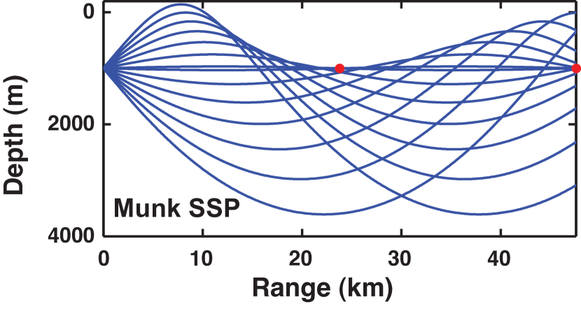
Fig. 1: Rays for the Munk SSP [22] with with parameter ${\epsilon=0.00737}$, scaled depth ${\bar{z}=(z-z_{0})/W}$ with ${W=650\,}$m, and (nonconstant) Gaussian curvature ${K=\epsilon c_{0}^{2}/W^{2}}$ at $z_{0}$, yielding convergence zones at about every ${\pi\epsilon^{-1/2}W=23.8\,}$km (Theorem 6) as illustrated by the red dots ($\bullet$). The rays are computed using a standard 4th order Runge-Kutta ODE solver.

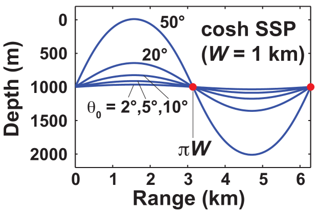
Fig. 2: Rays for the hyperbolic cosine SSP $c(z)=c_{0}\cosh({z-z_{0}})/W$ with $z_{0}=W=1\,$km. This SSP yields a space of constant positive curvature, resulting in a duct with convergent rays and caustics independent of any initial elevation angle $\theta_{0}$ at ranges ${\pi W=3.14159}\ldots\,$km (Theorem 7), illustrated by the red dots ($\bullet$). The rays are computed using a standard 4th order Runge-Kutta ODE solver.

Before the main results of the paper involving the geometry of acoustic ducting and divergence are presented, a concise background of ray theory is provided in Subsections 2.1 and 2.2 using the Euler-Lagrange, Frenet-Serret, and Hamilton-Jacobi formulations. Subsection 2.3 derives the amplitude and phase along a specific ray using Červený’s Hamilton-Jacobi approach. Červený’s equations are recast in section 2.4 using an intrinsic parameterization that will be shown in section 3 to yield Jacobi’s equation expressed in form that yields geometric insight into acoustic ducting.

2.1 Ray Equations: Euler-Lagrange and Frenet-Serret

Fermat’s principle implies that rays satisfy the Euler-Lagrange equation, ${(d/dt)(\partial L/\partial\dot{\mathbf{x}})-(\partial L/\partial{\mathbf{x}})}={\bm{0}}$, with either initial conditions or boundary conditions for eigenrays. Attention is restricted to the $(r,z)$-plane because radial symmetry implies that $\phi(t)\equiv\phi_{0}$. The Euler-Lagrange equations with Lagrangian $L(t;r,z;\dot{r},\dot{z})=c^{-1}(z)(\dot{r}^{2}+\dot{z}^{2})^{1/2}$ and radial symmetry ${\dot{\phi}\equiv 0}$ yields the well-known differential ray (Christoffel) equations

$$\ddot{r}-2(c^{\prime}/c)\dot{r}\dot{z}=0,\qquad\ddot{z}+(c^{\prime}/c)(\dot{r}^{2}-\dot{z}^{2})=0.$$ (2)

Figs. 1 and 2 illustrate computed rays determined by the Munk and hyperbolic cosine SSPs. Parameterization by travel-time $t$ is said to be “natural” or “intrinsic” because rays minimize travel-time. It is oftentimes computationally convenient to parameterize rays by “extrinsic” arclength $ds=({dr^{2}+dz^{2}})^{1/2}$, in which case Eq. (2) becomes the first Frenet-Serret formula $(d^{2}/ds^{2})(r,z)^{\scriptscriptstyle\rm T}=(c^{\prime}/c)(dr/ds)(dz/ds,-dr/ds)^{\scriptscriptstyle\rm T}$, i.e. $d{\mathbf{T}}/ds=\varkappa{\mathbf{N}}$, where ${\mathbf{T}}=(dr/ds,dz/ds)^{\scriptscriptstyle\rm T}$ is the ray’s tangent vector, ${\mathbf{N}}=(dz/ds,-dr/ds)^{\scriptscriptstyle\rm T}$ is its normal (always defined in the same direction), and $\varkappa=(c^{\prime}/c)\*(dr/ds)=-c_{\rm n}/c$ is the ray’s extrinsic curvature, and $c_{\rm n}=(\partial c/\partial{\mathbf{x}}){\cdot}{\mathbf{N}}=-c^{\prime}(dr/ds)$ is the first derivative of the SSP $c$ in the normal direction. The quadratic coefficients for the tangent vector (first derivative) terms that appear in the ray equations [Eq. (2)] are called Christoffel symbols of the second kind, [17, 20, 32, 34] and are crucial in quantifying the amplitude and phase along the ray caused by geometric spreading. A continuous version of Snell’s law [11, 13, 18, 22, 38] yields the integral solution

$$r(z;\theta_{0})=\int_{z_{0}}^{z}{ac(z_{\prime})\over\bigl{(}1-a^{2}c^{2}(z_{\prime})\bigr{)}^{1/2}}\,dz_{\prime},$$ (3)

in which ${a=c^{-1}(z_{0})\cos\theta_{0}}$ is the Snell invariant with initial conditions $\bigl{(}r(0),z(0)\bigr{)}=(0,z_{0})$ and $\bigl{(}\dot{r}(0),\dot{z}(0)\bigr{)}=c(z_{0})(\cos\theta_{0},-\sin\theta_{0})$.

2.2 Ray Equations: Hamilton-Jacobi Equation

Rays satisfy the canonical form of the Euler-Lagrange equations ${z^{\prime}=\partial H/\partial\zeta}$, ${\zeta^{\prime}=-\partial H/\partial z}$ with Hamiltonian $H(r;z;\zeta)=\zeta z^{\prime}-L(r;z;z^{\prime})$ and $\zeta=\partial L/\partial z^{\prime}$. The travel-time $T$ of Eq. (1) satisfies the Hamilton-Jacobi equation $(\partial T/\partial r)+H(r;z;\partial T/\partial z)=0$, which reduces to the well-known eikonal equation $(\partial T/\partial r)^{2}+(\partial T/\partial z)^{2}=c^{-2}(z)$ for the Hamiltonian $H(r;z;\zeta)=-\bigl{(}c^{-2}(z)-\zeta^{2}\bigr{)}^{1/2}$ corresponding to the Lagrangian in section 2.1.

2.3 Paraxial Ray Equations: Hamilton-Jacobi Form

Ray amplitude is determined by the spreading of nearby rays, and phase away from the ray is determined by time differences, so that rays are viewed as tubes or beams possessing both amplitude and phase rather than the skeletal objects determined by Eq. (2). As first established by Červený and colleagues, [15, 16, 23, 29, 22] the equations for the amplitude and phase along a ray tube are given by the canonical equations after a convenient change of variables involving the ray itself. Let $s$ be the arclength along the ray and let $\delta q$ be the small or infinitesimal distance away from the ray, measured perpendicularly along the normal ${\mathbf{N}}$ at arclength $s$ such that

$$\begin{pmatrix}r(s,\delta q)\\ z(s,\delta q)\end{pmatrix}=\begin{pmatrix}r(s)\\ z(s)\end{pmatrix}+\delta q\begin{pmatrix}dz/ds\\ -dr/ds\end{pmatrix},$$ (4)

and let

$$\delta p=\partial T/\partial\delta q$$ (5)

be the small or infinitesimal derivative of travel-time w.r.t. $\delta q$ from the ray along the line ${\mathbf{N}}$, all illustrated in Fig. 3. Thus, $\delta q$ quantifies the spread of nearby rays, and therefore determines the ray’s amplitude, and as shown by Červený [16] the conjugate momentum $\delta p$ appears in the difference in time-of-travel nearby rays along ${\mathbf{N}}$ and thus determines the ray’s phase. Following Červený [16] (also see Wolf and Krötzsch [39]) Hamilton-Jacobi theory is used to determine the governing equations for $\delta q$ and $\delta p$.

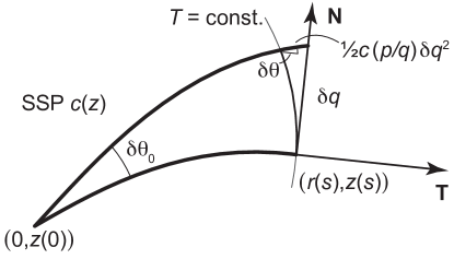
Fig. 3: Ray tube in a horizontally stratified medium. The azimuthal component, not shown, is perpendicular to the page. All distances in the figure represent actual, extrinsic Euclidean distance. The extrinsic distance between nearby rays along the normal vector ${\mathbf{N}}$ is denoted as $\delta q$, and the nearby ray’s additional length equals ${1\over 2}c(\delta p/\delta q)\,\delta q^{2}={1\over 2}c(p/q)\,\delta q^{2}$, where $q=\lim\delta q/\delta\theta_{0}$ is the extrinsic geometric spreading, and $\delta p=\partial T/\partial\delta q$ and $p=\partial T/\partial q$ are the conjugate momenta corresponding to $\delta q$ and $q$.

By the chain rule $\partial T/\partial(s,\delta q)=\partial T/\partial(r,z){\cdot}J$, where $J=\partial(r,z)/\partial(s,\delta q)=\bigl{(}h{\mathbf{T}},{\mathbf{N}}\bigr{)}$ is the Jacobian matrix along the ray at distance $s$ at ${\delta q=0}$ with scale factor $h(s,\delta q)=1-\bigl{(}(c^{\prime}/c)(dr/ds)\bigr{)}|_{\delta q=0}\,\delta q=1+(c_{\rm n}/c)|_{\delta q=0}\,\delta q$. The eikonal equation expressed in the ray-centered coordinates $s$ and $\delta q$ is $h^{-2}(s,\delta q)(\partial T/\partial s)^{2}+(\partial T/\partial\delta q)^{2}=c^{-2}(s,\delta q)$, corresponding to the Hamiltonian $H(s;\delta q;\delta p)=-h(s,\delta q)\*\bigl{(}{c^{-2}(s,\delta q)-\delta p^{2}}\bigr{)}^{1/2}$. For small $\delta q$ and $\delta p$ up to second-order,

$${1\over c(s,\delta q)} = {1\over c_{s}}-{c_{\rm n}\over c_{s}^{2}}\,\delta q-{1\over 2}\left({c_{\rm nn}\over c_{s}^{2}}-2{c_{\rm n}^{2}\over c_{s}^{3}}\right)\,\delta q^{2}+\cdots,$$ (6)

$$H(s;\delta q;\delta p) = -hc^{-1}(s,\delta q)(1-{\textstyle{1\over 2}}c_{s}^{2}\,\delta p^{2})+\cdots$$ (7)

$$\quad{}=-c_{s}^{-1}+{c_{\rm nn}\over 2c_{s}^{2}}\,\delta q^{2}+{1\over 2}c_{s}\,\delta p^{2}+\cdots$$, (8)

where $c_{s}=c\bigl{(}z(s)\bigr{)}$ and $c_{\rm nn}=c^{\prime\prime}\bigl{(}z(s)\bigr{)}(dr/ds)^{2}$ is the second derivative of the SSP in the direction of the ray normal.

Applying Hamilton’s equations of motion ${d\delta q/ds=\partial H/\partial\delta p}$, ${d\delta p/ds=-\partial H/\partial\delta q}$ to Eq. (8) yields the paraxial ray tracing equations, a system of ordinary differential equations [10, 15, 16, 22, 23, 24, 26, 29, 33]

the initial conditions arising from the facts that the spread of rays separated by a small angle $\delta\theta_{0}$ is zero at ${s=0}$, and the differential time equals ${\delta T=c_{0}^{-1}\,\delta q\,\delta\theta_{0}}$.

2.4 Paraxial Ray Equations: Sturm-Liouville Form

Before explaining the full significance of the complete second-order terms in the paraxial ray equations in the next section, it will be helpful to express Eqs. (LABEL:eq:delqde)–(LABEL:eq:delpde) as a single second-order differential equation using the natural or intrinsic parameters of the problem. Consistent with much of existing literature on paraxial rays, rays are parameterize using the arclength $s$. However, physically rays do not minimize arclength, but travel-time $t$, and therefore the paraxial ray’s underlying physical and geometric properties will be revealed by using the intrinsic parameterization $dt=c^{-1}\,ds$. Also the variables $\delta q$ and $\delta p=\partial T/\partial\delta q$ are expressed using arclength or distance; the corresponding intrinsic variables arise by converting distance $\delta q$ to travel-time $\delta\tilde{q}$ and slowness $\delta p$ to the dimensionless $\delta\tilde{p}$ using the sound speed $c$:

$$\delta\tilde{q}\buildrel\rm def\over{=}c^{-1}\,\delta q,\quad\hbox{and}\quad\delta\tilde{p}\buildrel\rm def\over{=}c\,\delta p.$$ (10)

Note that $\delta\tilde{q}$ is the travel-time between nearby rays and $\delta\tilde{p}=\partial T/\partial\delta\tilde{q}$ is the travel-time derivative along a straight-line path normal. The geometric significance of these intrinsic coordinates is made clear by the following new theorem:

Theorem 1.

Let $\delta q$ and $\delta p$ satisfy Eqs. (LABEL:eq:delqde)–(LABEL:eq:delpde). Then these extrinsic first-order paraxial ray equations are equivalent to the intrinsic second-order paraxial ray equation

$$\delta\ddot{\tilde{q}}+\bigl{(}cc^{\prime\prime}-(c^{\prime})^{2}\bigr{)}\,\delta\tilde{q}=0,$$ (11)

where $\delta\tilde{q}=c^{-1}\,\delta q$, $\delta\tilde{p}=c\,\delta p$, $\delta\ddot{\tilde{q}}=(d^{2}/dt^{2})\delta\tilde{q}$, and the coefficient ${cc^{\prime\prime}-(c^{\prime})^{2}}$ is the Gaussian curvature of the propagation medium w.r.t. to the Fermat metric of Eq. (1).

The proof involves parameterizing by travel-time $t$ and expressing the Hamilton form of the paraxial ray equations of Eqs. (LABEL:eq:delqde)–(LABEL:eq:delpde) as the coupled first-order system,

Taking another derivative of the first equation yields ${\delta\ddot{\tilde{q}}+K\,\delta\tilde{q}=0}$ with $K={cc^{\prime\prime}-(c^{\prime})^{2}}$. The theorem is thus proven by demonstrating that this expression for $K$ is precisely the Gaussian curvature w.r.t. the Fermat metric of Eq. (1). Given an arbitrary metric $g$ on a $2$-dimensional manifold with coefficients ${g_{ij}=g({\bm{X}}_{i},{\bm{X}}_{j})}$ w.r.t. a basis $\{\,{\bm{X}}_{i}\,\}$, the Gaussian curvature is determined [32, 34] by the expression $K=R_{1212}/({g_{11}g_{22}-g_{12}^{2}})$ in which $R_{ijkl}=\sum_{n}g_{in}R^{n}{}_{jkl}$, $R^{i}{}_{jkl}=(\partial\Gamma^{i}_{lj}/\partial x^{k})-(\partial\Gamma^{i}_{kj}/\partial x^{l})+\sum\nolimits_{n}({\Gamma^{n}_{lj}\Gamma^{i}_{kn}-\Gamma^{n}_{kj}\Gamma^{i}_{ln}})$ are the coefficients of the Riemannian curvature tensor ${\bm{R}}$, and the Christoffel symbols (of the second kind) $\Gamma^{k}_{ij}={1\over 2}\sum\nolimits_{l}g^{kl}\bigl{(}(\partial g_{il}/\partial x^{j})+(\partial g_{jl}/\partial x^{i})-(\partial g_{ij}/\partial x^{l})\bigr{)}$ appear in the quadratic coefficients in the ray (geodesic) equations

$$\textstyle\ddot{x}^{k}+\sum\nolimits_{ij}\Gamma^{k}_{ij}\dot{x}^{i}\dot{x}^{j}=0$$ (13)

with ${(g^{kl})=(g_{ij})^{-1}}$ representing the matrix inverse of the matrix of metric coefficients. [20, 32, 34] The Christoffel symbols expressed as quadratic forms are

$$(\Gamma^{1}_{ij})=\begin{pmatrix}0&-c^{\prime}/c\\ -c^{\prime}/c&0\end{pmatrix},\quad(\Gamma^{2}_{ij})=\begin{pmatrix}c^{\prime}/c&0\\ 0&-c^{\prime}/c\end{pmatrix},$$ (14)

can be read directly from the ray equations of Eq. (2); these along with the matrix $(g_{ij})=c^{-2}\Bigl{(}{1\atop 0}\;{0\atop 1}\Bigr{)}$ can be used directly with the preceding equations to compute the Gaussian curvature ${K=cc^{\prime\prime}-(c^{\prime})^{2}}$. As will be proved, Eq. (11) is precisely Jacobi’s equation; therefore, the Hamiltonian form of the paraxial ray equations (LABEL:eq:delqde)–(LABEL:eq:delpde) is mathematically and physically equivalent to the intrinsic Jacobi’s equation. This equivalence between Červený’s formulation of Gaussian beams and Jacobi’s equation is a new result. The functional form of the Gaussian curvature will be used to derive the distance between convergence zones and “model spaces” of constant curvature for the SSP.

3 Intrinsic Geometry of Gaussian Beams

3.1 Transverse Amplitude of a Gaussian Beam

This section contains an analysis of Gaussian beams that use Jacobi’s equation to quantify their amplitude and phase. All the results obtained so far have been for rays and infinitesimal variations around them. In contrast, Gaussian beams have real, finite physical width that must be accounted for in the plane transverse to the ray. The physical width has different implications for the Gaussian beam’s amplitude and phase. The amplitude is determined by both the geometric spreading loss along the ray and the initial amplitude distribution in the transverse plane. The phase is determined by the differential change in travel-time along the transverse plane. Mathematically, the scaled normal vector $\delta q\,{\mathbf{N}}$ represents the infinitesimal change in ray position as a function of the take-off angle for a fixed path length $s$. Gauss’s lemma implies that this travel-time is fixed to first-order, but says nothing about the second-order terms, i.e. ${\mathbf{x}}(s;\theta_{0})+\delta q{\mathbf{N}}={\mathbf{x}}(s;{\theta_{0}+\delta\theta_{0}})+O(\delta\theta_{0}^{2})$ for ${\delta\theta_{0}>0}$. This ray-front curvature effect is seen in Euclidean space by holding a ruler next to a circle or cylinder and observing the size of gap—which for a circle of radius $R$ has a gap size of ${R\sec\delta\theta-R}={(R/2)\delta\theta^{2}+O(\delta\theta^{4})}$. The second-order travel-time difference is often physically significant because it is of the order of several wavelengths at a broad range of frequencies $f_{0}$ and therefore does contribute to the Gaussian beam’s phase $2\pi f_{0}t$. Because the travel-time difference in the transverse plane is quadratic, the phase of Gaussian beam necessarily has a Gaussian distribution. Furthermore, these second-order affects are already accounted for in the Riemannian curvature terms determining the Gaussian beam’s amplitude, so the Gaussian beam’s amplitude in the transverse plane is determined by the effect of geometric spreading on initial conditions. In this subsection we will quantify the impact of the initial conditions on the amplitude and the second-order travel-time differences on the phase. Both quantities are determined by the ray distance $\delta q$, which will now be formalized for both extrinsic and intrinsic geometric spreading.

Definition 2.

(Geometric spreading) Let ${\mathbf{x}}(s;\theta_{0})=\bigl{(}r(s;\theta_{0}),z(s;\theta_{0})\bigr{)}^{\scriptscriptstyle\rm T}$ be a ray parameterized by arclength $s$ with initial conditions ${\mathbf{x}}(0;\theta_{0})=(0,z_{0})^{\scriptscriptstyle\rm T}$ and $(d/ds){\mathbf{x}}(0;\theta_{0})=(\cos\theta_{0},-\sin\theta_{0})^{\scriptscriptstyle\rm T}$ in a horizontally stratified media with SSP $c(z)$. The extrinsic geometric spreading $q(s)$ along the ray caused by a change in elevation angle $\theta_{0}$ is defined to be

$$q(s)=\|(\partial{\mathbf{x}}(s;\theta_{0})/\partial\theta_{0})_{s}\|_{2},$$ (15)

where $\|{\cdot}\|_{2}$ denotes the standard $2$-norm and the standard notation $(\partial/\partial\theta_{0})_{s}$ means partial differentiation w.r.t. $\theta_{0}$ while holding arclength $s$ constant.

Theorem 3.

(Geometric spreading for horizontally stratified media [22]) Let ${\mathbf{x}}(s)=\bigl{(}r(s;\theta_{0}),z(s;\theta_{0})\bigr{)}^{\scriptscriptstyle\rm T}$ be a ray in a horizontally stratified medium with a twice-differentiable SSP $c(z)$ parameterized by arclength $s$ and with initial elevation angle $\theta_{0}$. The extrinsic geometric spreading $q$ and the corresponding canonical variable $p=\partial T/\partial q$ along the ray are determined by

$$q=\lim_{\delta\theta_{0}\to 0}\delta q/\delta\theta_{0},\qquad p=\lim_{\delta\theta_{0}\to 0}\delta p/\delta\theta_{0},$$ (16)

and satisfy the Hamilton equations

The proof is a trivial application of the definition of the small or infinitesimal difference $\delta q$ defined in Eq. (4). The theorem follows immediately by dividing Eqs. (LABEL:eq:delqde)–(LABEL:eq:delpde) by $\delta\theta_{0}$ and taking the limit. Thus we have a complete description of the extrinsic geometric spreading for Gaussian beams, including the complete second-order terms introduced in Eq. (LABEL:eq:delpde). To appreciate the geometric significance of the spread, we will define the intrinsic geometric spreading and equate this concept with Jacobi’s equation first encountered in Theorem 1, expressed in this new theorem:

Definition 4.

(Intrinsic geometric spreading for horizontally stratified media) Let ${\bigl{(}r(t;\theta_{0}),z(t;\theta_{0})\bigr{)}}$ be a ray in a horizontally stratified medium with a twice-differentiable SSP $c(z)$ as in Theorem 3, but parameterized by path time $t$. The intrinsic geometric spreading ${\kern 1.00006pt\raise 1.29167pt\hbox{$\ayn$}\kern 0.50003pt}(t)$ along the ray is defined to be

$${\kern 1.00006pt\raise 1.29167pt\hbox{$\ayn$}\kern 0.50003pt}(t)=\lim_{\delta\theta_{0}\to 0}{\delta\tilde{q}\over\delta\theta_{0}}=c^{-1}q(t)=\tilde{q}(t),$$ (18)

where $\delta\tilde{q}$ is the travel-time between nearby rays separated by $\delta\theta_{0}$ at their initial point defined in Eq. (10), and $q(t)$ is the extrinsic geometric spreading parameterized by time. [Intrinsic geometric spreading is denoted by the Arabic letter ‘ayn, (‘’, pronounced like the end of ‘nine’ spoken with a strong Australian accent) in recognition of the mathematician Ibn Sahl who discovered Snell’s law of refraction around 984. Ibn Sahl used the symbol  to denote the center of a lens [30].]

The intrinsic geometric spreading is a consequence of an obvious corollary to Theorem 3 arising from Eqs. (LABEL:eq:tildeqde)–(LABEL:eq:tildepde) for the intrinsic variables

$$\tilde{q}=c^{-1}q=\lim_{\delta\theta_{0}\to 0}\delta\tilde{q}/\delta\theta_{0}={\kern 1.00006pt\raise 1.29167pt\hbox{$\ayn$}\kern 0.50003pt},\quad\hbox{and}\quad\tilde{p}=cp=\lim_{\delta\theta_{0}\to 0}\delta\tilde{p}/\delta\theta_{0}={\kern 1.00006pt\raise 1.29167pt\hbox{$\dot{\ayn}$}\kern 0.50003pt}+c^{\prime}\sin\theta{\kern 1.00006pt\raise 1.29167pt\hbox{$\ayn$}\kern 0.50003pt}.$$ (19)

Note that the path time derivative ${\tilde{p}=\partial T/\partial\tilde{q}}$ w.r.t. distances along the extrinsic path normal ${\mathbf{N}}$ is not exactly equal to the derivative ${\kern 1.00006pt\raise 1.29167pt\hbox{$\dot{\ayn}$}\kern 0.50003pt}=(d/dt){\kern 1.00006pt\raise 1.29167pt\hbox{$\ayn$}\kern 0.50003pt}$ of the intrinsic geometric spreading; the geometric reason for this difference will be explained in section 3.7. We are now ready to introduce Jacobi’s equation and thereby compute the ray’s amplitude determined by the geometric spreading, as well a Gaussian beam’s phase in the transverse plane perpendicular to the ray’s tangent.

Theorem 5.

(Intrinsic geometric spreading for horizontally stratified media) Let ${\bigl{(}r(t;\theta_{0}),z(t;\theta_{0})\bigr{)}^{\scriptscriptstyle\rm T}}$ be a ray in a horizontally stratified medium with a twice-differentiable SSP $c(z)$ parameterized by path time $t$ and with initial elevation angle $\theta_{0}$. The intrinsic geometric spreading ${\kern 1.00006pt\raise 1.29167pt\hbox{$\ayn$}\kern 0.50003pt}(t)$ along the ray satisfies the Sturm-Liouville equation

$$\ddot{\kern 1.00006pt\raise 1.29167pt\hbox{$\ayn$}\kern 0.50003pt}+K(t){\kern 1.00006pt\raise 1.29167pt\hbox{$\ayn$}\kern 0.50003pt}=0;\quad{\kern 1.00006pt\raise 1.29167pt\hbox{$\ayn$}\kern 0.50003pt}(0)=0,\ {\kern 1.00006pt\raise 1.29167pt\hbox{$\dot{\ayn}$}\kern 0.50003pt}(0)=1,$$ (20)

where

$$K=cc^{\prime\prime}-(c^{\prime})^{2}$$ (21)

is the acoustic Gaussian curvature of the Fermat metric $g(\dot{\mathbf{x}},\dot{\mathbf{x}})=c^{-2}(z)(\dot{r}^{2}+\dot{z}^{2})$ of Eq. (1).

Eq. (20) is simply the intrinsic Jacobi’s equation in two dimensions encountered above in Eq. (11). The theorem follows immediately by dividing Eq. (11) by $\delta\theta_{0}$ and taking the limit. In general, Jacobi’s equation for an arbitrary Riemannian manifold is,

$$\nabla_{\bm{T}}^{2}{\bm{V}}+{\bm{R}}({\bm{V}},{\bm{T}}){\bm{T}}={\bm{0}},$$ (22)

where $\nabla_{\bm{T}}^{2}{\bm{V}}$ is the second covariant derivative along the ray’s tangent vector ${\bm{T}}=(\dot{r},\dot{z})^{\scriptscriptstyle\rm T}$ of the variation vector ${\bm{V}}=\delta{\mathbf{x}}/\delta\theta_{0}={\kern 1.00006pt\raise 1.29167pt\hbox{$\ayn$}\kern 0.50003pt}{\bm{Y}}$ along the unit vector ${{\bm{Y}}=-(\dot{z},-\dot{r})^{\scriptscriptstyle\rm T}}$, and the Riemannian curvature tensor equals

$${\bm{R}}({\bm{X}},{\bm{Y}}){\bm{Z}}=\nabla_{\!{\bm{X}}}\nabla_{\bm{Y}}{\bm{Z}}-\nabla_{\bm{Y}}\nabla_{\!{\bm{X}}}{\bm{Z}}-\nabla_{[{\bm{X}},{\bm{Y}}]}{\bm{Z}},$$ (23)

where ${[{\bm{X}},{\bm{Y}}]}={{\bm{X}}{\bm{Y}}-{\bm{Y}}\!{\bm{X}}}$ is the Lie bracket. [17, 20, 34] Note that the orthonormal frame $({\bm{T}},\>{\bm{Y}})$ is parallel along the ray, i.e. ${\nabla_{\bm{T}}{\bm{T}}={\bm{0}}}$ [Eq. (2)] and ${\nabla_{\bm{T}}{\bm{Y}}={\bm{0}}}$ so that $\nabla_{\bm{T}}{\bm{V}}={\kern 1.00006pt\raise 1.29167pt\hbox{$\dot{\ayn}$}\kern 0.50003pt}{\bm{Y}}+{\kern 1.00006pt\raise 1.29167pt\hbox{$\ayn$}\kern 0.50003pt}\nabla_{\bm{T}}{\bm{Y}}={\kern 1.00006pt\raise 1.29167pt\hbox{$\dot{\ayn}$}\kern 0.50003pt}{\bm{Y}}$. Furthermore, ${[{\bm{T}},{\bm{V}}]\equiv{\bm{0}}}$ because the vector fields ${\bm{T}}$ and ${\bm{V}}$ are defined as independent partial derivatives of the ray ${\mathbf{x}}(t;\theta_{0})$; therefore, ${\nabla_{\bm{T}}{\bm{V}}=\nabla_{\bm{V}}{\bm{T}}}$ by the property ${\nabla_{\!{\bm{X}}}{\bm{Y}}-\nabla_{\bm{Y}}{\bm{X}}=[{\bm{X}},{\bm{Y}}]}$ of covariant differentiation. Taking another covariant derivative w.r.t. ${\bm{T}}$ and computing an inner product with ${\bm{Y}}$ along with the definition for Gaussian curvature [17, 20, 34]

$$K=g\bigl{(}{\bm{R}}({\bm{Y}},{\bm{T}}){\bm{T}},{\bm{Y}}\bigr{)}/\bigl{(}g({\bm{T}},{\bm{T}})g({\bm{Y}},{\bm{Y}})-g({\bm{T}},{\bm{Y}})^{2}\bigr{)}$$ (24)

yields Jacobi’s equation of Eq. (20).

Jacobi’s equation provides a physically appealing description of Gaussian beams; indeed, interpretations of Jacobi’s equation and Gaussian curvature provide the following new insights into the problem of ray acoustics. At depths where the SSP $c(z)$ is concave, i.e. a sound duct below which rays refract upwards and above which they refract down, $cc^{\prime\prime}>0$, $c^{\prime}\approx 0$, and the acoustic Gaussian curvature is positive, yielding a sinusoidal behavior with wavelength—the distance between caustics—of about $\pi cK^{-{1\over 2}}$ for the geometric spreading, as is expected and encountered with caustics in sound duct (Figs. 1, 2). Note well that caustics, defined to be points where the geometric spreading vanishes (these are called “conjugate points” in the mathematical literature), will occur at integer multiples of the range

$${\hbox{half-wavelength}\atop\hbox{distance}}\approx\pi cK^{-1/2}\approx\pi(c/c^{\prime\prime})^{1/2}.$$ (25)

(the last approximation valid when the SSP’s second derivative dominates). At depths where the SSP $c(z)$ is convex, i.e. divergent zones below which rays refract downwards and above which they refract up, or at depths with a linear SSP, $cc^{\prime\prime}\leq 0$, $(c^{\prime})^{2}>0$, and the acoustic Gaussian curvature is negative, yielding an exponentially growing solution to geometric spreading with length constant of about $(-K)^{-1/2}$, and therefore a large spreading loss. Constant SSPs imply that the acoustic Gaussian curvature is zero, yielding geometric spreading that simply grows linearly with the path length, as expected. At interfaces where the SSP or its first derivative are discontinuous, such as the bottom or surface where the method of images is used to model reflections, Eq. (20) can be integrated using the standard modifications, provided below, necessitated by the Dirac delta function. These observations will all be formalized in section 3.4 below. It also shown below that the known extrinsic formulae for the geometric spreading loss based on Snell’s law and variants of the extrinsic Frenet-Serret formulae [15, 16, 29, 22] satisfy Jacobi’s equation.

Eq. (20) may be proven directly via the second variation, but this direct approach, which involves a long, messy computation that provides almost no geometric insight, motivates introduction of the cleaner and simpler modern covariant approach. Nevertheless, direct computation establishes one important result for readers without backgrounds in covariant differentiation and Riemannian geometry, so we will provide a sketch in this paragraph. Gauss’s lemma assures us that nearby rays are perpendicular to a given ray’s tangent vector $(\dot{r},\dot{z})^{\scriptscriptstyle\rm T}$; [19, 20, 34] therefore, nearby rays all take the form $\delta{\mathbf{x}}=\bigl{(}{\kern 1.00006pt\raise 1.29167pt\hbox{$\ayn$}\kern 0.50003pt}(t)\dot{z}\,\delta\theta_{0},-{\kern 1.00006pt\raise 1.29167pt\hbox{$\ayn$}\kern 0.50003pt}(t)\dot{r}\,\delta\theta_{0}\bigr{)}^{\scriptscriptstyle\rm T}$ for the geometric spreading function ${\kern 1.00006pt\raise 1.29167pt\hbox{$\ayn$}\kern 0.50003pt}(t)$ along the ray. It can be shown using the Hessian matrix of the Fermat metric of Eq. (1) w.r.t. $({\mathbf{x}},\dot{\mathbf{x}})$, and application of the Christoffel Eq. (2), that the second variation [19] of the travel-time of Eq. (27) equals

$$\delta^{2}L[\delta{\mathbf{x}}]=L[{\mathbf{x}}+\delta{\mathbf{x}}]-L[{\mathbf{x}}]-\delta L[\delta{\mathbf{x}}]-o(\|\delta{\mathbf{x}}\|^{2})\\ =\delta\theta_{0}^{2}\int_{0}^{t_{\rm end}}\biggl{(}\Bigl{(}\bigl{(}-c^{-2}(cc^{\prime\prime}-(c^{\prime})^{2}\bigr{)}+(c^{\prime}/c)\ddot{z}\Bigr{)}{\kern 1.00006pt\raise 1.29167pt\hbox{$\ayn$}\kern 0.50003pt}^{2}+{\kern 1.00006pt\raise 1.29167pt\hbox{$\dot{\ayn}$}\kern 0.50003pt}^{2}+2(c^{\prime}/c)\dot{z}{\kern 1.00006pt\raise 1.29167pt\hbox{$\ayn$}\kern 0.50003pt}{\kern 1.00006pt\raise 1.29167pt\hbox{$\dot{\ayn}$}\kern 0.50003pt}\biggr{)}\,dt.$$ (26)

Because these second order terms necessarily satisfy the Euler-Lagrange equation for nearby extremals ${\mathbf{x}}+\delta{\mathbf{x}}$, the function $\delta{\mathbf{x}}$ must satisfy the Euler-Lagrange equation for the second variation, known as Jacobi’s equation. Applying the Euler-Lagrange equation for the unknown function ${\kern 1.00006pt\raise 1.29167pt\hbox{$\ayn$}\kern 0.50003pt}(t)$ to the function appearing in the second variation of Eq. (26) yields Jacobi’s equation of Eq. (20). This establishes Theorem 5, but it does not provide any immediate connection to the problem’s geometry or intrinsic curvature, nor does it suggest a method to generalize the result to three (or more) dimensions. These connections will now be established within the broadly general framework of covariant differentiation.

3.2 Properties of Geometric Spreading

In this section we will review, in the context of the results presented above, some simple properties about geometric spreading. First, the geometric spreading $q(t)$ quantifies the distance of nearby rays from the ray ${\mathbf{x}}(t)$, parameterized by its initial elevation angle $\theta_{0}$. Second, in the trivial case of a constant SSP, geometric spreading simply equals range, ${q(t)=ct}$ (constant SSP). Third, and crucially for understanding the results presented in this paper, the direction of geometric spreading is perpendicular to the ray’s (extrinsic) tangent vector, ${\mathbf{T}}=d{\mathbf{x}}/ds$, and is therefore also perpendicular to the ray’s intrinsic tangent vector $\dot{\mathbf{x}}=(d{\mathbf{x}}/ds)(ds/dt)=c(z){\mathbf{T}}$. This orthogonality property, called Gauss’s lemma because it is among of the first key observations by Gauss in his establishment of the intrinsic theory of surfaces, is also a straightforward consequence of Euler’s first variation of the functional $L[{\mathbf{x}}(t)]=\int_{0}^{t_{\rm end}}F(t,{\mathbf{x}},\dot{\mathbf{x}})\,dt$ [as in Eq. (1)] along an extremal ${\mathbf{x}}(t)$ with only the initial endpoint fixed. The first variation formula for an arbitrary functional variation $\delta{\mathbf{x}}(t)$ such that ${\delta{\mathbf{x}}(0)=0}$ is

$$\delta L[\delta{\mathbf{x}}]=L[{\mathbf{x}}+\delta{\mathbf{x}}]-L[{\mathbf{x}}]\\ =\int_{0}^{t_{\rm end}}\left({\partial F\over\partial{\mathbf{x}}}-{d\over dt}{\partial F\over\partial\dot{\mathbf{x}}}\right)\,\delta{\mathbf{x}}\,dt+\left.{\partial F\over\partial\dot{\mathbf{x}}}\,\delta{\mathbf{x}}\right|_{0}^{t_{\rm end}}=(\partial F/\partial\dot{\mathbf{x}})\,\delta{\mathbf{x}}(t_{\rm end})=0,$$ (27)

where the integral vanishes because ${\mathbf{x}}$ is assumed to be an extremal and satisfies the Euler-Lagrange equation, and ${\delta{\mathbf{x}}(0)=0}$ because the starting point is fixed. The first variation must vanish necessarily for arbitrary functions $\delta{\mathbf{x}}(t)$; therefore ${(\partial F/\partial\dot{\mathbf{x}})\,\delta{\mathbf{x}}(t_{\rm end})=0}$. In our specific case of minimum travel-time rays, $F(t,{\mathbf{x}},\dot{\mathbf{x}})=c^{-1}(z)(\dot{r}^{2}+\dot{z}^{2})^{1/2}$ and $\delta{\mathbf{x}}=(\partial{\mathbf{x}}/\partial\theta_{0})_{t}\,\delta\theta_{0}$ and Gauss’s lemma follows immediately from Eq. (27) for the case of acoustic rays:

$$c^{-2}(z)\left(\left({dr\over dt}\right)_{\theta_{0}}\left({\partial r\over\partial\theta_{0}}\right)_{t}+\left({dz\over dt}\right)_{\theta_{0}}\left({\partial z\over\partial\theta_{0}}\right)_{t}\right)=0,$$ (28)

Note that this basic argument holds for all extremal paths, whether or not they are minimizing or pass through a conjugate point a.k.a. caustic. Consequently from Gauss’s lemma, a fourth property is that the geometric spreading depends on both $\dot{r}$- and $\dot{z}$-components of the ray’s tangent vector. Fifth, there is a geometric spreading term in the range-azimuthal $(r,\phi)$-plane, which, by symmetry, is trivially $\partial q(t)/\partial\phi_{0}=r(t)$. This intuitively obvious fact will be proven as an illustration of the covariant formalism introduced below. Sixth, and finally, geometric spreading as defined here is physically extrinsic (relative to the metric of travel-times between points) because pressure transducers integrate power over physical area, which is why the Euclidean or $2$-norm appears in Definition 2. Nonetheless, a simple change of scale [multiplication by $1/c(z)$], converts the problem of geometric spreading to an intrinsic framework that depends only upon the travel-time between points, i.e. only on rays.

The transmission loss along a ray tube caused by geometric spreading is given by the infinitesimal area at a standard reference range ($r_{\rm ref}\buildrel\rm def\over{=}1\,$m) divided by the infinitesimal area of the ray tube at an arbitrary distance $t$, both scaled by the inverse sound speed along the ray [22]:

$$\hbox{TL (geom.)}=\lim_{\delta\phi,\delta\theta\to 0}{c_{s}r_{\rm ref}^{2}\cos\theta_{0}\,\delta\theta\,\delta\phi\over c_{0}rq(t)\,\delta\theta\,\delta\phi}={c_{s}\cos\theta_{0}\over c_{0}rq}\quad\hbox{(re $1\,{\rm m}^{2}$).}$$ (29)

When the density also varies with depth, Newton’s second law must be included:

$$\hbox{TL (geom.)}={\rho_{s}c_{s}\cos\theta_{0}\over\rho_{0}c_{0}rq}\quad\hbox{(re $1\,{\rm m}^{2}$).}$$ (30)

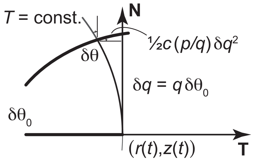
Fig. 4: Phase of the Gaussian beam along the ray’s extrinsic normal ${\mathbf{N}}=d{\mathbf{T}}/ds$. The differential time $\delta t_{\rm e}$ a distance $\delta\eta$ along the normal is given by the quadratic $\delta t_{\rm e}={\textstyle{1\over 2}}(p/q)\,\delta\eta^{2}={\textstyle{1\over 2}}c^{-2}({\kern 1.00006pt\raise 1.29167pt\hbox{$\dot{\ayn}$}\kern 0.50003pt}/{\kern 1.00006pt\raise 1.29167pt\hbox{$\ayn$}\kern 0.50003pt}+c^{\prime}\sin\theta)\,\delta\eta^{2}$. All distances in the figure represent extrinsic Euclidean distances.

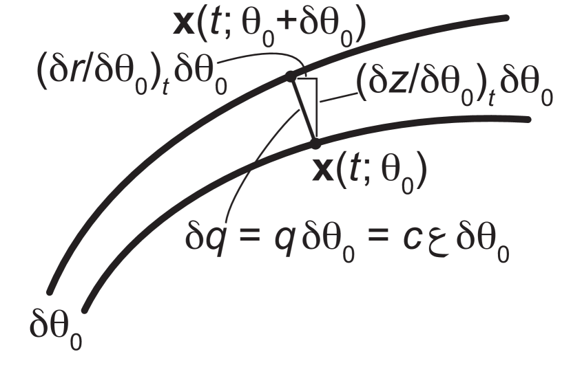
Fig. 5: Geometric spreading expressed using ray-centered and extrinsic range and depth coordinates. All distances in the figure represent extrinsic Euclidean distances.

3.3 Transverse Phase of a Gaussian Beam

The differential time $\delta t_{\rm e}$ perpendicular to the ray (extrinsic) determines the differential phase $e^{j\,\delta\varphi}$ of the Gaussian beam, where ${\delta\varphi=2\pi f_{c}\,\delta t_{\rm e}}$, $f_{c}$ is the center or carrier frequency of the sound propagating along the ray, and ${j=\sqrt{-1}}$. In terms of the extrinsic geometric spreading variables $q$ and ${p=\partial T/\partial q}$, the differential time a distance $\delta\eta$ along the ray normal at ${\bigl{(}r(s),z(s)\bigr{)}^{\scriptscriptstyle\rm T}}$ is given by the formulae [16, 22]

$$\delta t_{\rm e}={1\over 2}{p\over q}\,\delta\eta^{2}={1\over 2}\left({{\kern 1.00006pt\raise 1.29167pt\hbox{$\dot{\ayn}$}\kern 0.50003pt}\over{\kern 1.00006pt\raise 1.29167pt\hbox{$\ayn$}\kern 0.50003pt}}+c^{\prime}\sin\theta\right)\,\delta\mu^{2},$$ (31)

where ${\delta\mu=c^{-1}\,\delta\eta}$. This fact is illustrated in Fig. 4. To compare this extrinsic formula with the intrinsic results developed in section 3.7, it is worthwhile to give a brief geometric proof of Eq. (31). By inspection, or formally by Gauss’s lemma of Eq. (28) the differential path time along the ray normal is a quadratic function of distance up to second order, i.e.

$$\delta t_{\rm e}={\textstyle{1\over 2}}Q_{\rm e}\,\delta\eta^{2}$$ (32)

for some quadratic coefficient $Q_{\rm e}$ to be determined. As seen in Fig. 4, the slope of this quadratic function at $\delta\eta$ equals $\delta\theta$, the differential change in angle:

$$\delta\theta=cd(\delta t_{\rm e})/d(\delta\eta)|_{\delta\eta=\delta q=q\,\delta\theta_{0}}=cQ_{\rm e}\,\delta q=cqQ_{\rm e}\,\delta\theta_{0}.$$ (33)

However, $\delta\theta$ may be computed directly via an inner product along with Eq. (LABEL:eq:qde),

$$\delta\theta=\langle{\mathbf{N}},(d/ds){\mathbf{x}}(s;\theta_{0}+\delta\theta_{0})\rangle=\bigl{\langle}{\mathbf{N}},(d/ds)\bigl{(}{\mathbf{x}}(s;\theta_{0})+q\,\delta\theta_{0}\,{\mathbf{N}}\bigr{)}\bigr{\rangle}=cp\,\delta\theta_{0}$$ (34)

Equating $\delta\theta$ from Eqs. (33) and (34) yields ${Q_{\rm e}=p/q}$, from which Eq. (32) becomes the first equality of Eq. (31). Applying Eq. (LABEL:eq:tildeqde) to Eq. (31) yields

$$c^{2}{p\over q}={{\kern 1.00006pt\raise 1.29167pt\hbox{$\dot{\ayn}$}\kern 0.50003pt}\over{\kern 1.00006pt\raise 1.29167pt\hbox{$\ayn$}\kern 0.50003pt}}+c^{\prime}\sin\theta$$ (35)

and the second equality.

Summarizing the results of the previous sections, the transverse amplitude and phase of a Gaussian beam emanating a distance $\delta\eta$ normal to the ray and with initial source level SL and azimuth end elevation angle fan widths $\delta\phi_{0}$ and $\delta\theta_{0}$ is given by

$$P(s;\theta_{0};\delta\mu) = \left[{\hbox{SL}{\cdot}c_{s}\cos\theta_{0}\over c_{0}rq}\right]^{{1\over 2}}\exp\left[j2\pi f_{c}\left(t(s)+{p\over 2q}\,\delta\eta^{2}\right)\right]$$ (37)

$$\left[{\hbox{SL}{\cdot}a\over r{\kern 1.00006pt\raise 1.29167pt\hbox{$\ayn$}\kern 0.50003pt}}\right]^{{1\over 2}}\exp\left[j2\pi f_{c}\left(t+{1\over 2}\left({{\kern 1.00006pt\raise 1.29167pt\hbox{$\dot{\ayn}$}\kern 0.50003pt}\over{\kern 1.00006pt\raise 1.29167pt\hbox{$\ayn$}\kern 0.50003pt}}+c^{\prime}\sin\theta\right)\,\delta\mu^{2}\right)\right].$$

Note that Gaussian beam is an appropriate name for rays with this functional form. A Gaussian distribution of amplitude is typically introduced through the initial conditions for the Gaussian beam.

3.4 Munk, Linear, and SSPs with Constant Curvature

3.4.1 Munk Profile

The distance between convergence zones/cycle distances for the Munk profile $c(z)=c_{0}\bigl{(}1+\epsilon(\bar{z}+e^{-\bar{z}}-1)\bigr{)}$ with ${\bar{z}=(z-z_{0})/W}$ can be computed directly via Eq. (25). At ${z=z_{0}}$, the Gaussian curvature $K=cc^{\prime\prime}-(c^{\prime})^{2}=\epsilon c_{0}^{2}/W^{2}$, proving the new theorem:

Theorem 6.

The cycle distance of the Munk profile approximately equals

$${\hbox{Munk profile}\atop\hbox{CZ distance}}\approx\pi\epsilon^{-1/2}W.$$ (38)

E.g. for the nominal parameters ${\epsilon=0.00737}$ and ${W=650\,}$m, this yields a distance of $23.8\,$km (Fig. 1).

3.4.2 Linear SSPs

The ideas developed to this point are nicely illustrated using the example of Gaussian beams in medium with linear SSP ${c(z)=c_{0}+\gamma z}$, in which case rays are simply circles in $(r,z)$-space: [22]

$$r(\theta) = z_{0\gamma}\sec\theta_{0}\bigl{(}\sin\theta_{0}+\sin(\theta-\theta_{0})\bigr{)},$$ (39)

$$z(\theta) = -c_{0}\gamma^{-1}+z_{0\gamma}\sec\theta_{0}\cos(\theta-\theta_{0}),$$ (40)

where the ray emanates from $(0,z_{0})$ with initial elevation angle $\theta_{0}$, and ${z_{0\gamma}=z_{0}+c_{0}\gamma^{-1}}$. Arclength is given by ${s=z_{0\gamma}\theta}$, and eigenrays to $(r,z)$ are determined by the angles

$$\theta_{0} = 2\operatorname{atan2}\Bigl{(}2rz_{0\gamma}-\bigl{(}r^{2}+(z_{0\gamma}-z)^{2}\bigr{)}\bigl{(}r^{2}+(z_{0\gamma}+z)^{2}\bigr{)},z_{0\gamma}^{2}-z^{2}-r^{2}\Bigr{)}^{1\over 2},$$ (41)

$$\theta = \operatorname{atan2}(r-z_{0\gamma}\tan\theta_{0},z+c_{0}\gamma^{-1})+\theta_{0},$$ (42)

with travel-time

$$t={1\over\gamma}\log\left({\tan{\textstyle{1\over 2}}\sin^{-1}\cos\theta_{0}\over\tan{\textstyle{1\over 2}}\sin^{-1}\left({c_{0}+\gamma z\over c_{0}+\gamma z_{0}}\cos\theta_{0}\right)}\right),$$ (43)

assuming no caustics along the ray. Because ${c_{\rm nn}\equiv 0}$, the Hamilton equations (LABEL:eq:qde)–(LABEL:eq:pde) are easily solved in closed form,

$$q=z_{0\gamma}\sec^{2}\theta_{0}\Bigl{(}\bigl{(}1-a^{2}(c_{0}+\gamma z)^{2}\bigr{)}^{1/2}-|\sin\theta_{0}|\Bigr{)},\quad\hbox{and}\quad p={1\over c_{0}+\gamma z_{0}}.$$ (44)

Likewise, because the Gaussian curvature ${K\equiv-\gamma^{2}}$ is constant (the propagation medium is a space of constant negative curvature, i.e. it is a hyperbolic space), Jacobi’s equation (20) has the closed-form solution ${\kern 1.00006pt\raise 1.29167pt\hbox{$\ayn$}\kern 0.50003pt}(t)=\gamma^{-1}\sinh\gamma t$, or ${{\kern 1.00006pt\raise 1.29167pt\hbox{$\ayn$}\kern 0.50003pt}(t)\approx t+{1\over 6}\gamma^{2}t^{3}}$ for ${t\lessapprox\gamma^{-1}}$, yielding $q=c\gamma^{-1}\sinh\gamma t\approx{ct(1+{1\over 6}\gamma^{2}t^{2})}$, a much simpler expression than Eq. (44). The expression for the relative delay is given by ${p/q\approx c_{1}^{-1}c^{-1}t^{-1}(1-{1\over 6}\gamma^{2}t^{2})}$, a new result.

3.4.3 SSPs with Constant Curvature

The linear SSP example above is an example of a medium with constant (negative) Gaussian curvature—a hyperbolic space. In general, it is worthwhile to ask which SSPs yield spaces of constant positive or negative curvature, because these SSPs serve as models for both convergent and divergent ray propagation. Solving the 2d order nonlinear differential equation ${cc^{\prime\prime}-(c^{\prime})^{2}=K}$ for constant $K$ yields,

$$\halign to=433.62pt{\hfil\hskip\@centering$\displaystyle{#}$\@eqnsel&\global\@eqcnt\@ne\hskip\tw@\eqncolsep\hfil${{}#{}}$\hfil&\global\@eqcnt\tw@\hskip 1\eqncolsep$\displaystyle{#}$\hfil&\qquad\hskip\@centering\hfil$\displaystyle{#}$\@eqnsel&\global\@eqcnt\@ne\hskip\tw@\eqncolsep\hfil${{}#{}}$\hfil&\global\@eqcnt\tw@\hskip\tw@\eqncolsep$\displaystyle{#}$\hfil&\global\@eqcnt\thr@@\hb@xt@\z@\bgroup\hss#\egroup\cr 0.0pt plus 1000.0pt$\displaystyle{c(z)&0.0pt\hfil${{}=&0.0pt$\displaystyle{c_{0}\cosh(z-z_{0})/W;&0.0pt plus 1000.0pt\hfil$\displaystyle{K&0.0pt\hfil${{}=&0.0pt$\displaystyle{c_{0}^{2}/W^{2}>0,\\ c(z)&\hbox to0.0pt{\hss=}&c_{0}\sinh(z-z_{0})/W;&K&=&-c_{0}^{2}/W^{2}<0,\\c(z)&=&c_{0}\cos(z-z_{0})/W;&K&=&-c_{0}^{2}/W^{2}<0,\\c(z)&=&c_{0}\sin(z-z_{0})/W;&K&=&-c_{0}^{2}/W^{2}<0,\\c(z)&=&c_{0}+\gamma z;&K&=&-\gamma^{2}\leq 0,\cr}}}}}}}$$

of which only the first has constant positive curvature.

The hyperbolic cosine SSP $c(z)=c_{0}\cosh({z-z_{0}})/W\approx c_{0}+{\textstyle{1\over 2}}c_{0}W^{-2}({z-z_{0}})^{2}$ is the solution for an acoustic duct, which traps rays near depth $z_{0}$. Regions modeled by hyperbolic cosine SSPs are described in the literature with increasing frequency, [35, 14, 36, 40, 28, 25, 8, 37, 21]; Bergman [8] observes that this profile yields constant curvature. The solution to Jacobi’s equation for intrinsic geometric spreading in Theorem 5 equals ${{\kern 1.00006pt\raise 1.29167pt\hbox{$\ayn$}\kern 0.50003pt}(t)=K^{-{1\over 2}}\sin K^{1\over 2}t}$, with half-wavelength travel-time between caustics determined by ${\pi K^{-{1\over 2}}=\pi W/c_{0}}$ [cf. Eq. (25)]. The range between caustics equals $c_{0}$ times the travel-time for all small initial elevation angles $\theta_{0}$; therefore, by invariance, the range between caustics for all initial elevation angles necessarily equals $\pi W$, yielding the following new and useful theorem [35, 14, 36, 8]:

Theorem 7.

Let ${c(z)=c_{0}\cosh(z-z_{0})/W}$ be a SSP with hyperbolic cosine profile. Then for any initial elevation angle $\theta_{0}$, speed $c_{0}$, and depth $z_{0}$, the range between caustics and focusing regions is given by the constant,

$${\hbox{half-wavelength}\atop\hbox{range}}=\pi c_{0}K^{-1/2}=\pi W.$$ (46)

This theorem is illustrated in Fig. 2 over a large range of initial elevation angles. Porter [28] uses a value of ${W^{-1}=0.0003}\,\hbox{m}^{-1}$ for his hyperbolic cosine SSP and observes without explanation that “the rays refocus perfectly at distances of about every $10\,$km.” Indeed, Theorem 7 establishes that all rays refocus perfectly every ${\pi/0.0003=10.47}\,$km, precisely as shown in Porter’s Fig. 8 on p. 2020. [28] This is also verified by the closed-form functional form of rays with SSP, available from Snell’s law, $\cosh({z-z_{0}})/W=\sec\theta_{0}\*\bigl{(}{1-\sin^{2}\theta_{0}\cos^{2}(r/W)}\bigr{)}^{1\over 2}$; the property of constant curvature also yields a simple solutions for the intrinsic geometric spreading ${{\kern 1.00006pt\raise 1.29167pt\hbox{$\ayn$}\kern 0.50003pt}(t)=(c_{0}/W)\sin(c_{0}t/W)}$ and both the intrinsic phase ${{\kern 1.00006pt\raise 1.29167pt\hbox{$\dot{\ayn}$}\kern 0.50003pt}/{\kern 1.00006pt\raise 1.29167pt\hbox{$\ayn$}\kern 0.50003pt}=(W/c_{0})\cot(c_{0}t/W)}$ and extrinsic phase $p/q$ via Eq. (35). In practice, it is the quadratic term ${\cosh z\approx 1+{\textstyle{1\over 2}}z^{2}}$ of the hyperbolic cosine profile that dominates ray behavior in a duct, and ducting regions with quadratic SSPs and approximately constant positive curvature are quite common. This establishes the approximate distance between caustics in a duct given in Eq. (25).

In all other solutions with physical positive speed ${c(z)>0}$, the Gaussian curvature is a negative constant, and rays diverge from each other according to the intrinsic geometric spreading ${{\kern 1.00006pt\raise 1.29167pt\hbox{$\ayn$}\kern 0.50003pt}(t)=K^{-{1\over 2}}\sinh K^{{1\over 2}}t}\approx{t+{1\over 6}Kt^{3}}$, which equals ${t+{1\over 6}(c_{0}^{2}/W^{2}){\cdot}t^{3}}$ for the downward refracting SSP ${c(z)=c_{0}\sinh(z-z_{0})/W}$ and the trigonometric SSPs ${c(z)=c_{0}\cos(z-z_{0})/W}$ with divergence zones. The trigonometric SSPs of constant negative curvature with convergent ducts (such that ${c^{\prime\prime}>0}$) are in fact nonphysical because the sound speed must be negative at such depths; physical ducting behavior with positive sound speed is described by the first hyperbolic cosine solution. The case of linear SSPs, whose constant curvature is negative, is treated in the previous subsection. Finally, SSPs with vanishing constant curvature ${K\equiv 0}$ and intrinsic geometric spreading ${{\kern 1.00006pt\raise 1.29167pt\hbox{$\ayn$}\kern 0.50003pt}(t)=t}$ are obviously given by the SSP with constant speed $c_{0}$.

3.5 Beam Amplitude and Phase Based Upon Snell’s Law

From Fig. 5 it is graphically obvious that the geometric spreading $q(t)=\|(\partial{\mathbf{x}}(t;\theta_{0})/\partial\theta_{0})_{t}\|_{2}$ satisfies the trigonometric relationships

$$q=c{\kern 1.00006pt\raise 1.29167pt\hbox{$\ayn$}\kern 0.50003pt}=\left(\left({\partial r\over\partial\theta_{0}}\right)_{t}^{2}+\left({\partial z\over\partial\theta_{0}}\right)_{t}^{2}\right)^{1/2}\\=\left({\partial r\over\partial\theta_{0}}\right)_{z}\sin\theta=-\left({\partial z\over\partial\theta_{0}}\right)_{r}\cos\theta,$$ (47)

where $\theta={\tan^{-1}(\dot{z}/\dot{r})}$ is the elevation angle of the ray at point $t$. This figure is drawn using an implicit assumption Gauss’s lemma, namely that the tangent vectors $\dot{\mathbf{x}}$ and $(\partial{\mathbf{x}}/\partial\theta_{0})_{t}$ are perpendicular. It is therefore instructive in establishing the relationship between Snell’s law and the intrinsic approach to show how Gauss’s law imply Eqs. (47). An additional benefit will be an equation for the transverse phase of a Gaussian beam expressed in Snell’s law form.

The first-order Taylor series expansion of the expressions $r(t;\theta_{0})$ and $z(t;\theta_{0})$ yield

$$\delta r=\dot{r}\,\delta t_{\rm e}+(\partial r/\partial\theta_{0})_{t}\,\delta\theta_{0},\quad\hbox{and}\quad\delta z=\dot{z}\,\delta t+(\partial z/\partial\theta_{0})_{t}\,\delta\theta_{0}.$$ (48)

Fixing the variables $z$ and $r$, i.e. ${\delta z=0}$ and ${\delta r=0}$ respectively, yields the relationships

$$(\partial r/\partial\theta_{0})_{z}=-\cot\theta\cdot(\partial z/\partial\theta_{0})_{r}=(\partial r/\partial\theta_{0})_{t}-\cot\theta\cdot(\partial z/\partial\theta_{0})_{t}$$ (49)

between partial derivatives. Gauss’s lemma [Eq. (28)] provides the additional relationship

$$(\partial r/\partial\theta_{0})_{t}+\tan\theta\cdot(\partial z/\partial\theta_{0})_{t}=0$$ (50)

that along with Eq. (49) yields Eq. (47). The conclusion is that the intrinsic geometric spreading

$${\kern 1.00006pt\raise 1.29167pt\hbox{$\ayn$}\kern 0.50003pt}=c^{-1}(\partial r/\partial\theta_{0})_{z}\sin\theta=-c^{-1}(\partial z/\partial\theta_{0})_{r}\cos\theta$$ (51)

in Snell’s law form satisfies Jacobi’s equation [Eq. (20)], where $r(z;\theta_{0})$ is given by Snell’s law [Eq. (3)].

A benefit of this intrinsic viewpoint of Snell’s law is a new expression for the transverse phase of a Gaussian beam, obtained by direct application of Eq. (35) to Eqs. (3) and (47). Differentiating the first equality of Eq. (47) w.r.t. $s$ and applying the identities ${dz/ds=\sin\theta}$ the Frenet-Serret equations of section 2.1 yields

$$p/q={1\over c}\left({\partial r\over\partial\theta_{0}}\right)_{z}^{-1}\left({\partial r\over\partial\theta_{0}}\right)_{z}^{\prime}\sin\theta+{c^{\prime}\over c^{2}}{\cos^{2}\theta\over\sin\theta},$$ (52)

where $({\partial r/\partial\theta_{0}})_{z}^{\prime}=(d/dz)({\partial r/\partial\theta_{0}})_{z}$ as usual. These terms are immediately available via Eq. (3):

$$\left({\partial r\over\partial\theta_{0}}\right)_{z} = -{\sin\theta_{0}\over c(z_{0})}\int_{z_{0}}^{z}{c(z_{\prime})\over\bigl{(}1-a^{2}c^{2}(z_{\prime})\bigr{)}^{3/2}}\,dz_{\prime},$$ (53)

$$\left({\partial r\over\partial\theta_{0}}\right)_{z}^{\prime} = -{\sin\theta_{0}\over c(z_{0})}{c(z)\over\bigl{(}1-a^{2}c^{2}(z)\bigr{)}^{3/2}}.$$ (54)

Likewise, differentiating the first equality of Eq. (51) w.r.t. $t$ yields ${{\kern 1.00006pt\raise 1.29167pt\hbox{$\dot{\ayn}$}\kern 0.50003pt}/{\kern 1.00006pt\raise 1.29167pt\hbox{$\ayn$}\kern 0.50003pt}=c^{2}p/q-c^{\prime}\sin\theta}$, consistent with Eqs. (19) and (35).

3.6 Beam Amplitude and Phase Based Upon Ray Angle

The derivation of the phase of a Gaussian beam above leads to another formulation of the amplitude of a Gaussian beam, which has been used in Gaussian beam applications. Eqs. (LABEL:eq:qde) and (34) implies that up to second order in $\delta\theta_{0}$,

$$q(s)=\int_{0}^{s}(\partial\theta/\partial\theta_{0})_{s_{\prime}}\,ds_{\prime},$$ (55)

a formula that has been used by others to compute the extrinsic geometric spreading. The transverse phase of a Gaussian beam, up to second-order, is then given by

$${cp\over q}=\left(\int_{0}^{s}\left({\partial\theta\over\partial\theta_{0}}\right)_{s_{\prime}}\,ds_{\prime}\right)^{-1}\left({\partial\theta\over\partial\theta_{0}}\right)_{s}$$ (56)

and Eq. (31).

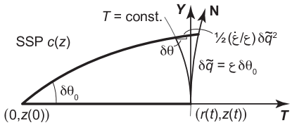
Fig. 6: Intrinsic view of ray tube in a horizontally stratified medium, in the tangent plane at the point $\bigl{(}0,z(0)\bigr{)}$. The azimuthal component, not shown, is perpendicular to the page. All distances in the figure represent travel-time, not Euclidean distance. Note that the extrinsic ray normal ${{\mathbf{N}}=d{\mathbf{T}}/ds}$—the straight line in extrinsic coordinates used to define $\delta q$ in Eq. (4)—is not straight using intrinsic coordinates and diverges a small amount from the time-minimizing geodesic in the normal direction, shown here as the vector ${\bm{Y}}$. The extrinsic normal vector ${\mathbf{N}}$ is preferred for numerical computation of the differential path time ${\delta t_{\rm e}={\textstyle{1\over 2}}(p/q)\,\delta\eta^{2}}$; however, the intrinsic normal vector ${\bm{Y}}$, from which the differential travel-time is given by $\delta t_{\rm i}={\textstyle{1\over 2}}(c^{-2}{\kern 1.00006pt\raise 1.29167pt\hbox{$\dot{\ayn}$}\kern 0.50003pt}/{\kern 1.00006pt\raise 1.29167pt\hbox{$\ayn$}\kern 0.50003pt})\,\delta\eta^{2}={\textstyle{1\over 2}}(p/q-c^{\prime}\sin\theta),\delta\eta^{2}$, appears in the intrinsic formulation of Gaussian beam. The path time along either intrinsic ${\bm{Y}}$ or extrinsic ${\mathbf{N}}$ equals ${\delta\tilde{q}={\kern 1.00006pt\raise 1.29167pt\hbox{$\ayn$}\kern 0.50003pt}\,\delta\theta_{0}}$ to first-order.

3.7 Intrinsic Transverse Amplitude and Phase of a Gaussian beam

The amplitude and phase of a Gaussian beam has been fully developed in section 3 for the computationally practical case of a Gaussian beam defined extrinsically along a straight line normal to the ray. In this section, it is explained how Jacobi’s equation quantifies precisely the same construct intrinsically, if the extrinsic straight line in ${(r,z)}$-space is replaced with an intrinsic geodesic normal to the ray. Fig. 6 illustrates the difference: because “straight lines” in ${(r,z)}$-space are actually curved intrinsically—they are not time minimizing geodesics—there is a small difference between the differential path times. This accounts for the extra term $c^{\prime}\sin\theta$ seen in Eqs. (19), (35), and (37). Though computationally impractical, the following new theorem connects Jacobi’s equation with the differential path time along rays normal to the ray at the center of the Gaussian beam.

Theorem 8.

(Intrinsic transverse phase of a Gaussian beam, $2$-d case)  Let $\delta t_{\rm i}$ be the travel-time difference between the surface of constant travel-time $t$ and an intrinsic distance $\delta\mu$ along the intrinsic transverse plane (i.e. defined by geodesics) to the ray at point ${\mathbf{x}}(t;\theta_{0})$, and let ${\kern 1.00006pt\raise 1.29167pt\hbox{$\ayn$}\kern 0.50003pt}(t)$ be the solution to Jacobi’s equation [Eq. (20)] along the ray. Then

$$\delta t_{\rm i}={1\over 2}{{\kern 1.00006pt\raise 1.29167pt\hbox{$\dot{\ayn}$}\kern 0.50003pt}\over{\kern 1.00006pt\raise 1.29167pt\hbox{$\ayn$}\kern 0.50003pt}}\,\delta\mu^{2}+O(\delta\mu^{3}).$$ (57)

The proof of Theorem 8 involves another application of Gauss’s lemma and a Taylor series expansion about ${\mathbf{x}}(t;\theta_{0})$, and is comparable to the proof of Eq. (31) above. Consider the change of elevation angle $\theta(t)={\tan^{-1}(\dot{z}/\dot{r})}$ of the ray: let $\delta\theta$ be the difference between $\theta$ and the slope of the ray ${\mathbf{x}}(t;{\theta_{0}+\delta\theta})$ intersecting the transverse plane at distance $\delta\mu={\kern 1.00006pt\raise 1.29167pt\hbox{$\ayn$}\kern 0.50003pt}\,\delta\theta_{0}$ along a geodesic emanating perpendicularly from the ray with initial unit tangent vector ${\bm{Y}}$, i.e. ${g({\bm{Y}},{\bm{Y}})=1}$ and ${g({\bm{T}},{\bm{Y}})=0}$. This definition of $\delta\theta$ equates to the relation

$$\delta\theta=\langle{\bm{Y}},\tau_{\delta\mu}^{-1}\dot{\mathbf{x}}(t;\theta_{0}+\delta\theta)-\dot{\mathbf{x}}(t;\theta_{0})\rangle,$$ (58)

where $\tau_{\delta\mu}^{-1}$ is the inverse parallel translation along the geodesic between the points ${\mathbf{x}}(t;\theta_{0})$ and ${\mathbf{x}}(t;{\theta_{0}+\delta\theta})$ in direction ${\bm{Y}}$. A straightforward Taylor series analysis of the differential equations describing parallelism [20] shows that for any arbitrary vector field ${\bm{X}}(\delta\mu)$, $\tau_{\delta\mu}^{-1}{\bm{X}}(\delta\mu)={\bm{X}}(0)+O(\delta\mu^{2})$—the proof involves so-called “normal coordinates” defined so that at the single point where $\delta\mu=0$, $g_{ij}(0)=\delta_{ij}$ and rays in the direction ${\bm{Y}}$ have the coordinates $(tY^{1},tY^{2})$, implying that $\Gamma^{k}_{ij}(0)=0$. The implication of this local analysis about the point ${\mathbf{x}}(t;\theta_{0})$ is that

$$\delta\theta={\kern 1.00006pt\raise 1.29167pt\hbox{$\dot{\ayn}$}\kern 0.50003pt}\,\delta\theta_{0}+O(\delta\theta_{0}^{2})$$ (59)

because, up to second order,

$$\dot{\mathbf{x}}(t;{\theta_{0}+\delta\theta})=(d/dt)\bigl{(}{\mathbf{x}}(t;{\theta_{0}})+{\kern 1.00006pt\raise 1.29167pt\hbox{$\ayn$}\kern 0.50003pt}(t){\bm{Y}}(t)\bigr{)}=\dot{\mathbf{x}}(t;\theta_{0})+{\kern 1.00006pt\raise 1.29167pt\hbox{$\dot{\ayn}$}\kern 0.50003pt}{\bm{Y}}+{\kern 1.00006pt\raise 1.29167pt\hbox{$\ayn$}\kern 0.50003pt}\nabla_{\bm{T}}{\bm{Y}}=\dot{\mathbf{x}}(t;\theta_{0})+{\kern 1.00006pt\raise 1.29167pt\hbox{$\dot{\ayn}$}\kern 0.50003pt}{\bm{Y}}$$ (60)

by the parallelism of ${\bm{Y}}$ along the ray. Now the change in slope $\delta t_{\rm i}$ of the ray is equal to the slope of the quadratic function $\delta t_{\rm i}={(1/2)Q_{\rm i}\,\delta\mu^{2}+O(\delta\mu^{3})}$ for some coefficient $Q_{\rm i}$ that is implied by Gauss’s lemma. The slope of this function at $\delta\mu$ equals

$$\delta\theta+O(\delta\theta^{3})=\tan\delta\theta=d(\delta t_{\rm i})/d(\delta\mu)=Q_{\rm i}\,\delta\mu=Q_{\rm i}{\kern 1.00006pt\raise 1.29167pt\hbox{$\ayn$}\kern 0.50003pt}\,\delta\theta_{0}.$$ (61)

Equating Eqs. (59) and (61), we conclude that ${Q_{\rm i}={\kern 1.00006pt\raise 1.29167pt\hbox{$\dot{\ayn}$}\kern 0.50003pt}/{\kern 1.00006pt\raise 1.29167pt\hbox{$\ayn$}\kern 0.50003pt}}$, establishing the theorem.

The quadratic coefficient ${\kern 1.00006pt\raise 1.29167pt\hbox{$\dot{\ayn}$}\kern 0.50003pt}/{\kern 1.00006pt\raise 1.29167pt\hbox{$\ayn$}\kern 0.50003pt}$ for the phase is physically consistent with two easily imagined examples. For flat space where the Gaussian curvature vanishes, ${\kern 1.00006pt\raise 1.29167pt\hbox{$\ayn$}\kern 0.50003pt}(t)\equiv t$, ${\kern 1.00006pt\raise 1.29167pt\hbox{$\dot{\ayn}$}\kern 0.50003pt}(t)\equiv 1$, and the wavefront of constant $t$ is a circle of radius $t$, in which case the gap size equals $\delta t_{\rm i}-{t\sec\delta\theta_{0}-t}={(t/2)(\delta\theta_{0})^{2}+O(h^{4})}={(1/2)(1/t)(\delta\mu)^{2}+O(h^{4})}$, as predicted by Theorem 8. For the second example, consider acoustic propagation in a space of constant positive curvature $K=R^{-2}$, e.g. S-waves emanating from a (geologically unlikely) earthquake on the north pole of the earth. In this case the rays are all great circles on the sphere that intersect at the north pole, i.e. longitudinal lines. At every point around the equator, equivalently, in the plane transverse to every ray at the equator, all rays have equal travel-time to the north pole; therefore, $\delta t_{\rm i}=0$ around the equator. Indeed, solving Jacobi’s equation [Eq. (20)] yields ${\kern 1.00006pt\raise 1.29167pt\hbox{$\ayn$}\kern 0.50003pt}(t)=\sin(t/R)$ for which ${\kern 1.00006pt\raise 1.29167pt\hbox{$\dot{\ayn}$}\kern 0.50003pt}={\cos({1\over 2}\pi)=0}$ at the equator, an easily obtained intuitive result that is again consistent with Theorem 8.

4 Conclusions

Paraxial ray theory is an essential and useful component of modern acoustic modeling. There are deep and important connections between the classically derived paraxial ray equations for the amplitude and phase along a Gaussian beam, and the second-order variation—called Jacobi’s equation—along geodesics encountered in differential geometry. This paper demonstrates how known results in paraxial ray theory correspond to their counterparts in differential geometry, and shows how both new equations and new insights into the properties of acoustic rays are obtained from an intrinsic, differential geometric point of view. It is shown how the intrinsic Gaussian curvature affect the spreading of Gaussian beams, and how the specific form of this intrinsic curvature [${K=cc^{\prime\prime}-(c^{\prime})^{2}}$ for a horizontally stratified medium with SSP $c(z)$] allows one to easily compute the distance between caustics within a duct, as well as the geometric spreading for either a duct or a region with linear SSP. These results allow the introduction of SSPs yielding constant Gaussian curvature, which serve as model spaces for both convergent acoustic ducts (positive curvature), divergence zones (negative curvature), and non-refractive spreading (zero curvature). It is proved for the model of a hyperbolic cosine SSP, the range between caustics is constant for all rays. Intrinsic versions of the amplitude and Gaussian beams are introduced. The intrinsic geometric spreading is shown to be equivalent to its extrinsic counterpart after scaling by the position-dependent sound speed. The intrinsic phase of a Gaussian beam, which is the phase along geodesics, not straight lines, emanating in a normal direction from the ray, is shown to be equivalent up to a small additive term to the phase of a paraxial ray as it is typically defined. Because the differential geometric approach is quite general, all results may be generalized to three dimensions, and in all cases, the connection is made with known results derived from either Snell’s law, Hamilton’s equations, or the Frenet-Serret formulae. The results may also be applied to other special cases of applied interest, such as a spherically stratified sound speed.

References

- [1]
- [2]
- [3]
- [4]
- [5]
- [6] D. R. Bergman, Application of differential geometry to acoustics: Development of a generalized paraxial ray-trace procedure from geodesic deviation, Technical Report NRL/MR/7140–05-8835, Naval Research Laboratory, 2005.
- [7] , Generalized space-time paraxial acoustic ray tracing, Waves in Random and Complex Media, 15 (2005), pp. 417–435.
- [8] , Internal symmetry in acoustical ray theory, Wave Motion, 43 (2006), pp. 508–516.
- [9] L. Bos and M. A. Slawinski, Regions of invalidity of ray-centered coordinates, Q. J. Mech. Appl. Math., 63 (2) (2010), pp. 227–236.
- [10] L. Bos and M. A. Slawinski, Elastodynamic equations: Characteristics, wavefronts, and rays, Q. J. Mech. Appl. Math., 63 (1) (2009), pp. 23–37.
- [11] L. M. Brekhovskikh, Waves in Layered Media, 2d edition, Academic Press, New York, 1980, p. 374.
- [12] L. M. Brekhovskikh and O. A. Godin, Acoustics of Layered Media II, 2d edition, Springer-Verlag, Berlin, 1999, pp. 85–86.
- [13] L. M. Brekhovskikh and Yu. P. Lysanov, Fundamentals of Ocean Acoustics, 3d edition, American Institute of Physics Press, New York, 2003, p. 141.
- [14] H. K. Brock, R. N. Buchal, and C. W. Spofford, Modifying the sound speed profile to improve the accuracy of the parabolic equation technique, J. Acoust. Soc. Am., 62 (1977), pp. 543–552.
- [15] V. Červený, Ray tracing algorithms in three-dimensional laterally varying layered structures, in Seismic Tomography, D. Reidel Publishing Co., Dordrecht, Holland, 1987, pp. 99–133.
- [16] , Seismic Ray Theory, chapter 4, Cambridge University Press, 2001, pp. 237–267.
- [17] J. Cheeger and D. G. Ebin, Comparison Theorems in Riemannian Geometry, chapter 1, North-Holland Publishing Company, Amsterdam, 1975.
- [18] C. S. Clay and H. Medwin, Acoustical Oceanography: Principles and Applications, chapter 3, Wiley, New York, 1977.
- [19] I. M. Gelfand and S. V. Fomin, Calculus of Variations, chapter 5, Prentice-Hall, Inc., Englewood Cliffs, NJ, 1963.
- [20] S. Helgason, Differential Geometry, Lie Groups, and Symmetric Spaces, chapter , Academic Press, New York, 1978.
- [21] U. Ingard, Noise Reduction Analysis, Jones & Bartlett, Sudbury MA, 2010, p. 354.
- [22] F. B. Jensen, W. A. Kuperman, M. B. Porter, and H. Schmidt, Computational Ocean Acoustics, 2d. ed., chapter 3, American Institute of Physics Press, New York, 2011.
- [23] N. Jobert, G. Jobert, and G. Nolet, Ray tracing for surface waves, in Seismic Tomography, D. Reidel Publishing Co., Dordrecht, Holland, 1987, pp. 275–300.
- [24] H. B. Keller and D. J. Perozzi, Fast seismic ray tracing, SIAM J. Appl. Math., 43 (1983), pp. 981–992.
- [25] M. M. Kordich and D. A. Pollet, Sound intensity prediction system (SIPS): Volume 1—Reference manual, Technical Report NSWCDD/TR-97/144, Naval Surface Warfare Center, Dahlgren Division, Dahlgren, VA, 1997.
- [26] B. Nair and B. S. White, High-Frequency wave propagation in random media—a unified approach, SIAM J. Appl. Math., 51 (1991), pp. 374–411.
- [27] A. D. Pierce, Acoustics, Acoustical Society of America, New York, 1989, pp. 371–419.
- [28] M. B. Porter, The time-marched fast-field program (FFP) for modeling acoustic pulse propagation, J. Acoust. Soc. Am., 87 (1990), pp. 2013–2023.
- [29] M. B. Porter and H. P. Bucker, Gaussian beam tracing for computing ocean acoustic fields, J. Acoust. Soc. Am., 89 (1987), pp. 1349–1359.
- [30] R. Rashed, A pioneer in anaclastics: Ibn Sahl on burning mirrors and lenses, Isis, 81 (1990), pp. 464–491.
- [31] J. W. S. Rayleigh, Theory of Sound, volume 2, reprint of the 1895 edition, Dover, New York, 1945, p. 129
- [32] H. Rund, The Differential Geometry of Finsler Spaces, Springer-Verlag, Berlin, 1959.
- [33] M. C. Shen and J. B. Keller, Uniform ray theory of surface, internal and acoustic wave propagation in a rotating ocean or atmosphere, SIAM J. Appl. Math., 28 (1975), pp. 857–875.
- [34] M. Spivak, A Comprehensive Introduction to Differential Geometry, vols. 2, 4, chapter 4, 3d edition, Publish or Perish, Inc., Houston, TX, 1999.
- [35] I. Tolstoy and C. S. Clay, Ocean Acoustics Theory and Experiment in Underwater Sound, McGraw-Hill, Inc., New York, 1966, p. 156.
- [36] A. Tolstoy, D. H. Berman, and E. R.Franchi Ray theory versus the parabolic equation in a long-range ducted environment, J. Acoust. Soc. Am., 78 (1985), pp. 176–189.
- [37] R. A. Vadov, Regional distinctions in the time structure of the sound field produced by a point source in the underwater sound channel, J. Acoustical Physics, 52 (2006), pp. 533–543.
- [38] E. K. Westwood and P. J. Vidmar, Eigenray finding and time series simulation in a layered-bottom ocean, J. Acoust. Soc. Am., 81 (1987), pp. 912–924.
- [39] K. B. Wolf and G. Krötzsch, Geometry and dynamics in refracting systems, Eur. J. Phys., 16 (1995), pp. 14–20.
- [40] R. Zhang and G. Jin, Normal-mode theory of average reverberation intensity in shallow water, J. Sound and Vibration, 119 (1987), pp. 215–223.