Lines of axial curvature at critical points on surfaces mapped into $\mathbb{R}^{4}$

Abstract.

In this paper are studied the simplest patterns of axial curvature lines (along which the normal curvature vector is at a vertex of the ellipse of curvature) near a critical point of a surface mapped into $\mathbb{R}^{4}$. These critical points, where the rank of the mapping drops from $2$ to $1$, occur isolated in generic one parameter families of mappings of surfaces into $\mathbb{R}^{4}$. As the parameter crosses a critical bifurcation value, at which the mapping has a critical point, it is described how the axial umbilic points, which are the singularities of the axial curvature configurations at regular points, move along smooth arcs to reach the critical point. The numbers of such arcs and their axial umbilic types, ( see [10], [12]), are fully described for a typical family of mappings with a critical point.

1. Introduction

The study of the curvature of surfaces as a measure of how they bend when mapped into $\mathbb{R}^{k}$, for $k\geq 3,\,$ is the source of challenging problems in Geometry and Analysis.

Ideas and methods coming from the Qualitative Theory of Differential Equations, Singularity Theory and Dynamical Systems, such as Structural Stability, Critical Points and Bifurcations have been the subject of numerous recent research contributions. The departure point for this development, however, is not disjoint from the work of the pioneers such as Monge, Gauss and Darboux, to mention just a few. We refer the reader to Little [6], Sotomayor [11], Porteous [9] and Garcia-Sotomayor[12], among others, for presentations of the several branches of this field and for references.

According to Whitney’s Immersion Theorem [5], a generic map of a surface into $\mathbb{R}^{4}$ is an immersion (i.e. has rank $2$ everywhere) which is one-to-one except at a discrete set of pairs of double points at which the images of the map have transverse crossings.

This paper studies how the typical normal curvature geometric singularities and their associated axial foliations reach the simplest critical points, at which the rank of a mapping of a surface into $\mathbb{R}^{4}$ depending on one parameter drops to $1$. This happens when, moving with the parameter, a pair of double points with transversal images come together at the critical point.

The interest in the study of the interaction of geometric foliations defined by normal curvature properties with structurally stable critical points occurring in the supporting surfaces mapped into Euclidean spaces appear in recent works. See [1], [2], [7], [13], to mention just a few references.

In this paper is presented in detail a case study of the situation where the critical point is not structurally stable but appears stably and generically in one parameter families of regular mappings.

In other words, this paper deals with the bifurcations of the Configurations of Extremal Curvature Deviation (also called Axial Configurations) at the singular points on a surface whose mapping into $\mathbb{R}^{4}$, changes with a parameter. Such configurations appear in the families of curves of maximal (also called Axial Principal) and minimal (Axial Mean) normal curvature deviation from the mean normal curvature. When the image is in a $3-$dimensional subspace, they are, respectively, the principal and mean normal curvature configurations.

Most singular points occur along arcs of axiumbilc points, where the mapping has rank $2$ (i.e. it is regular) and the maximal and minimal normal curvature deviations coincide, that is the Ellipse of Normal Curvature is a circle.

The principal configurations around the Stable Axiumbilic points were described in [10] and around their generic regular bifurcation values in [3].

In this paper are studied the critical singular points, at which the rank of the mapping is $1$. Such points appear persistently (i.e. transversally) in one parameter families of mappings. This is done for a special class of mappings with a codimension $3$ critical point.

The conclusions of this work are outlined below.

Sections 2 and 3 contain a review of the standard theory of the configurations of axial curvature lines and axiumbilic singular points $E_{3},\;E_{4},\;E_{5}$ appearing typically at regular points of the mapping, as established in [10, 12].

In section 4 is carried out the study of a special typical family $\alpha^{a}$, see equation (11), reminiscent of the Whitney Umbrella critical point. Depending on a cubic term, represented by the parameter $a$ in equation (11), the index of the axial configuration around the critical point can be either $1/2$ or $0$.

The axial configurations, for most parameters $a$ are illustrated in Figure 8 for index $1/2$ and in Figure 9 for index $0$.

As the deformation parameter crosses the critical bifurcation value, the following holds:

In the index $1/2$ case two arcs of axiumbilic singularities of the $E-$types converge to, at crossing, and emerge from, after crossing, the critical point. Two generic topological patterns, depending on the types $E_{3}$ and $E_{4}$ involved, are possible. See Figure 11.

In the index $0$ case four arcs of axiumbilc points, two of type $E_{3}$ and two of type $E_{5}$ converge toward the critical point and they are eliminated after crossing. Two generic combinatorial arrangements are possible in this case. See Figure 10.

The authors believe that the results outlined above describe the axial configurations at the generic critical point of a surface mapped into $\mathbb{R}^{4}$, as illustrated in Figures 8 and 9. They also present a rough description of partial elements of the transversal, codimension $1$, bifurcations occurring by the elimination of the critical point. For the full description one must be carry out a delicate analysis of the breaking of the axiumbilic separatrix connections in Figures 10 and 11, due to the presence of coefficients of third order jet of the mapping omitted in the example treated here.

2. Differential Equation of Axial Lines near a Singular Point

Consider a mapping $\alpha$ of class $C^{r},r\geq 5,$ of $\mathbb{R}^{2}\times\mathbb{R}$ into $\mathbb{R}^{4}$, endowed with the Euclidean inner product $\langle\cdot,\cdot\rangle$. Take coordinates $u,v,\epsilon$ in the domain and $x,y,z,w$ in the target. Assume that the origin is mapped into the origin by $\alpha$.

Write $\alpha_{\epsilon}=\alpha(u,v,\epsilon)$ and refer to it as a one-parameter deformation of $\alpha_{0}$.

The critical set of $\alpha$ is the set ${\mathcal{S}}_{\alpha}$ of points $(u,v,\epsilon)$ such that $D\alpha_{\epsilon}(u,v)$ has rank less than $2$.

The set of regular points, where $D\alpha_{\epsilon}$ has rank $2,$ will be denoted by $\mathcal{R}_{\alpha}$.

Suppose that $\alpha_{0}$ has rank $1$ at $(0,0)$, say that the chart $u,v$ is adapted if $\frac{\partial\alpha_{0}}{\partial v}(0,0)=0$.

Critical points in this work will also satisfy the Whitney condition. This means that

(1) $$W=\alpha_{u}\wedge\alpha_{uv}\wedge\alpha_{vv}\neq 0.$$

Remark 1.

Straight calculation shows that the Whitney condition defined by (1) at a critical point does not depend on the adapted chart.

The first fundamental form of the mapping $\alpha$ in the chart $(u,v)$ is expressed by:

$$I_{\alpha}=\langle D\alpha,D\alpha\rangle=Edu^{2}+2Fdudv+Gdv^{2},$$

where $E=\langle\alpha_{u},\alpha_{u}\rangle,F=\langle\alpha_{u},\alpha_{v}\rangle$ and $G=\langle\alpha_{v},\alpha_{v}\rangle.$

Remark 2.

It is a standard fact on positive definite quadratic forms that $D=EG-F^{2}\geq 0$ and that $D=0$ only at critical points.

Straight calculation shows that the Whitney condition (1) is equivalent to require that $D$ have for $\alpha_{0}$ a non-degenerate critical point at $u=0,v=0$.

Assuming the Whitney condition in an adapted chart, define the vectors

$\mathbf{N}_{1}=\alpha_{u}\wedge\alpha_{v}\wedge W$ and $\mathbf{N}_{2}=\alpha_{u}\wedge\alpha_{v}\wedge\mathbf{N}_{1}$, which give a normal frame at regular points of $\alpha$.

The second fundamental form of $\alpha$, at regular points, is defined by: $II_{\alpha}=II^{1}_{\alpha}\mathbf{N}_{1}/|\mathbf{N}_{1}|+II^{2}_{\alpha}\mathbf{N}_{2}/|\mathbf{N}_{2}|$, where $II^{i}_{\alpha},i=1,2$ is given by

$$II^{i}_{\alpha}:=\langle D^{2}\alpha,\mathbf{N}_{i}/|\mathbf{N}_{i}|\rangle=e_{i}du^{2}+2f_{i}dudv+g_{i}dv^{2}$$

where, $e_{i}=\langle\alpha_{uu},\mathbf{N}_{i}/|\mathbf{N}_{i}|\rangle,f_{i}=\langle\alpha_{uv},\mathbf{N}_{i}/|\mathbf{N}_{i}|\rangle$ and $g_{i}=\langle\alpha_{vv},\mathbf{N}_{i}/|\mathbf{N}_{i}|\rangle$.

The mean normal curvature vector of $\alpha$ is defined by $H=h_{1}\mathbf{N}_{1}/|\mathbf{N}_{1}|+h_{2}\mathbf{N}_{2}/|\mathbf{N}_{2}|$, where

$$h_{i}=\frac{Eg_{i}-2Ff_{i}+Ge_{i}}{2(EG-F^{2})}.$$

For $\vec{v}\in T_{p}\mathbb{R}^{2}\setminus\{0\}$, the normal curvature vector in the direction $\vec{v}$ at a regular point $p=(u,\vec{v})$ of $\alpha$, is defined by

(2) $$k_{n}=k_{n}(p,\vec{v})=\frac{II_{\alpha}(\vec{v})}{I_{\alpha}(\vec{v})}=\frac{II^{1}_{\alpha}(\vec{v})}{I_{\alpha}(\vec{v})}\frac{\mathbf{N}_{1}}{|\mathbf{N}_{1}|}+\frac{II^{2}_{\alpha}(\vec{v})}{I_{\alpha}(\vec{v})}\frac{\mathbf{N}_{2}}{|\mathbf{N}_{2}|}$$

At regular points $p$, the image of $k_{n}$ restricted to the unitary circle $S^{1}_{p}$ of $T_{p}\mathbb{R}^{2}$ (endowed with the metric $I_{\alpha}$) describes an ellipse $\varepsilon_{\alpha}(p)$ centered at $H(p)$, contained in the space $N_{p}$ normal to $\alpha$. It is called the ellipse of curvature of $\alpha$ at $p$. See [6], [12].

Assuming that $(e_{1}-g_{1})f_{2}-(e_{2}-g_{2})f_{1}\neq 0$, $\varepsilon_{\alpha}(p)$ is a standard ellipse or a circle, otherwise it can be a segment or a point.

As $k_{n}|_{S^{1}_{p}}$ is quadratic, the pre-image of each point of the ellipse consists of two antipodal points in $S^{1}_{p}$, and therefore each point $\varepsilon_{\alpha}({p})$ is associated to a direction in $T_{p}\mathbb{R}^{2}$. Moreover, for each pair of points in $\varepsilon_{\alpha}({p})$, antipodally symmetric with respect to $H({p})$, it is associated two orthogonal directions in $T_{p}\mathbb{R}^{2}$, defining a pair of lines in $T_{p}\mathbb{R}^{2}$, a crossing [8].

Regular points where the ellipse $\varepsilon_{\alpha}({p})$ is a point or a circle are called axiumbilic points of the mapping $\alpha$. They will be denoted by $\mathcal{U}_{\alpha}$.

For points $p$ away from $\mathcal{U}_{\alpha}$ the directions in $T_{p}\mathbb{R}^{2}\setminus\{0\}$ at which $\|k_{n}(p,\cdot)-H(p)\|^{2}$ is maximal define a pair of lines, a crossing, called principal axial or of maximal normal curvature deviation. Analogously, directions at which $\|k_{n}(p,\cdot)-H(p)\|^{2}$ is minimal define a pair of lines, a crossing, called mean axial or of minimal normal curvature deviation.

The function $\|k_{n}(p,\cdot)-H(p)\|^{2}$, measures the deviation from the mean normal curvature at $p$. It is constant when $p$ is an axiumbilic point.

Remark 3.

The name axial directions come from the fact that there the normal curvature point at the extremes of the axes of the ellipse of curvature.

The names principal and mean are justified by the case in which the mapping $\alpha$ has its image in $\mathbb{R}^{3}$ these lines are respectively the principal directions and the directions of the mean normal three dimensional curvature.

The set of axiumbilic points $\mathcal{U}_{\alpha}$ together with the critical points ${\mathcal{S}}_{\alpha}$ of $\alpha$ are called the singularities of the fields of axial crossings of the mapping $\alpha$. By abuse of terminology assignment these fields of crossings are sometimes referred to as line fields. See ( [10],[12], [8]).

The axial or directions of extremal normal curvature deviation are defined by the equation

$$Jac(\|k_{n}-H\|^{2},I_{\alpha})=0$$

which has four solutions for $p\notin\mathcal{U}_{\alpha}\cup{\mathcal{S}}_{\alpha}$, the directions at which the normal curvature is at a vertex of $\varepsilon_{\alpha}(p)$. At $p\in{\mathcal{U}}_{\alpha}$ it vanishes identically and at $p\in\cup{\mathcal{S}}_{\alpha}$ it is not defined. Below will be shown how to extend it to critical points satisfying the Whitney condition in 1.

According to [10] and [12], the differential equation of axial lines is given by

(3) $${\mathcal{G}}= a_{4}dv^{4}+a_{3}dv^{3}du+a_{2}dv^{2}du^{2}+a_{1}dvdu^{3}+a_{0}du^{4}=0,$$

$$a_{1}= 4E^{3}(g_{1}^{2}+g_{2}^{2})+4G(EG-4F^{2})(e_{1}^{2}+e_{2}^{2})$$

$$+ 32EFG(e_{1}f_{1}+e_{2}f_{2})-16E^{2}G(f_{1}^{2}+f_{2}^{2})-8E^{2}G(e_{1}g_{1}+e_{2}g_{2}),$$

$$a_{0}= 4F(EG-2F^{2})(e_{1}^{2}+e_{2}^{2})-4E(EG-4F^{2})(e_{1}f_{1}+e_{2}f_{2})$$

$$+ -8E^{2}F(f_{1}^{2}+f_{2}^{2})-4E^{2}F(e_{1}g_{1}+e_{2}g_{2})+4E^{3}(f_{1}g_{1}+f_{2}g_{2})$$

$$Ea_{2} =-6Ga_{0}+3Fa_{1};$$

$$E^{2}a_{3} =(4F^{2}-EG)a_{1}-8FGa_{0};$$

$$E^{3}a_{4} =G(EG-4F^{2})a_{0}+F(2F^{2}-EG)a_{1}.$$

Define the functions

(4) $$L_{1}= Fg_{1}-Gf_{1},\;\;\;M_{1}=Eg_{1}-Ge_{1},\;\;\;N_{1}=Ef_{1}-Fe_{1}$$

$$L_{2}= Fg_{2}-Gf_{2},\;\;\;M_{2}=Eg_{2}-Ge_{2},\;\;\;N_{2}=Ef_{2}-Fe_{2}$$

It follows that:

(5) $$a_{0}= 4(M_{1}N_{1}+M_{2}N_{2})E-8(N_{1}^{2}+N_{2}^{2})F$$

$$a_{1}= 4(M_{1}^{2}+M_{2}^{2})E-16(N1^{2}+N_{2}^{2})G$$

$$a_{2}= 12(M_{1}^{2}+M_{2}^{2})F-24(M_{1}N_{1}+M_{2}N_{2})G$$

$$a_{3}= 16(M_{1}L_{1}+M_{2}L_{2})F-4(M_{1}^{2}+M_{2}^{2}+4N_{1}L_{1}+4N_{2}L_{2})G$$

$$a_{4}= 8(L_{1}^{2}+L_{2}^{2})F-4(M_{1}L_{1}+M_{2}L_{2})G$$

Proposition 1.

Let $\alpha:M\longrightarrow\mathbb{R}^{4}$ be a mapping of class ${\mathcal{C}}^{r},\ r\geq 5$, of a smooth surface having critical points satisfying the Whitney condition (1). Denote the first fundamental form of $\alpha$ by:

$$I_{\alpha}=Edu^{2}+2Fdudv+Gdv^{2}$$

and the second fundamental form by:

$$II_{\alpha}=(e_{1}du^{2}+2f_{1}dudv+g_{1}dv^{2})\mathbf{N}_{1}/|\mathbf{N}_{1}|+(e_{2}du^{2}+2f_{2}dudv+g_{2}dv^{2})\mathbf{N}_{2}/|\mathbf{N}_{2}|$$

where $\mathbf{N}_{1}=\alpha_{u}\wedge\alpha_{v}\wedge W$ and $\mathbf{N}_{2}=\alpha_{u}\wedge\alpha_{v}\wedge\mathbf{N}_{1}$, is a frame outside the critical points of $\alpha$ and such that $\{\alpha_{u},\alpha_{v},\mathbf{N}_{1}/|\mathbf{N}_{1}|,\mathbf{N}_{2}/|\mathbf{N}_{2}|\}$ is a positive frame at regular points of $\alpha$.

1. The differential equation

   (6) $$\overline{{\mathcal{G}}}= \overline{a_{4}}dv^{4}+\overline{a_{3}}Edv^{3}du+\overline{a_{2}}E^{2}dv^{2}du^{2}+\overline{a_{1}}E^{3}dvdu^{3}+\overline{a_{0}}E^{3}du^{4}=0$$

   $$\overline{a_{0}}= 4E[(EG-F^{2})\overline{N_{1}}\;\overline{M_{1}}+\overline{M_{2}}\;\overline{N_{2}}]-8F[(EG-F^{2})\overline{N_{1}}^{2}+\overline{N_{2}}^{2}]$$

   $$\overline{a_{1}}= 4E[(EG-F^{2})\overline{M_{1}}^{2}+\overline{M_{2}}^{2}]-16G[(EG-F^{2})\overline{N_{1}}^{2}+\overline{N_{2}}^{2}]$$

   $$E\overline{a_{2}} =-6G\overline{a_{0}}+3F\overline{a_{1}};$$

   $$E^{2}\overline{a_{3}} =(4F^{2}-EG)\overline{a_{1}}-8FG\overline{a_{0}};$$

   $$E^{3}\overline{a_{4}} =G(EG-4F^{2})\overline{a_{0}}+F(2F^{2}-EG)\overline{a_{1}}.$$

   is a regular extension of the differential equation of axial lines to the singular set of $\alpha$. Here the functions $\overline{M_{i}}$ and $\overline{N_{i}}$ are given in equation (8).

2. The axiumbilic and singular points of $\alpha$ are characterized by $\overline{a_{0}}=\overline{a_{1}}=0$.

Proof.

To obtain a regular extension of the differential equation of axial curvature lines to the set of critical points ${\mathcal{S}}_{\alpha}$ it is convenient to write

$\overline{e_{i}}=|\mathbf{N}_{i}|e_{i}=\langle\alpha_{uu},\mathbf{N}_{i}\rangle,\;\overline{f_{i}}=|\mathbf{N}_{i}|f_{i}=\langle\alpha_{uv},\mathbf{N}_{i}\rangle,$   $\overline{g_{i}}=|\mathbf{N}_{i}|g_{i}=\langle\alpha_{vv},\mathbf{N}_{i}\rangle.$

At a critical point $p\in{\mathcal{S}}_{\alpha}$ it holds that $\mathbf{N}_{1}(p)=\mathbf{N}_{2}(p)=0$ only at $p=(0,0)$ in an adapted frame with the Whitney condition imposed.

From differential equation (3) it follows that:

(7) $$a_{0}|\mathbf{N}_{1}|^{2}|\mathbf{N}_{2}|^{2}= 4F(EG-2F^{2})(\overline{e_{1}}^{2}|\mathbf{N}_{2}|^{2}+\overline{e_{2}}^{2}|\mathbf{N}_{1}|^{2})$$

$$- 4E(EG-4F^{2})(\overline{e_{1}}\cdot\overline{f_{1}}|\mathbf{N}_{2}|^{2}+\overline{e_{2}}\cdot\overline{f_{2}}|\mathbf{N}_{1}|^{2})$$

$$+ 4E^{3}(\overline{f_{1}}\cdot\overline{g_{1}}|\mathbf{N}_{2}|^{2}+\overline{f_{2}}\cdot\overline{g_{2}}|\mathbf{N}_{1}|^{2})-4E^{2}F(\overline{e_{1}}\cdot\overline{g_{1}}|\mathbf{N}_{2}|^{2}+\overline{e_{2}}\cdot\overline{g_{2}}|\mathbf{N}_{1}|^{2})$$

$$- 8E^{2}F(\overline{f_{1}}^{2}|\mathbf{N}_{2}|^{2}+\overline{f_{2}}^{2}|\mathbf{N}_{1}|^{2})$$

$$a_{1}|\mathbf{N}_{1}|^{2}|\mathbf{N}_{2}|^{2}= 4G(EG-4F^{2})(\overline{e_{1}}^{2}|\mathbf{N}_{2}|^{2}+\overline{e_{2}}^{2}|\mathbf{N}_{1}|^{2})$$

$$+ 32EFG(\overline{e_{1}}\cdot\overline{f_{1}}|\mathbf{N}_{2}|^{2}+\overline{e_{2}}\cdot\overline{f_{2}}|\mathbf{N}_{1}|^{2})+4E^{3}(\overline{g_{1}}^{2}|\mathbf{N}_{2}|^{2}+\overline{g_{2}}^{2}|\mathbf{N}_{1}|^{2})$$

$$- 8E^{2}G(\overline{e_{1}}\cdot\overline{g_{1}}|\mathbf{N}_{2}|^{2}+\overline{e_{2}}\cdot\overline{g_{2}}|\mathbf{N}_{1}|^{2})-16E^{2}G(\overline{f_{1}}^{2}|\mathbf{N}_{2}|^{2}+\overline{f_{2}}^{2}|\mathbf{N}_{1}|^{2})$$

By definition of the normal frame $\{\mathbf{N}_{1},\mathbf{N}_{2}\}$, under the Whitney condition, it follows that $|\mathbf{N}_{2}(p)|^{2}=(EG-F^{2})|\mathbf{N}_{1}(p)|^{2}$.

As above define the functions

(8) $$\overline{L_{1}}= F\overline{g_{1}}-G\overline{f_{1}},\;\;\;\overline{M_{1}}=E\overline{g_{1}}-G\overline{e_{1}},\;\;\;\overline{N_{1}}=E\overline{f_{1}}-F\overline{e_{1}}$$

$$\overline{L_{2}}= F\overline{g_{2}}-G\overline{f_{2}},\;\;\;\overline{M_{2}}=E\overline{g_{2}}-G\overline{e_{2}},\;\;\;\overline{N_{2}}=E\overline{f_{2}}-F\overline{e_{2}}$$

Therefore, defining

$$\overline{a_{0}}= a_{0}|\mathbf{N}_{2}|^{2},\;\;\;\;\;\overline{a_{1}}=a_{1}||\mathbf{N}_{2}|^{2},$$

$$E\overline{a_{2}} =-6G\overline{a_{0}}+3F\overline{a_{1}};$$

$$E^{2}\overline{a_{3}} =(4F^{2}-EG)\overline{a_{1}}-8FG\overline{a_{0}};$$

$$E^{3}\overline{a_{4}} =G(EG-4F^{2})\overline{a_{0}}+F(2F^{2}-EG)\overline{a_{1}}.$$

and performing the simplifications using (8), the result stated is obtained.∎

3. Axial configurations near axiumbilic points on surfaces of $\mathbb{R}^{4}$

In this section will be recalled the qualitative behavior of the axial configurations around a neighborhood of an axiumbilic point: principal, corresponding to the maxima and minimal normal curvature deviation from $H_{\alpha}$. The first is denoted by $\mathbb{P}_{\alpha}$, and the second by $\mathbb{Q}_{\alpha}$.

Proposition 2.

([10], [12]) Let $p$ be an axiumbilic point. Then there exists a parametrization $(x,y,R(x,y),S(x,y))$ and a homotety in $\mathbb{R}^{4}$ such that the differential equation of axial lines is given by:

(9) $$y(dy^{4}-6dx^{2}dy^{2}+dx^{4})+(ax+by)dxdy(dx^{2}-dy^{2})+H(x,y,dx,dy)=0$$

where $H$ contains terms of order greater than or equal to $2$ in $(x,y)$. Moreover, the axiumbilic point $p$ is transversal, if and only if, $a\neq 0$. Here the coefficients $a$ and $b$ are calculated in terms of $j^{3}R(0)$ and $j^{3}S(0)$.

Let

(10) $$\Delta(a,b) =(a+1)^{2}[I^{3}-27J^{2}],\qquad\text{where},$$

$$I =2a(\frac{a}{24}+1)+4+\frac{b^{2}}{4}\;\;\;\text{and}\;\;J=-\frac{2a}{3}[(\frac{a}{6}+1)(1-\frac{a}{24})+\frac{b^{2}}{16}].$$

Theorem 1.

Consider a transversal axiumbilic point, for which $a\neq 0$. Then in the notation of Proposition 2, the following holds:

• If $\;\;\Delta(a,b)<0,\;\;\;$ then the axial configurations $\mathbb{P}_{\alpha}$ and $\mathbb{Q}_{\alpha}$ are of type $E_{3}$, with three axiumbilic separatrices, as shown in Fig. 1, top.

• If $\;\;\Delta(a,b)<0$ and $a<0$, with $a\neq-1$, then the axial configurations $\mathbb{P}_{\alpha}$ and $\mathbb{Q}_{\alpha}$ are of type $E_{4}$, with four axiumbilic separatrices and one parabolic sector, as shown in Fig. 1, center.

• If $\;\;\Delta(a,b)<0$, $\;\;a>0$, then the axial configurations $\mathbb{P}_{\alpha}$ and $\mathbb{Q}_{\alpha}$ are of type $E_{5}$, with five axiumbilic separatrices, as shown in Fig. 1, bottom.

\psfrag{v}{v}\psfrag{N}{N}\psfrag{Nv}{{$N(v)$}}\psfrag{tpm}{{$T_{p}{\mathbb{M}}$} }\psfrag{npm}{$N_{p}{\mathbb{M}}$}\psfrag{n1}{$\mathbf{N}_{1}$}\psfrag{n2}{$\mathbf{N}_{2}$}\includegraphics[scale={0.4}]{axial345.eps}

Figure 1. Axial Configurations near points $E_{3}$, $E_{4}$ and $E_{5}$

Figures 1 and 2 illustrate Theorem 1.

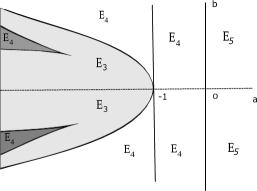
Figure 2. Axiumbilic types $E_{3}$, $E_{4}$ and $E_{5}$ partitioning the plane $(a,b).$

4. Axial Configurations near a Critical Point for a Special Family of Mappings

In this section the axial configuration of the special family of mappings defined by equation (11) near the critical point will be established.

Consider the mapping

(11) $$\alpha^{a}(u,v)=\alpha(u,v)=(u,uv,v^{2},\frac{1}{6}av^{3})$$

and the vector $W=\alpha_{u}\wedge\alpha_{uv}\wedge\alpha_{vv}$.

Define the normal vectors   $\mathbf{N}_{1}=\alpha_{u}\wedge\alpha_{v}\wedge W$ and $\mathbf{N}_{2}=\alpha_{u}\wedge\alpha_{v}\wedge\mathbf{N}_{1}$.

The first fundamental form of $\alpha$ is given by:

(12) $$E= 1+u^{2},\;\;\;\;\;\;F=uv,\;\;\;\;\;\;G=u^{2}+4v^{2}+\frac{1}{2}a^{2}v^{4}$$

The normal vectors are given by:

$$\mathbf{N}_{1}= (-\frac{1}{2}a^{2}v^{4}-4v^{2},4v+\frac{1}{2}a^{2}v^{3},-2u,-auv)$$

$$\mathbf{N}_{2}= (-auv^{3},auv^{2},-au^{2}v-2av^{3}-\frac{1}{4}a^{3}v^{5}-\frac{1}{4}a^{3}v^{7}-2av^{5},$$

$$2u^{2}+8v^{2}+a^{2}v^{4}+a^{2}v^{6}+8v^{4}).$$

The coefficients $\overline{e_{1}}=\langle\alpha_{uu},\mathbf{N}_{1}\rangle$, $\overline{f_{1}}=\langle\alpha_{uv},\mathbf{N}_{1}\rangle$, $\overline{g_{1}}=\langle\alpha_{vv},\mathbf{N}_{1}\rangle$, $\overline{e_{2}}=\langle\alpha_{uu},\mathbf{N}_{2}\rangle$, $\overline{f_{2}}=\langle\alpha_{uv},\mathbf{N}_{2}\rangle$, $\overline{g_{2}}=\langle\alpha_{vv},\mathbf{N}_{2}\rangle$ are given by:

(13) $$\overline{e_{1}}= 0,\;\;\;\overline{f_{1}}=4v+\frac{1}{2}a^{2}v^{3},\;\;\;\overline{g_{1}}=-u(4+a^{2}v^{2})$$

$$\overline{e_{2}}= 0,\;\;\;\overline{f_{2}}=auv^{2},\;\;\;\;\;\;\;\;\;\;\;\;\;\;\overline{g_{2}}=\frac{1}{2}av^{3}(1+v^{2})(8+a^{2}v^{2})$$

From equations (12) and (13) it follows that the functions $\overline{a_{0}}$ and $\overline{a_{1}}$ in equation (6), after multiplication by $-\frac{8}{(1+v^{2})|\mathbf{N}_{1}|^{2}}$, are given by:

$$\overline{a_{1}}= [(24-2a^{2})v^{2}-8]u^{2}+\frac{1}{2}v^{4}[(a^{2}-2a)v^{2}+16-2a][(a^{2}+2a)v^{2}+16+2a]$$

$$\overline{a_{0}}= uv(8+24v^{2}+a^{2}v^{2}+2a^{2}v^{4}).$$

Therefore the differential equation of axial lines in the singular surface is written

(14) $$\overline{{\mathcal{G}}}(u,v,du,dv)= [\overline{a_{0}}G(EG-4F^{2})+\overline{a_{1}}F(2F^{2}-EG)]dv^{4}$$

$$+ [-8\overline{a_{0}}EFG+\overline{a_{1}}E(4F^{2}-EG)]dv^{3}du+$$

$$[ -6\overline{a_{0}}GE^{2}+3\overline{a_{1}}FE^{2}]dv^{2}du^{2}+\overline{a_{1}}E^{3}dvdu^{3}+\overline{a_{0}}E^{3}du^{4}=0,$$

$$\overline{a_{1}}= [(24-2a^{2})v^{2}-8]u^{2}+\frac{1}{2}v^{4}[(a^{2}-2a)v^{2}+16-2a][(a^{2}+2a)v^{2}+16+2a]$$

$$\overline{a_{0}}= uv(8+24v^{2}+a^{2}v^{2}+2a^{2}v^{4}),\;\;E=1+u^{2},\;F=uv,\;G=u^{2}+4v^{2}+\frac{1}{2}a^{2}v^{4}$$

Proposition 3.

Consider the mapping given by equation (11) in the plane $M=\mathbb{R}^{2}$ and its Lie-Cartan variety $\overline{\mathcal{G}}(u,v,du,dv)=0$ defined by equation (14). The projection $\pi:PM\to M$ restricted to $\overline{\mathcal{G}}^{-1}(0)$ is a regular four-fold covering outside the projective line $\pi^{-1}(0)$.

Outside a neighborhood of the vertical direction $(0,[0:1])$, where the variety $\overline{{\mathcal{G}}}^{-1}(0)$ has a degenerate singular point, it is the union of two regular surfaces intersecting transversally along the projective line.

Proof.

As the singular point is of Whitney type it follows that it is isolated and in a punctured neighborhood $U_{0}=U\setminus\{0\}$ of $0$ the map $\alpha$ is an immersion. Below it is shown that there are no axiumbilic points of $\alpha$ in $U_{0}$.

From equation (14) it follows that

$$\overline{a_{1}}(u,v)= [(24-2a^{2})v^{2}-8]u^{2}+\frac{1}{2}v^{4}[(a^{2}-2a)v^{2}+16-2a][(a^{2}+2a)v^{2}+16+2a]$$

$$\overline{a_{0}}(u,v)= uv(8+24v^{2}+a^{2}v^{2}+2a^{2}v^{4})$$

Therefore, $\overline{a_{0}}(u,v)=0$ if only if $u=0$ or $v=0$. As $\overline{a_{1}}(u,0)=-8u^{2}$ and $\overline{a_{1}}(0,v)=\frac{1}{2}v^{4}[(a^{2}-2a)v^{2}+16-2a][(a^{2}+2a)v^{2}+16+2a]$ it follows that there are no axiumbilic in a punctured neighborhood of $0$. ∎

Outside a neighborhood of $(0,[0:1])$ the variety $\overline{\mathcal{G}}=0$ is the union of two regular surfaces which intersect transversally along the projective axis. In Fig. 3 is sketched the topological type of $\overline{\mathcal{G}}=0$ near the critical point $(0,[0:1])$ with a cut along the projective axis when $|a|<8$.

In Fig. 4 is shown the topological type of $\overline{\mathcal{G}}=0$ near the critical point $(0,[0:1])$ when $|a|>8$.

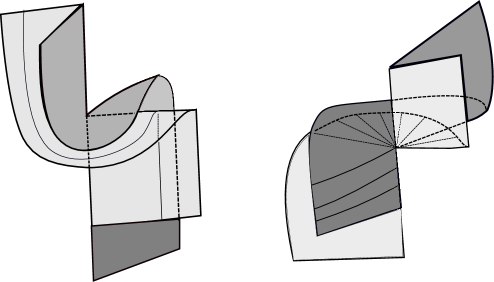
Figure 3. The two sheets of the Lie-Cartan surface $\overline{\mathcal{G}}=0$ over the critical point of the map $\alpha(u,v)=(u,uv,v^{2},a/6v^{3})$ for $|a|<8$, union of two topological cylinders near the critical point $q=0$. Gluing the two pictures (left and right) by juxtaposition along the vertical $q-$axis is recovered the singular surface consisting on two crossing topological cylinders, locally one on the plane of the drawing and the other transversal to it.

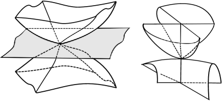
Figure 4. Singular Lie-Cartan surface $\overline{\mathcal{G}}=0$ of the map $\alpha(u,v)=(u,uv,v^{2},a/6v^{3})$. For $|a|>8$ is the union of four topological punctured disks. Three of them are near the singular point, the other has the projective line in its closure.

Proposition 4.

Consider the planar blowing-up $\psi(u,t)=(u,tu)$ around the origin. Then, in $(u,t)$-coordinates, Equation (14) restricted to the a small neighborhood of t-axis has the form:

$$du^{3}[8dt+ut^{3}(2t^{2}+1)(a^{2}+16)du]+0(u^{2})]=0$$

Therefore, the pull-back of the axial configuration restricted to a small neighborhood of the t-axis is as in Figure 5. Three axial lines are almost vertical e one is transversal to axis $t$ and almost horizontal.

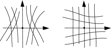
Figure 5. Pull-back of the axial configuration restricted to a small neighborhood of the t-axis.

Proof.

The differential equation (14) restricted to $v=0$ is given by: $-16u^{2}dudv(du-udv)(du+udv)=0$. One axial direction is horizontal $dv=0$, one is vertical $du=0$ and two are almost vertical $\frac{du}{dv}=u$ and $\frac{du}{dv}=-u$.

The proof follows from direct calculations leading to $\psi_{*}(\overline{{\mathcal{G}}})$ as stated. ∎

Proposition 5.

Consider the planar blowing-up $\vartheta(u,v)=(r^{2}\sin\theta,r\cos\theta)$ around the origin. Then, in $(\theta,r)$-coordinates, Equation (14) restricted to the a small neighborhood of the $\theta-$axis in the region $\{r\geq 0\}$ has the form:

(15) $$\vartheta_{*}(\overline{{\mathcal{G}}})= dr^{3}.[2\cos\theta\sin\theta((20-a^{2})\cos^{4}\theta\sin^{2}\theta+4\sin^{4}\theta+(a^{2}-56)\cos^{8}\theta)dr$$

$$+ r[(7a^{2}-384)\cos^{10}\theta+(260-a^{2})\cos^{8}\theta+(-7a^{2}+32)\cos^{6}\theta+(24+2a^{2})\cos^{4}\theta$$

$$- 4\cos^{2}\theta+8]d\theta]+r^{2}.O(r,\theta,dr,d\theta)={\mathcal{E}}_{r}(\theta,r,d\theta,dr)$$

The singular points of ${\mathcal{E}}_{r}(\theta,r,d\theta,dr)$ in the $\theta$-axis are given by

$$2\cos\theta\sin\theta((20-a^{2})\cos^{4}\theta\sin^{2}t+4\sin^{4}\theta+(a^{2}-56)\cos^{8}\theta)=0.$$

Near the $\theta$-axis three axial line fields are almost horizontal and the other is defined by the following differential equation:

(16) $$\omega= 2\cos\theta\sin\theta((20-a^{2})\cos^{4}\theta\sin^{2}\theta+4\sin^{4}\theta+(a^{2}-56)\cos^{8}\theta+r.O(r))dr$$

$$+ r[(7a^{2}-384)\cos^{10}\theta+(260-a^{2})\cos^{8}\theta+(-7a^{2}+32)\cos^{6}\theta+(24+2a^{2})\cos^{4}\theta$$

$$- 4\cos^{2}\theta+8+r.O(r)]d\theta=0$$

Proof.

Direct calculations shows that $\vartheta_{*}({\mathcal{E}})$ is as stated. ∎

Proposition 6.

The differential equation $\omega=0$ given by equation (16) assuming that $|a|\neq\sqrt{56}$ and $|a|\neq 8$ has either eight or twelve singular points in the interval $[0,2\pi)$ with three or five hyperbolic singular points in the interval $(-\frac{\pi}{2},\frac{\pi}{2})$ contained in the $\theta$-axis. See Fig. 6 and Fig. 7.

Moreover,

1. If $|a|<\sqrt{56}$ six singular points are hyperbolic saddles and $(\pm\frac{\pi}{2},0)$ are hyperbolic nodes.

2. If $\sqrt{56}<|a|<8$, eight singular points are hyperbolic saddles and the point s$(\theta,r)=(0,0)$ and $(\pi,0)$ and $(\pm\frac{\pi}{2},0)$ are hyperbolic nodes.

3. If $8<|a|$, ten singular points are hyperbolic saddles and $(\pm\frac{\pi}{2},0)$ are hyperbolic nodes.

Proof.

The singular points of $\omega=0$ are given by

$$r=0,\;\;\;\cos\theta\sin\theta[(20-a^{2})\cos^{4}\theta\sin^{2}\theta+4\sin^{4}\theta+(a^{2}-56)\cos^{8}\theta]=0.$$

Writing this equation using the relations $t=\tan\theta,\;\ \cos\theta=\frac{1}{\sqrt{1+t^{2}}},\;\ \sin\theta=\frac{t}{\sqrt{1+t^{2}}}$ it follows that it is equivalent to:

$$p(t)= t[4t^{8}+8t^{6}-(a^{2}-24)t^{4}-(a^{2}-20)t^{2}+a^{2}-56],$$

$$t= \tan\theta\;\;\;\text{ and}\;\;\;\theta=\pm\frac{\pi}{2}.$$

The polynomial $p(t)$ has the following factorization:

$$p(t)= 4tp{{}_{1}}(t^{2})p{{}_{2}}(t^{2}),$$

$$p{{}_{1}}(t)= t^{2}+t+\frac{5}{2}-\frac{1}{8}\sqrt[2]{a^{4}-56a^{2}+1296},$$

$$p{{}_{2}}(t)= t^{2}+t+\frac{5}{2}+\frac{1}{8}\sqrt[2]{a^{4}-56a^{2}+1296}.$$

The polynomial $p_{1}$ always has two real simple roots, one positive and the other negative.

The polynomial $p_{2}$ has a positive root for $|a|>\sqrt{56}$ and for $|a|=\sqrt{56}$, $p_{2}(0)=0$ and for $|a|<\sqrt{56}$ the roots of $p_{2}$ are negative or complex.

So it follows that:

1. For $|a|<\sqrt{56}$, $\omega=0$ has three singular points in the interval $(-\frac{\pi}{2},\frac{\pi}{2}).$

2. For $|a|>\sqrt{56}$ and $|a|\neq 8$, $\omega=0$ has five singular points in the interval $(-\frac{\pi}{2},\frac{\pi}{2}).$

The differential equation $\omega=0$ has the same solution curves as the vector field $X=\mathbf{P}\frac{\partial}{\partial\theta}+\mathbf{Q}\frac{\partial}{\partial\theta}$, where

(17) $$\mathbf{P}(\theta,r)= 2\cos\theta\sin\theta[(20-a^{2})\cos^{4}\theta\sin^{2}\theta+4\sin^{4}\theta+(a^{2}-56)\cos^{8}\theta+r.O(r)]=P(\theta)+r.O(r)$$

$$\mathbf{Q}(\theta,r)= -r[(7a^{2}-384)\cos^{10}\theta+(260-a^{2})\cos^{8}\theta+(-7a^{2}+32)\cos^{6}\theta+(24+2a^{2})\cos^{4}\theta$$

$$- 4\cos^{2}\theta+8+r.O(r)]=-r[Q(\theta)+r.O(r)]$$

The jacobian of $DX(\theta,0)$ at the singular point $(\theta,0)$, $t=\tan\theta$, is given by: $-P^{\prime}(\theta)Q(\theta)=\frac{1}{(1+t^{2})^{10}}r_{a}t_{a}$, where

$$r_{a}= -[8t^{10}+36t^{8}+(2a^{2}+88)t^{6}+(160-a^{2})t^{4}+(420-9a^{2})t^{2}+a^{2}-64]$$

$$t_{a}= 2[-4t^{10}+12t^{8}+(5a^{2}-64)t^{6}+(2a^{2}-20)t^{4}+(564-12a^{2})t^{2}+a^{2}-56]$$

At $\theta=\pm\frac{\pi}{2}$ the jacobian of $DX(\pm\frac{\pi}{2},0)$ is always equal to $64$ and at $\theta=0$ is given by:$-2(a^{2}-56)(a^{2}-64).$

Evaluation of the resultants of polynomials, abbreviated by res, give that

$$\text{res}(p(t),r_{a},t)= -1073741824(a^{2}-64)(5a^{2}-243)^{2}(a^{2}-36)^{12}$$

$$\text{res}(p(t),t_{a},t)= 549755813888(a^{2}-56)^{5}(5a^{2}-243)^{2}(1296-56a^{2}+a^{4})^{4}$$

The values $a^{2}=36$ and $a^{2}=\frac{243}{5}$ correspond to double complex roots, while $a^{2}=64$ and $a^{2}=56$ correspond to double real roots.

For $|a|>8$ the sign of $r_{a}$ in the roots of $p(t)=0$ is negative, while for $|a|<8$ this sign is negative.

Therefore all singular points of $X$ different from $(0,0)$ are hyperbolic saddles. The point $(0,0)$ is a hyperbolic node for $\sqrt{56}<|a|<8$ and hyperbolic saddle when $|a|<\sqrt{56}$ or $|a|>8$. ∎

Proposition 7.

Consider the planar blowing-up $\vartheta(u,v)=(r^{2}\sin\theta,r\cos\theta)$ around the origin. Then, in $(\theta,r)$-coordinates, the resolution of the axial configuration is as shown in Fig. 6 and Fig. 7.

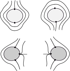
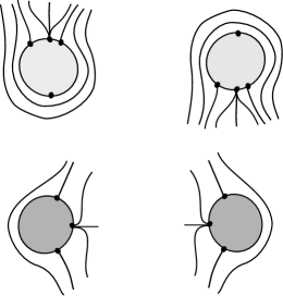
Figure 6. Singular points of index $1/2$. Left, with $|a|<\sqrt{56}$ and Right, with $8>|a|>\sqrt{56}.$

Figure 7. Singular points of index $0$, $|a|>8$. Behavior of the axial configuration in each topological disk.

Proof.

For $a=0$ the map $\alpha(u,v)=(u,uv,v^{2},0)$ is the Whitney stable map. In this case the axial configuration is given by the principal lines and the mean curvature lines. See [2], [10], [12]. The Lie-Cartan variety (14) is a pair of cylinders intersecting along the projective line. See Fig. 3. The resolution is as shown in Fig. 6, left. By continuation, for $|a|<\sqrt{56}$ there are no bifurcation in the resolution. The induced differential equation has three hyperbolic saddles in the interval $(-\frac{\pi}{2},\frac{\pi}{2})$ and other three hyperbolic saddles in the interval $(\frac{\pi}{2},\frac{3\pi}{2})$. The points $(\pm\frac{\pi}{2},0)$ are hyperbolic nodes.

For $\sqrt{56}<|a|<8$ the Lie-Cartan surface is still a pair of cylinders, but the induced differential equation has four hyperbolic saddles in the interval $(-\frac{\pi}{2},\frac{\pi}{2})$ and $\theta=0$ is a hyperbolic node. Also it has four hyperbolic saddles in the interval $(\frac{\pi}{2},\frac{3\pi}{2})$ and the points $(\pm\frac{\pi}{2},0)$ are hyperbolic nodes. See Fig. 6, right.

For $|a|>8$ the Lie-Cartan variety is the union of four topological disks, see Fig. 4 and the induced differential equation has five hyperbolic saddles in the interval $(-\frac{\pi}{2},\frac{\pi}{2})$ and five hyperbolic saddles in the interval $(\frac{\pi}{2},\frac{3\pi}{2})$. The points $(\pm\frac{\pi}{2},0)$ are hyperbolic nodes. See Fig. 7. ∎

Proposition 8.

Consider the map $\alpha(u,v)=(u,uv,v^{2},\frac{1}{6}av^{3})$ which has a Whitney singularity at $(0,0)$.

For $|a|<8$ the axial configuration has index $1/2$ at $(0,0)$ and when $|a|<\sqrt{56}$ the axial configuration is as shown in of Fig. 8 (left) and for $\sqrt{56}<|a|<8$ the axial configuration is as shown in Fig. 8, (right).

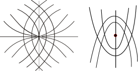
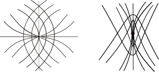
Figure 8. Axial Configurations near a critical point of index $\frac{1}{2}$. Left for $|a|<\sqrt{56}$ and right for $\sqrt{56}<|a|<8$.

For $|a|>8$ the axial configuration has index $0$ at $(0,0)$ and it is as shown in Fig. 9.

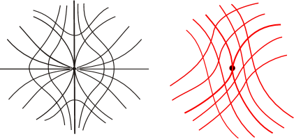
Figure 9. Axial Configurations near a singular point of index $0$ ( $|a|>8$).

Proof.

Follows from Proposition 7 performing the blowing-down of the resolution of the axial lines shown in Figs. 6 and 7. ∎

Proposition 9.

For $\epsilon\neq 0$ small, consider the immersion $\alpha_{\epsilon}(u,v)=(u,uv,v^{2},\epsilon v+\frac{a}{6}v^{3})$. Then it follows that:

$\bullet$ For $|a|\leq 8$ and $\epsilon\neq 0$ the immersion $\alpha_{\epsilon}$ has two axiumbilic points.

$\bullet$ For $a>8$ the immersion $\alpha_{\epsilon}$ has four axiumbilic points when $\epsilon>0$ and no axiumbilic points when $\epsilon<0$.

$\bullet$ For $a<-8$ the immersion $\alpha_{\epsilon}$ has four axiumbilic points when $\epsilon<0$ and no axiumbilic points when $\epsilon>0$.

Moreover, the axial configuration is as described below.

$\bullet$ For $a>8$, two axiumbilic points are of type $E_{3}$ and two are of type $E_{5}$. See Fig. 10, top.

$\bullet$ For $a<-8$, two axiumbilic points are of type $E_{3}$ and two are of type $E_{5}$. See Fig. 10, bottom.

$\bullet$ For $|a|<\frac{15}{2}$ the two axiumbilic points are of type $E_{3}$ and the axial configuration is as shown in Fig. 11, left.

$\bullet$ For $\frac{15}{2}<|a|<8$ the two axiumbilic points are of type $E_{4}$ and the axial configuration is as illustrated in Fig. 11, right.

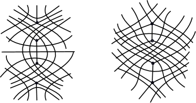
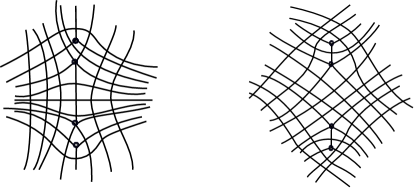
Figure 10. Axial Configurations near axiumbilic points $E_{3}$ and $E_{5}$, branching from index $0$ critical point. Top, $a>8$ and bottom, $a<-8$.

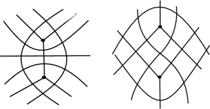
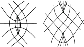
Figure 11. Axial Configurations near axiumbilic points of types $E_{3}$, branching from the index $1/2$ critical point. Left for $|a|<\frac{15}{2}$ and of types $E_{4}$, right for $\frac{15}{2}<|a|<8$.

Proof.

As in equation (14) it follows that

$$\begin{array}[]{lcr}\overline{e_{1}}=0,\;\;\;\overline{f_{1}}=4v+\frac{1}{2}a^{2}v^{3}+a\epsilon v,\;\;\overline{g_{1}}=-u(4+a^{2}v^{2})\\ \overline{e_{2}}=0,\;\;\;\overline{f_{2}}=auv^{2}-2\epsilon u,\;\;\overline{g_{2}}=\frac{1}{2}av^{3}(1+v^{2})(8+a^{2}v^{2})-(8\epsilon+2a\epsilon^{2})(1+v^{2})\end{array}$$

Therefore,

(18) $$\overline{a_{1}}= [(24-2a^{2})v^{2}-8]u^{2}+\frac{1}{2}v^{4}[(a^{2}-2a)v^{2}+16-2a][(a^{2}+2a)v^{2}+16+2a]$$

$$+ 8\epsilon^{4}+16a\epsilon^{3}v^{2}+(8u^{2}-8v^{4}+12a^{2}v^{4}-8+48v^{2})\epsilon^{2}$$

$$+ 4av^{2}(2+a^{2}v^{4}+2u^{2}+20v^{2}+2v^{4})\epsilon$$

$$\overline{a_{0}}= uv[8+24v^{2}+a^{2}v^{2}+2a^{2}v^{4}+2a\epsilon(1+3v^{2})+4\epsilon^{2}].$$

The axiumbilic points of $\alpha_{\epsilon}$ are defined by $\overline{a_{0}}=\overline{a_{1}}=0$.

So, for $\epsilon$ small they are defined by:

$$u^{2}+\epsilon^{2}=0,\;\;v=0$$

$$u =0,\;\;[(2a+a^{2})v^{4}+(-4\epsilon+4a\epsilon+16+2a)v^{2}+4\epsilon^{2}-4\epsilon].$$

$$[ (-2a+a^{2})v^{4}+(4\epsilon+4a\epsilon+16-2a)v^{2}+4\epsilon^{2}+4\epsilon]=0$$

For $\epsilon=0$ it follows that $\frac{1}{2}v^{4}(v^{2}a^{2}-2a+16-2av^{2})(v^{2}a^{2}+2a+16+2av^{2})$.

Solving the equation

$$[(2a+a^{2})v^{4}+(-4\epsilon+4a\epsilon+16+2a)v^{2}+4\epsilon^{2}-4\epsilon]=0$$

with respect to $\epsilon$ it follows that

$$\epsilon= \frac{1}{2}+\frac{1}{2}(1+a)v^{2}+\frac{1}{2}\sqrt{1+(1-4a)v^{4}-(4a+14)v^{2}}=$$

$$= \frac{1}{2}(8+a)v^{2}+(12+8a+a^{2})v^{4}+O(5)=\epsilon_{1}(v)$$

Solving the equation

$$(-2a+a^{2})v^{4}+(4\epsilon+4a\epsilon+16-2a)v^{2}+4\epsilon^{2}+4\epsilon]=0$$

it follows that

$$\epsilon= -\frac{1}{2}-\frac{1}{2}(1+a)v^{2}+\frac{1}{2}\sqrt{1+(4a+1)v^{4}+(4a-14)v^{2}}=$$

$$= \frac{1}{2}(a-8)v^{2}-(12+a^{2}-8a)v^{4}+O(5)=\epsilon_{2}(v).$$

For $a^{2}-64\leq 0$ the two curves $(v,\epsilon_{1}(v))$ and $(v,\epsilon_{2}(v))$ are tangent at $0$ and have even contact of opposite signs.

So, for $\epsilon\neq 0$ there are two axiumbilic points $(0,\pm v_{0}(\epsilon))$ symmetric with respect to the $u$-axis. See Fig. 12, center.

                          

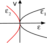
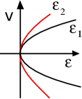
Figure 12. Definition of axiumbilic points (left, $a<-8$), (center, $|a|<8$), (right, $a>8$).

For $a^{2}-64>0$ the two curves $(v,\epsilon_{1}(v))$ and $(v,\epsilon_{2}(v))$ are tangent at $0$ and have even contact of the same signs. See Fig. 12 (left and right). Therefore $\alpha_{\epsilon}$ has four axiumbilic points when $a>8$ and $\epsilon>0$ and also when $a<-8$ and $\epsilon<0$.

Analysis of the axial configuration.

Consider the map $\beta(u,v)=(\overline{a_{0}}(u,v),\overline{a_{1}}(u,v))$, where $\overline{a_{0}}$ and $\overline{a_{1}}$ are given by equation (18).

At an axiumbilic point defined by $\epsilon_{1}(v_{0})=\epsilon$ it follows that $\text{det}D\beta(0,v_{0})=512(8+a)v_{0}^{4}+O(5)$ and for an axiumbilic point defined by $\epsilon_{2}(v_{0})=\epsilon$ it follows that $\text{det}D\beta(0,v_{0})=-512(a-8)v_{0}^{4}+O(5)$.

An axiumbilic point is of type $E_{5}$ when $\text{det}D\beta(0,v_{0})<0$, see [10]. When $\text{det}D\beta(0,v_{0})>0$ the axiumbilic point is of index $1/4$ and the type is not characterized by this sign. This follows from Proposition 2 and 1.

Therefore, for $a>8$ two axiumbilic points defined by $\epsilon_{2}(v_{0})=\epsilon$ are of type $E_{5}$ (index $-\frac{1}{4}$) and for $a<-8$ the two axiumbilic points defined by $\epsilon_{1}(v_{0})=\epsilon$ are of type $E_{5}$.

For $|a|>8$ it will be shown below that they are of type $E_{3}$.

To describe the type of these axiumbilic points consider the linearization of the differential equation (6) of axial lines at an axiumbilic point $(0,v_{0}(\epsilon))$.

Performing the calculations it follows that for $\epsilon=\epsilon_{1}(v_{0})$,

(19) $${\mathcal{E}}_{1}(u,v,du,dv)= A_{4}dv^{4}+A_{3}dudv^{3}+A_{2}dv^{2}du^{2}+A_{1}dvdu^{3}+A_{0}du^{4}=0$$

$$A_{0}(u,v)= [8v_{0}+O(2)]u+0.(v-v_{0})+\ldots$$

$$A_{1}(u,v)= 0.u+[64(8+a)v_{0}^{3}+O(4)](v-v_{0})+\ldots$$

$$A_{2}(u,v)= [-192v_{0}^{3}+0(4)]u+0.(v-v_{0})+\ldots$$

$$A_{3}(u,v)= 0.u-[256(a+8)v_{0}^{5}+O(6)].(v-v_{0})+\ldots$$

$$A_{4}(u,v)= [128v_{0}^{5}+0(6)]u+0.(v-v_{0})+\ldots$$

Further calculations for $\epsilon=\epsilon_{2}(v_{0})$ lead to

(20) $${\mathcal{E}}_{2}(u,v,du,dv)= A_{4}dv^{4}+A_{3}dudv^{3}+A_{2}dv^{2}du^{2}+A_{1}dvdu^{3}+A_{0}du^{4}=0$$

$$A_{0}(u,v)= [8v_{0}+O(2)]u+0.(v-v_{0})+\ldots$$

$$A_{1}(u,v)= 0.u+[64(8-a)v_{0}^{3}+O(4)](v-v_{0})+\ldots$$

$$A_{2}(u,v)= [-192v_{0}^{3}+0(4)]u+0.(v-v_{0})+\ldots$$

$$A_{3}(u,v)= 0.u-[256(8-a)v_{0}^{5}+O(6)].(v-v_{0})+\ldots$$

$$A_{4}(u,v)= [128v_{0}^{5}+0(6)]u+0.(v-v_{0})+\ldots$$

To determine the type of the axiumbilic points $(0,v_{0})$ defined by $\epsilon=\epsilon_{1}(v_{0})$ consider the linear differential equation

$$E_{1}(u,v,du,dv)= 8v_{0}du^{4}+64(8+a)v_{0}^{3}(v-v_{0})du^{3}dv-192v_{0}^{3}udu^{2}dv^{2}$$

$$- 256(a+8)v_{0}^{5}.(v-v_{0})dudv^{3}+128v_{0}^{5}udv^{4}=0.$$

The separatrices of the linear equation are defined by $u=kv$ where $k$ is a root of the polynomial

$$p_{1}(k)=k[k^{4}+8v_{0}^{2}(5+a)k^{2}-16v_{0}^{4}(15+2a)]=0.$$

For $a<-\frac{15}{2}$ the polynomial $p_{1}(k)$ has five real roots while for $a>-\frac{15}{2}$ it has only three real roots.

Analogously, for the axiumbilic points $(0,v_{0})$ defined by $\epsilon=\epsilon_{2}(v_{0})$ consider the differential equation

$$E_{2}(u,v,du,dv)= 8v_{0}du^{4}+64(8-a)v_{0}^{3}(v-v_{0})du^{3}dv-192v_{0}^{3}udu^{2}dv^{2}$$

$$- 256(8-a)v_{0}^{5}.(v-v_{0})dudv^{3}+128v_{0}^{5}udv^{4}=0.$$

The separatrices are defined by $u=kv$ where

$$p_{2}(k)=k[k^{4}+8v_{0}^{2}(a-5)k^{2}+16v_{0}^{4}(2a-15)]=0.$$

For $a>\frac{15}{2}$ the polynomial $p_{2}(k)$ has five real roots, while for $a<\frac{15}{2}$ it has only three real roots.

Therefore, by the classification of axiumbilic points, see [10], for $|a|<\frac{15}{2}$ and $\epsilon>0$ the axiumbilic points $(0,v_{0})$ are defined by $\epsilon=\epsilon_{1}(v_{0})$ and they are all of type $E_{3}$. Also $\frac{15}{2}<|a|<8$ and $\epsilon>0$ all axiumbilic points are defined by $\epsilon=\epsilon_{1}(v_{0})$, see Fig. 12 center, and they are of type $E_{4}$. Analogously, when $\epsilon<0$ the axiumbilic points are defined by $\epsilon=\epsilon_{2}(v_{0})$ and the same analysis and conclusions can be established.

For $a>8$ and $\epsilon>0$ the axiumbilic points defined by $\epsilon=\epsilon_{2}(v_{0})$ are of type $E_{5}$ and the other two defined by $\epsilon=\epsilon_{1}(v_{0})$ have the separatrices given by $p_{1}(k)=0$ which has three real roots for $a>-\frac{15}{2}$. Therefore they are of type $E_{3}$, see Fig. 10, top.

For $a<-8$ and $\epsilon<0$ the axiumbilic points defined by $\epsilon=\epsilon_{1}(v_{0})$ are of type $E_{5}$ and the other two defined by $\epsilon=\epsilon_{2}(v_{0})$ have the separatrices given by $p_{2}(k)=0$ which has three real roots for $a<\frac{15}{2}$. Therefore they are of type $E_{3}$, see Fig. 10, bottom.

The analysis above also follows from Proposition 2, taking into account Fig. 2, illustrating Theorem 1 established in [10]. ∎

5. Concluding Comments

The results established in this work are motivated and provide a continuation of the previous paper by Garcia, Sotomayor and Spindola [3].

The authors believe that these results describe the axial configurations at the generic critical point of a surface mapped into $\mathbb{R}^{4}$, as illustrated in Figures 8 and 9. The results also present a rough description of important partial elements of the transversal, codimension$-1$, bifurcations occurring by the elimination of the critical point.

For the full description of the generic bifurcation phenomenon, a delicate analysis of the breaking of the axiumbilic separatrix connections in Figures 10 and 11 must be carried out.

This connection breaking is due to the presence of coefficients of the third order jet of the mapping omitted in the example treated here.

Ronaldo Garcia
Instituto de Matemática e Estatística
Universidade Federal de Goiás,
CEP 74001–970, Caixa Postal 131
Goiânia, Goiás, Brazil

Jorge Sotomayor
Instituto de Matemática e Estatística
Universidade de São Paulo,
Rua do Matão 1010, Cidade Univeritária, CEP 05508-090,
São Paulo, S. P, Brazil

References

[1]Garcia, R., Sotomayor, J., Lines of Curvature near singular points of implicit surfaces, Bull. Sciences Math., 117 (1993), 313-331.
[2]Garcia, Ronaldo; Gutierrez, Carlos; Sotomayor, Jorge, Lines of principal curvature around umbilics and Whitney umbrellas. Tohoku Math. J. 52 (2000), 163-172.
[3]Garcia, R., Sotomayor, J.; Spindola , F., Axiumbilic Singular Points on Surfaces Immersed in and their Generic Bifurcations,
arXiv:1304.0197v1 [math.DG] 31 Mar 2013.
[4]Gutiérrez, C., Guíñez, V., Simple Umbilic Points on Surfaces Immersed in . Discrete Contin. Dyn. Syst. 9 (2003), 877-900.
[5]Levine, H.T.,
Singularities of Differentiable Mappings, Lect. Notes in Math. 192,
(1971).
[6]Little, J. A., On Singularities of Submanifolds of Higher Dimensional Euclidean Spaces. Ann. Mat. Pura Appl., 83 (1969), 261-335.
[7]Oliver, J. M., On pairs of foliations of a parabolic cross-cap. Qual. Theory Dyn. Syst.10 (2011), 139-166.
[8]Mello, L. F., Mean Directionally Curved Lines on Surfaces Immersed in . Publ. Mat., 47 (2003), 415-440.
[9]Porteous, I. R., Geometric differentiation. For the intelligence of curves and surfaces. Cambridge University Press, Cambridge, (2001).
[10]Sotomayor, J., Garcia, R., Lines of Axial Curvature on Surfaces Immersed in . Diff. Geom. and its Applications. 12 (2000), 253-269.
[11]Sotomayor, J., Garcia, R., Lines of curvature on surfaces, historical comments and recent developments. São Paulo J. Math. Sci.2 (2008), 99-143.
[12]Sotomayor, J., Garcia, R., Differential Equations of Classical Geometry, a Qualitative Theory. Publicações Matemáticas. IMPA. 2009.
[13]Tari, F., On pairs of geometric foliations on a cross-cap. Tohoku Math. J. 59 (2007), 233-258.