Parenclitic networks: a multilayer description of heterogeneous and static data-sets

Abstract

Describing a complex system is in many ways a problem akin to identifying an object, in that it involves defining boundaries, constituent parts and their relationships by the use of grouping laws. Here we propose a novel method which extends the use of complex networks theory to a generalized class of non-Gestaltic systems, taking the form of collections of isolated, possibly heterogeneous, scalars, e.g. sets of biomedical tests. The ability of the method to unveil relevant information is illustrated for the case of gene expression in the response to osmotic stress of Arabidopsis thaliana. The most important genes turn out to be the nodes with highest centrality in appropriately reconstructed networks. The method allows predicting a set of 15 genes whose relationship with such stress was previously unknown in the literature. The validity of such predictions is demonstrated by means of a target experiment, in which the predicted genes are one by one artificially induced, and the growth of the corresponding phenotypes turns out to feature statistically significant differences when compared to that of the wild-type.

PACS: 89.75.-k, 05.45.Tp, 02.10.Ox, 87.18.Vf

Of the different ways of representing a multi-unit system, the one afforded by complex networks is among the most elegant and general. In the last years, complex networks Albert2002 ; Barabasi2004 have provided a valuable framework for the analysis of a wealth of natural and man-made systems, in fields as diverse as, amongst others, genetics, proteomics and metabolomics Barabasi2004 , the study of neurological diseases Bullmore2009 , transportation networks Zanin2013 and the World Wide Web Albert1999 . While graph theory allows characterizing systems as soon as they are identified as an object, it says nothing as to what should be treated as such. Defining boundaries and identifying components of a complex system can be a natural, if not trivial, task as in the case of an ensemble of power grids, for which it is immediately evident what nodes, links and system boundaries are. In other cases, where individual components are well-defined, some relationship, either conceptual, semantic, or functional, e.g. friendship in a social network Wassermann1994 or correlated activity at different brain regions Bullmore2009 ; Bassett2006 , helps segmenting the system from its surroundings.

Often, however, defining what can indeed be treated as a system in the first place, may be highly non trivial. Suppose, for instance, that what one wants to study is a set of biomedical data from different individuals, e.g. various blood tests, which are in essence but a collection of scalar values without any history. Prima facie, such an object study would seem to lack the physical or virtual relationships between elements of the system, which anatomic brain fibres or hyper-links respectively provide for brain tissue and pages of a web site. Nor does it appear to be possible to construct the sort of functional links that one can define when time evolving variables are associated to each node, as e.g. the time evolution of a stock price, or of brain activity in a given region. Therefore, whether and how such a matter should be treated as a unitary system is not obvious. In particular, what would the elements be of such a system and how would internal relationships among them be defined?

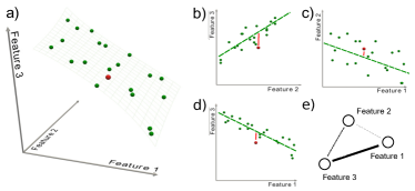
Figure 1: (Color online) Schematic illustration of the parenclitic network reconstruction method. (a) The initial data set, for three features, corresponds to a set of points (green spheres) in a 3-dimensional space. The constraint surface (gray wired surface) represents the overall standard relationship of the class. A generic unlabeled subject is represented by a red sphere. (b,c,d) Data are then projected on each of the three possible planes. The green dashed lines represent the models extracted in each plane. The red points are the positions of the unlabeled subject, and the red lines indicate the distance of the subject from the models. (e) The resulting parenclitic representation is a network where nodes are associated to features, and links are weighted according to the calculated distances (coded, in this Figure, into different line widths).

In this Letter, we introduce a novel way of representing collections of isolated, possibly heterogeneous, scalars as complex networks, wherein the constitutive elements (the nodes) are a group of features characterizing a given subject, and links are weighted according to the deviation between the values of two features and their corresponding typical relationship within a studied population. The result is what we term here a parenclitic network representation, from $\pi\alpha\rho\acute{\varepsilon}\gamma\kappa\lambda\iota\sigma\iota\varsigma$, the Greek term for ”deviation”, originally used by the Greek philosopher Epicurus to designate the spontaneous and unpredictable swerving of free-falling atoms, allowing them to collide Lucretius .

The starting point is a multi-feature description of subjects, e.g. a collection of medical measurements or of genetic expression levels, and a subjects’ affiliation to one or multiple predefined groups. While working with the complete data set may result unfeasible, we consider the projection of the data into all possible plains created by pairs of features. In these plains, different methods (from simple linear correlations, up to more sophisticated data mining techniques) are used to extract reference models for each group. When a new, unlabeled, subject is considered, the deviation between the associated data and such reference models is used to weight the link between the corresponding nodes.

In general terms, consider a set of $n$ systems, or subjects, $\{s_{1},s_{2},\ldots,s_{n}\}$, each one associated to one of $n_{c}$ pre-defined classes - the class of each system will be denoted by $\{c_{1},c_{2},\ldots,c_{n_{c}}\}$. For instance, each subject may represent a person, classified as healthy (or control) or suffering from some disease. Each subject $i$ is, in turn, identified by a vector of $n_{f}$ features $f_{i}=(f^{i}_{1},f^{i}_{2},\ldots,f^{i}_{n_{f}})$, so that each system is represented by a point in a $n_{f}$-dimensional space.

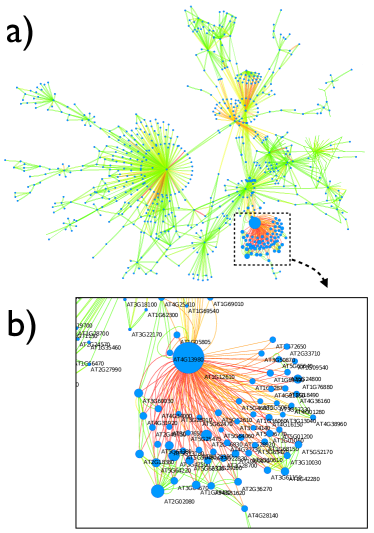
Figure 2: (Color online) Parenclitic network for the response of Arabidopsis thaliana to osmotic stress after 3 h. (a) Pictorial representation of the resulting parenclitic network; for the sake of clarity, links with weight lower than $7$ are not depicted. (b) Magnification of the neighborhood of the most central node, AT1G12610. In both cases, color represents the link weight (from green to red), and node size is associated with the corresponding value of $\alpha$-centrality.

The fundamental ansatz is that each class can be associated to a set of constraints in the features’ space. In other words, for each pairs of features $i$ and $j$, the values corresponding to subjects of a given class $c$ are supposed to lie on a constraint $\tilde{\mathcal{F}}_{i,j}^{c}(f_{i},f_{j})=0$, modeling the relationship expected in that plane for subjects belonging to that class (see Fig. 1 for a schematic illustration). Such reference models can be obtained by several methods, like for instance a polynomial fit, or more generally by a data mining method like Support Vector Machine or Artificial Neural Networks. For each unlabeled subject, a parenclitic network of $n_{f}$ nodes is then constructed where vertices represent the features, and the distance between the subject’s position in the plane of features $i$ and $j$ and the derived model $\tilde{\mathcal{F}}_{i,j}^{c}(f_{i},f_{j})=0$ is used to weight the link between nodes $i$ and $j$ - see the red dot and line in Fig. 1 (b) and the resulting topology illustrated in Fig. 1 (c). Notice that each of the ensuing $\frac{n_{f}(n_{f}-1)}{2}$ links is here a vector of $c$ scalar components, and therefore the arising network is intrinsically a multilayer network, where each layer quantifies the subject deviation from one of the pre-defined classes. Suitable, optimized, thresholding techniques can be used to later transform such a weighted clique into a structured, sparse, network zaninzanin .

The topological characteristics of the parenclitic network can then be used to extract relevant, otherwise inaccessible, information about the system. In particular, atypical or pathological conditions correspond to strongly heterogeneous networks, whereas typical or normative conditions are characterized by sparsely connected networks with homogeneous nodes Zanin2011 . Insofar as a network representation of each instance is constructed with reference to the population to which it is compared, this technique is by its very nature a difference seeker.

While such a graph representation is of general applicability to all systems whose available information is limited to collections of static expressions of features (and it also allows merging different data sources into a single network), in the following we will illustrate its details and prediction power in a specific, relevant, context: the genetic expression of the plant Arabidopsis thaliana under osmotic stress, with the objective of identifying those genes orchestrating the plant’s response under such a stress condition.

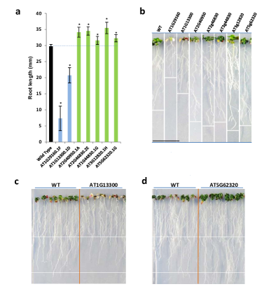
Figure 3: (Color online) In vivo experimental verification of the predictions. (a) Mean root length corresponding to the wild type (WT, black column) and to 7 other transgenic lines in which a specific gene has been knocked out. Whiskers represent the standard deviation corresponding to each group. Asterisks denote groups for which the distribution of root lengths is different with respect to the wild type with a $0.01$ significance level. (b) Photos of one plant of each of the 8 lines, at the end of the full development process. (c) and (d) Photos of two vertical plates where plants are grown. In both cases, the left (right) photos refer to wild phenotypes (to phenotypes developed by the transgenic line).

Data are obtained from the AtGenExpress project Kilian2007 , including expression levels of $22,620$ genes under 8 different abiotic stresses (i.e., cold, heat, drought, osmotic, salt, wounding and UV-B light) and at six different moments of time (30 min, 1 h, 3 h, 6 h, 12 h and 24 h after the onset of stress treatment). Of these, we focus in the following only on the osmotic stress, and the analysis is then performed onto the $n_{f}=1,922$ genes composing the transcription factors of Arabidopsis Guo2005 . While the classical approach considers co-expression networks Clifton2005 , the parenclitic network representation focuses on those pairs of genes whose expressions depart from a reference model. The two methods are therefore strongly complementary: the former focusing on similarities between the evolutions of expression levels through time, the latter concentrating on differences.

In our approach, we create a network for each time step by considering as ”subjects” the statuses of the plant at the other time steps, this way concentrating on those pairs of features whose current relationship deviates from that of all other times. In other words, when analyzing data at time $\tau$, we create the $n_{f}(n_{f}-1)$ reference models $\{\tilde{\mathcal{F}}=0\}$ for the unique class ($c=1$) of those data corresponding to all other time steps, and we generate links according to the distance from that reference.

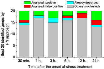
Figure 4: (Color online) Screening of the experimental results. Bars account for the 20 most central genes at each time step. For the six time steps considered, bar colors are coded according to the following stipulations: genes previously considered not to be involved in the plant’s response to osmotic stress, that were respectively experimentally proven to develop (green) or to fail to develop (red) a statistically significant difference in the phenotype with respect to the wild phenotype; (cyan) genes predicted by the parenclitic analysis that were previously associated with the stress response in the Literature; and (gray) previously unknown genes, which could not be tested experimentally.

Precisely, given two gene expression levels $i$ and $j$, we define our reference models by linear regression as $\tilde{f_{j}^{\tau}}=\alpha_{ij}+\beta_{ij}f_{i}^{\tau}$, where $\tilde{f_{j}^{\tau}}$ is the expected value of gene $j$ at time $\tau$, $f_{i}^{\tau}$ the known expression levels of gene $i$, and $\alpha_{ij}$ and $\beta_{ij}$ two free model parameters. These two coefficients are calculated by means of a linear fit of all values corresponding to other time steps, i.e., minimizing the error of the relation $f_{j}^{t\neq\tau}=\tilde{\mathcal{F}}(f_{i}^{t\neq\tau})=\alpha_{ij}+\beta_{ij}f_{i}^{t\neq\tau}$. The distance between the expected (corresponding to the model $\tilde{\mathcal{F}}(f_{i}^{t\neq\tau})$) and the real value of gene $j$ is then used to weight the link connecting nodes $i$ and $j$ in the network. More specifically, the weight of the link is the absolute value of the Z-Score of the distance $\left|{\ \tilde{f_{j}^{\tau}}-f_{j}^{\tau}}\right|$.

As for the identification of the more central nodes (i.e., genes) within each of the six parenclitic networks, we opted for the $\alpha-centrality$ measure, according to which the centrality of a node is a linear combination of the centralities of those to whom it is connected Bonacich2001 . If we define a vector $\mathcal{X}$ of centralities such that its $i^{th}$ component $x_{i}$ is the centrality of the $i$-th node, we have $\lambda x_{i}=\sum\limits_{j}{x_{j}(W_{ij}+\alpha)},\ \ (W+\alpha)\mathcal{X}=\lambda\mathcal{X}$. Here, $W$ is the weight matrix of the network, and $W_{i,j}$ codifies the weight of the link connecting nodes $i$ and $j$. Notice that this is equivalent to an eigenvalue problem, with constant $\alpha$ defining weak connections between all the nodes of the network. In order to have meaningful results, $\alpha$ should be smaller than the spectral radius of $W$.

An example of the obtained networks is shown in Fig. 2. Namely, Fig. 2 (a) depicts the giant component of the network footnote corresponding to 3 h. The color of links accounts for their weights, with green (red) shades indicating low (high) Z-Scores, and the size of nodes is proportional to their $\alpha-centrality$. Remarkably, the resulting network topologies are characterized by a high heterogeneous structure, dominated by a small number of hubs footnote - as can be appreciated from the zoom reported in Fig. 2 (b). Such highly central nodes indicate that, at 3 h., the expression levels of the corresponding genes strongly deviate from the relationships generally established at other times. This suggests that such genes are performing some specific task at this time point, and therefore that they are the main actors in regulating the overall plant response. Thanks to this parenclitic network representation, $15$ new genes, either previously unknown or considered unrelated to the response to osmotic stress, were identified foot , the full list of which is reported in Table 1.

Time step	Gene	Centrality
30 m.	AT1G13300	0.88111
30 m.	AT5G51910	0.729679
30 m.	AT4G23750	0.507826
1 h.	AT1G44830	1.0
1 h.	AT3G12820	0.236686
3 h.	AT2G46830	0.271497
3 h.	AT5G62320	0.177404
3 h.	AT1G29160	0.148112
6 h.	AT4G16610	0.767785
6 h.	AT2G44910	0.689358
12 h.	AT3G61910	0.264721
24 h.	AT1G09540	0.709785
24 h.	AT2G40950	0.551008
24 h.	AT5G62320	0.482752
24 h.	AT5G04410	0.438538

Table 1: Genes previously unknown in the Literature, discovered by the parenclitic network representation, and experimentally proven to develop a statistically significant phenotype. The right most column reports the corresponding centrality values, as normalized to that of the most central node of the 6 networks (the gene AT1G44830).

To confirm these predictions, we further performed an in vivo experiment, in which genes corresponding to the most central nodes of each graph were knocked out, and the appearance of some phenotype was monitored by measuring the length of the root of each plant. Precisely, for the screening of the transcription factors identified by the parenclitic model, the Arabidopsis thaliana inducible lines from Transplanta collection transplanta were used, with the ecotype Columbia (Col-0) as the Wild Type. Each one of the transgenic Arabidopsis lines of the collection expresses a single Arabidopsis transcription factor under the control of the $\beta$-stradiol inducible promoter. In the experiment, seeds from control plants (Col-0) and at least two independent T3 homozygous transgenic lines (Transplanta collection transplanta ) of each transcription factor were sterilized, vernalized for 2 days at $4^{\circ}$C and plated onto Petri dishes containing $\frac{1}{2}$ MS medium Murashige1962 supplemented with $10\mu$M $\beta$-Stradiol. After 5 days, seedlings were transferred to vertical plates containing $\frac{1}{2}$ MS medium supplemented with 300 mM Mannitol, $10\mu$M $\beta$-stradiol and transferred to a growth chamber at $21^{\circ}$C under long-day growth conditions (16/8h light/darkness). After 12 days pictures were taken to record the phenotypes, and root elongation measurements were performed with ImageJ software Abramoff2004 .

As an example, Fig. 3 reports the results obtained with seven transgenic lines, i.e. seven groups of plants in which the expression of one gene was artificially suppressed. Specifically, Fig. 3 (a) reports the mean length of roots for the seven lines, as compared to the expected root length in the wild type (i.e., the plant without genetic modifications, black column). The Figure clearly visualizes the fact that, in all the seven examples, knocking down the corresponding gene leads to a strongly abnormal development of the plant. The complete results of the in vivo screening are summarized in Fig. 4. For each of the six networks analyzed, Fig. 4 reports the number of genes already known to be relevant for the osmotic response of the plant, and the number of previously unknown genes that have been successfully tested.

In conclusion, the parenclitic approach allows a network representation of those data sets lacking both a physical background of connections, and a time-varying nature. Yet, by exploiting the data associated to a set of pre-labeled subjects, and by extracting a set of reference models, it is possible to construct networks whose links represent the presence of deviations from expected relationships. This representation unveils important information on the system, as the identification of key genes regulating the response of the plant Arabidopsis thaliana to osmotic stress, whose role was previously unknown in the literature. Our method generalizes network representation to a very vast number of contexts and data sets previously thought to be outside graph theory’s domain of application.

Authors acknowledge Shlomo Havlin for many fruitful discussion on the subject, as well as the computational resources and assistance provided by CRESCO, the center of ENEA in Portici, Italy.

References

- (1) R. Albert and A.L. Barabási, Rev. Mod. Phys. 74, 47 (2002); S. Boccaletti, V. Latora, Y. Moreno, M. Chavez and D.-U. Hwang, Phys. Rep. 424, 175 (2006).
- (2) A.L. Barabási and Z.N. Oltvai, Nat. Rev. Gen. 5, 101 (2004); R. Guimera and L.A.N. Amaral, Nature 433, 895 (2005).
- (3) E.T. Bullmore and O. Sporns, Nat. Rev. Neurosci. 10, 186 (2009).
- (4) A. Cardillo et al., Nat. Sci. Rep. 3, 1344 (2012).
- (5) R. Albert, H. Jeong and A.L. Barabási, Nature 401, 103 (1999).
- (6) S. Wassermann and K. Faust, Social Networks Analysis (Cambridge University Press, Cambridge, 1994); J. Scott, Social Network Analysis: A Handbook, 2nd ed. (Sage Publications, London, 2000).
- (7) D.S. Bassett and E.D. Bullmore, The neuroscientist 12, 512 (2006); M. Rubinov and O. Sporns, NeuroImage 52, 1059 (2010).
- (8) T. Lucretius Carus, The Way Things Are: The De Rerum Natura, Rolfe Humphries, transl. (Bloomington, Indiana: Indiana University Press, 1968).
- (9) M. Zanin et al., Nat. Sci. Rep. 2, 630 (2012).
- (10) M. Zanin and S. Boccaletti, Chaos 21, 033103 (2011).
- (11) J. Kilian et al., Plant J. 50, 347 (2007).
- (12) A. Guo et al. Bioinformatics 21, 2568 (2005).
- (13) R. Clifton et al., Plant Molecular Biology 58, 193 (2005); L. Mao, J.L. Van Hemert, S. Dash and J.A. Dickerson, BMC Bioinformatics 10, 346 (2009); H. Less, R. Angelovici, V. Tzin and G. Galili, The Plant Cell 23, 1264 (2011).
- (14) P. Bonacich and P. Lloyd, Social Networks 23, 191 (2001).
- (15) While the calculation of centralities was performed over the full weighted clique of distances, for the sake of a better elucidation, in Fig. 2 we have removed those links with weights lower than 7. Therefore, the words hub and giant component are here strictly referring only to the pictorial illustration of the network reported in Fig. 2.
- (16) The names commonly associated to the identified genes listed in Table 1 are: AT1G13300=HRS1; AT5G51910=TCP family transcription factor; AT4G23750=CRF2, Cytokinin response factor 2; AT1G44830=DREB; AT3G12820=MYB10; AT2G46830=ATCCA1, CCA1, Circadian clock associated 1; AT5G62320=MYB99; AT1G29160=COG1; AT4G16610=C2H2-like zinc finger protein; AT2G44910=ATHB-4; AT3G61910=NST2; AT1G09540=MYB61; AT2G40950=ATBZIP17, BZIP17; AT5G62320=MYB99; AT5G04410=ANAC078.
- (17) http://bioinfogp.cnb.csic.es/transplanta_dev/ .
- (18) T. Murashige and F. Skoog, Physiologia plantarum 15, 473 (1962).
- (19) M.D. Abràmoff, P.J. Magalhães and S.J. Ram, Biophotonics International 11, 36 (2004).