Milnor invariants of length $2k+2$ for links with vanishing Milnor invariants of length $\leq k$

Abstract.

J.-B. Meilhan and the second author showed that any Milnor $\overline{\mu}$-invariant of length between $3$ and $2k+1$ can be represented as a combination of HOMFLYPT polynomial of knots obtained by certain band sum of the link components, if all $\overline{\mu}$-invariants of length $\leq k$ vanish. They also showed that their formula does not hold for length $2k+2$. In this paper, we improve their formula to give the $\overline{\mu}$-invariants of length $2k+2$ by adding correction terms. The correction terms can be given by a combination of HOMFLYPT polynomial of knots determined by $\overline{\mu}$-invariants of length $k+1$. In particular, for any 4-component link the $\overline{\mu}$-invariants of length $4$ are given by our formula, since all $\overline{\mu}$-invariants of length $1$ vanish.

1. Introduction

For an ordered, oriented link in the 3-sphere, J. Milnor [7, 8] defined a family of invariants, known as Milnor $\overline{\mu}$-invariants. For an $n$-component link $L$, Milnor invariant is specified by a sequence $I$ of numbers in $\{1,2,\ldots,n\}$ and denoted by $\overline{\mu}_{L}(I)$. The length of the sequence $I$ is called the length of the Milnor invariant $\overline{\mu}_{L}(I)$. It is known that Milnor invariants of length two are just linking numbers. In general, Milnor invariant $\overline{\mu}_{L}(I)$ is only well-defined modulo the greatest common divisor $\Delta_{L}(I)$ of all Milnor invariants $\overline{\mu}_{L}(J)$ such that $J$ is obtained from $I$ by removing at least one index and permuting the remaining indices cyclicly. If the sequence is non-repeated, then this invariant is also link-homotopy invariant and we call it Milnor link-homotopy invariant. Here, the link-homotopy is an equivalence relation generated by self-crossing changes.

In [9], M. Polyak gave a formula expressing Milnor invariant of length 3, and in [6], J-B. Meilhan and the second author generalized it. More precisely, in [6] they showed that any Milnor invariant of length between $3$ and $2k+1$ can be represented as a combination of HOMFLYPT polynomial of knots obtained by certain band sum of the link components, if all Milnor invariants of length $\leq k$ vanish. Their assumption that a link has vanishing Milnor invariants of length $\leq k$ is essential to compute Milnor invariants of length up to $2k+1$ via their formula. In fact, their formula does not hold for length $2k+2$ ([6, Section 7]).

In this paper, we improve their formula to give the Milnor invariants of length $2k+2$ by adding correction terms. Our formula implies that any Milnor invariant of length $2k+2$ can be given by a combination of HOMFLYPT polynomial of knots obtained by certain band sum operations and knots determined by the first non vanishing Milnor invariants, which are Milnor invariants of length $k+1$ (Theorem 1.1). In particular, the Milnor invariants of length $4$ for any link are given by our formula, since all Milnor invariants of length $1$ vanish by the definition (Theorem 1.2).

Recall that the HOMFLYPT polynomial of a knot $K$ is of the form $P(K;t,z)=\sum_{k=0}^{N}P_{2k}(K;t)z^{2k}$ and denote by $P^{(l)}_{0}(K)$ the $l$-th derivative of $P_{0}(K;t)\in\mathbb{Z}[t^{\pm}]$ evaluated at $t=1$. Denote by $(\log P_{0}(K))^{(l)}$ the $l$-th derivative of $\log P_{0}(K;t)$ evaluated at $t=1$. We note that $\log P_{0}(K;t)$ is an additive invariant for knots under the connected sum, since the HOMFLYPT polynomial of knots is multiplicative. In particular, $(\log P_{0}(K))^{(l)}$ is additive. It is known that $P_{0}^{(l)}$ is a finite type invariant of degree $l$ [4]. Since $(\log P_{0}(K))^{(l)}$ is equal to $P_{0}(K)^{(l)}$ plus a sum of products of $P_{0}(K)^{(k)}$’s with $k<l$, $(\log P_{0})^{(l)}$ is an additive finite type knot invariant of degree $l$. We also notice that $(\log P_{0}(K))^{(l)}=P^{(l)}_{0}(K)$ for $l=1,2,3$, since $P_{0}(K;1)=1$ and $P_{0}^{(1)}(K;1)=0$.

Let $L=\bigcup_{i=1}^{n}L_{i}$ be an $n$-component link in $S^{3}$. Let $I=i_{1}i_{2}\ldots i_{m}$ be a sequence of $m$ distinct elements of $\{1,2,\ldots,n\}$. Let $B_{I}$ be an oriented $2m$-gon, and let $p_{j}~{}(j=1,2,\ldots,m)$ denote $m$ mutually disjoint edges of $\partial B_{I}$ according to the boundary orientation. Suppose that $B_{I}$ is embedded in $S^{3}$ such that $B_{I}\cap L=\bigcup_{j=1}^{m}p_{j}$, and such that each $p_{j}$ is contained in $L_{i_{j}}$ with opposite orientation. We call such a disk an I-fusion disk for $L$. For any subsequence $J$ of $I$, we define the oriented knot $L_{J}$ as the closure of $\left((\bigcup_{i\in\{J\}}L_{i})\cup\partial B_{I}\right)\setminus\left((\bigcup_{i\in\{J\}}L_{i})\cap\partial B_{I}\right)$, where $\{J\}$ is the subset of $\{1,2,\ldots,n\}$ formed by all indices appearing in the sequence $J$.

Given a sequence $I$ of elements of $\{1,2,\ldots,n\}$, the notation $J<I$ will be used for any subsequence $J$ of $I$, possibly empty or equal to $I$ itself, and $|I|$ will denote the length of the sequence $I$.

Theorem 1.1.

Let $L$ be an $n$-component link in $S^{3}$ ($n\geq 4$) with vanishing Milnor link-homotopy invariants of length $\leq k$. Then for any sequence $I$ of length $2k+2$ of elements of $\{1,2,\ldots,n\}$ without repeated number and for any $I$-fusion disk for $L$, we have

$$\overline{\mu}_{L}(I)\equiv-\frac{1}{(2k+1)!2^{2k+1}}\sum_{J<I}(-1)^{|J|}(\log P_{0}(L_{J}))^{(2k+1)}-\delta_{L}(I)\pmod{\Delta_{L}(I)},$$

where $\delta_{L}(I)$ is an invariant of $L$ that determined by Milnor invariants for length-$(k+1)$ subsequences of $I$ which is defined in Subsection 2.5.

With the same assumption as in Theorem 1.1, the same formula but $\delta_{L}(I)=0$ holds for a sequence $I$ with $3\leq|I|\leq 2k+1$ [6].

We also give the case of 4-component links more clearly.

Theorem 1.2.

Let $L$ be a 4-component link in $S^{3}$. Then for any sequence $I=i_{1}i_{2}i_{3}i_{4}$ of distinct elements of $\{1,2,3,4\}$ and for any $I$-fusion disk for $L$, we have

$$\overline{\mu}_{L}(I)\equiv-\frac{1}{48}\sum_{J<I}(-1)^{|J|}P^{(3)}_{0}(L_{J})-\frac{1}{2}x_{i_{1}i_{3}}x_{i_{2}i_{4}}(x_{i_{1}i_{3}}+x_{i_{2}i_{4}}-1)\pmod{\Delta_{L}(I)},$$

where $x_{ij}$ is the linking number of $i$-th component and $j$-th component of $L$.

Remark 1.3.

We note that $x_{ij}$ is divisible by $\Delta_{L}(I)$ if $ij$ is a subsequence of $I$. Hence the correction term $\frac{1}{2}x_{i_{1}i_{3}}x_{i_{2}i_{4}}(x_{i_{1}i_{3}}+x_{i_{2}i_{4}}-1)$ vanishes up to modulo $\Delta_{L}(I)$ if either $x_{i_{1}i_{3}}$ or $x_{i_{2}i_{4}}$ is even.

Remark 1.4.

We can generalize Theorem 1.1 and Theorem 1.2 about all repeated sequences by the same arguments as those in [6, Introduction]. That is, we have formulae for not only Milnor link-homotopy invariants but also Milnor isotopy invariants.

2. Preliminary

2.1. String link

Let $n$ be a positive integer, and let $D^{2}\subset\mathbb{R}^{2}$ be the unit disk equipped with $n$ marked points $x_{1},x_{2},\ldots,x_{n}$ in its interior, lying in the diameter on the $x$-axis of $\mathbb{R}^{2}$. An $n$-string link (or $n$-component string link) is the image of a proper embedding $\sqcup_{i=1}^{n}[0,1]_{i}\rightarrow D^{2}\times[0,1]$ of the disjoint union $\sqcup_{i=1}^{n}[0,1]_{i}$ of $n$ copies of $[0,1]$ in $D^{2}\times[0,1]$, such that for each $i$ the image of $[0,1]_{i}$ runs from $(x_{i},0)$ to $(x_{i},1)$. Each string of an $n$-string link is equipped with an (upward) orientation. The $n$-string link $\{x_{1},x_{2},\ldots,x_{n}\}\times[0,1]$ in $D^{2}\times[0,1]$ is called the trivial $n$-string link and denoted by ${\bf 1}_{n}$. Let $y_{1},y_{2},\ldots,y_{n}$ be points in $\partial D^{2}$ in Figure 4, $p_{i}=x_{i}y_{i}~{}(i=1,2,\ldots,n)$ and $q_{j}=y_{j}x_{j+1}~{}(j=1,2,\ldots,n-1)$ segments, and $q_{n}$ an arc in $D^{2}$ connecting $y_{n}$ and $x_{1}$ such that $\bigcup_{i=1}^{n}(p_{i}\cup q_{j})$ bounds the shaded disk in Figure 4. Then for an $n$-string link $l$, the knot

$$l\cup\left(\bigcup_{i=1}^{n}\Bigl{(}(p_{i}\times\{1\})\cup(y_{i}\times[0,1])\cup(q_{i}\times\{0\})\Bigr{)}\right)$$

is called the closure knot of $l$. Note that the link

$$l\cup\left(\bigcup_{i=1}^{n}\Bigl{(}p_{i}\times\{0,1\}\cup y_{i}\times[0,1]\Bigl{)}\right)$$

is the closure $\hat{l}$ of $l$ in the usual sense.

The set of isotopy classes of $n$-string links fixing the endpoints has a monoid structure, with composition given by the stacking product and with the trivial $n$-string link ${\bf 1}_{n}$ as unit element. Given two $n$-string links $L$ and $L^{\prime}$, we denote their product by $L\times L^{\prime}$, which is obtained by stacking $L^{\prime}$ above $L$ and reparametrizing the ambient cylinder $D^{2}\times[0,1]$.

2.2. Clasper

Clasper is defined by K. Habiro [2]. Here we define only tree clasper. For a general definition of clasper, we refer the reader to [2].

Let $L$ be a (string) link. A disk $T$ embedded in $S^{3}$ (or $D^{2}\times[0,1]$) is called a tree clasper for $L$ if it satisfies the following three conditions:

1. $T$ is decomposed into disks and bands, called edges, each of which connects two distinct disks.

2. The disks have either 1 or 3 incident edges. We call a disk with 1 incident edge a leaf.

3. $T$ intersects $L$ transversely, and the intersections are contained in the union of the interiors of the leaves.

Throughout this paper, the drawing convention for claspers are those of [2, Figure 7], unless otherwise specified.

The degree of a tree clasper $T$ is defined as the number of leaves minus 1. A tree clasper of degree $k$ is called a $C_{k}$-tree. A tree clasper for a (string) link $L$ is simple if each of its leaves intersects $L$ at exactly one point. Let $T$ be a simple tree clasper for an $n$-component (string) link $L$. The index of $T$ is the collection of all integers $i$ such that $T$ intersects the $i$-th component of $L$.

Given a $C_{k}$-tree $T$ for a (string) link $L$, there is a procedure to construct a framed link $\gamma(T)$ in a regular neighborhood of $T$. Surgery along T means surgery along $\gamma(T)$. Since there exists an orientation-preserving homeomorphism, fixing the boundary, from the regular neighborhood $N(T)$ of $T$ to the manifold $N(T)_{T}$ obtained from $N(T)$ by surgery along $T$, surgery along $T$ can be regarded as a local move on $L$. We say that the resulting link $L_{T}$ is obtained from $L$ by surgery along $T$. For example, surgery along a simple $C_{k}$-tree is a local move as illustrated in Figure 1.

Similarly, for a disjoint union of trees $T_{1}\cup\ldots\cup T_{m}$ for $L$, we can define $L_{T_{1}\cup\ldots\cup T_{m}}$ as a link obtained by surgery along $T_{1}\cup\ldots\cup T_{m}$. We often regard $L\cup T_{1}\cup\ldots\cup T_{m}$ as $L_{T_{1}\cup\ldots\cup T_{m}}$.

The $C_{k}$-equivalence is an equivalence relation on (string) links generated by surgeries along $C_{k}$-tree claspers and isotopies. We use the notation $L{\sim}_{C_{k}}L^{\prime}$ for $C_{k}$-equivalent (string) links $L$ and $L^{\prime}$.

2.3. Linear trees and planarity

For $k\geq 3$, a $C_{k}$-tree $T$ having the shape of the tree clasper in Figure 1 is called a linear $C_{k}$-tree. The left-most and right-most leaves of $T$ in Figure 1 are called the ends of $T$.

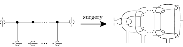
Figure 1. Surgery along a simple tree.

Now suppose that $T$ is a linear $C_{k}$-tree for some knot $K$, and denote its ends by $f$ and $f^{\prime}$. Then the remaining $k-1$ leaves of $T$ can be labeled from $1$ to $k-1$, by travelling along the boundary of the disk $T$ from $f$ to $f^{\prime}$ so that all leaves are visited. We say that $T$ is planar if, when traveling along $K$ from $f$ to $f^{\prime}$, either following or against the orientation, the labels of the leaves met successively are strictly increasing.

Lemma 2.1.

([6, Lemma 3.2]) Let $T$ be a non-planar linear tree clasper for a knot $K$. Then $P_{0}(K_{T};t)=P_{0}(K;t)$.

2.4. Presentation of link-homotopy classes for string links

Let $\mathcal{M}_{k}$ denote the set of all sequences $m_{0}m_{1}\ldots m_{k}$ of $k+1$ non-repeating integers from $\{1,2,\ldots,n\}$ such that $m_{0}<m_{l}<m_{k}$ for $1\leq l\leq k-1$. Let $i_{0}i_{1}\ldots i_{k}$ be a subsequence of $12\cdots n$, and let $a_{M}$ be a permutation of $\{i_{1},i_{2},\ldots,i_{k-1}\}$. Then $M=i_{0}a_{M}(i_{1})\ldots a_{M}(i_{k-1})i_{k}$ is in $\mathcal{M}_{k}$ and all elements of $\mathcal{M}_{k}$ can be realized in this way. Let $T_{M}$ be the simple linear $C_{k}$-tree for ${\bf 1}_{n}$ as illustrated in Figure 2, where    $a_{M}$    is the unique positive $k$-braid which defined the permutation $a_{M}$ and such that every pair of strings crosses at most one. In the figure, we also implicitely assume that all edges of $T_{M}$ overpass all components of ${\bf 1}_{n}$. Let $T^{-1}_{M}$ be the $C_{k}$-tree obtained from $T_{M}$ by inserting a negative half-twist in the $*$ marked edge in Figure 2. We remark that a ‘positive’ half twist is chosen instead of a ‘negative’ one in [6]. Here we choose negative one for a technical reason for the proof of Theorem 1.2.

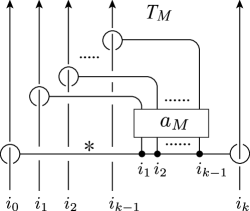
Figure 2. The $C_{k}$-trees $T_{M}$ and ${T}^{-1}_{M}$

Denote respectively by $V_{M}$ and $V_{M}^{-1}$ the $n$-string links obtained from ${\bf 1}_{n}$ by surgery along $T_{M}$ and ${T}^{-1}_{M}$. The following theorem is stated in [6] as a slight modified version of Theorem 4.3 in [10].

Theorem 2.2.

([10, Theorem 4.3],[6, Theorem 4.1]) Any $n$-string link $l$ is link-homotopic to string link $l_{1}\times l_{2}\times\cdots\times l_{n-1}$, where

$$l_{i}=\prod_{M\in\mathcal{M}_{i}}V_{M}^{x_{M}}\textrm{ , where }\quad x_{M}=\left\{\begin{array}[]{ll}\mu_{l}(M)&\text{ if }i=1\\ \mu_{l}(M)-\mu_{l_{1}l_{2}\ldots l_{i-1}}(M)&\text{ if }i\geq 2.\\ \end{array}\right.$$

Here, in the product $\prod_{M\in\mathcal{M}_{i}}V_{M}^{x_{M}}$, the string link $V_{M}^{x_{M}}$ appears in the lexicographic order of $\mathcal{M}_{i}$.

2.5. The correction term

Let $K_{M}^{x}$ and $K_{M,N}^{x,y}$ denote the knot closures of the string links $V^{x}_{M}$ and $V_{M}^{x}\times V_{N}^{y}$ respectively, where $x$ and $y$ are integers, and $M$ and $N$ are subsequences of $12\ldots n$.

Let $I=i_{1}i_{2}\ldots i_{2k+2}$ be a sequence of $\{1,2,\ldots,n\}$ without repeated number. Let $\varphi_{I}$ be a bijection from $\{1,2,\ldots,2k+2\}$ to $\{i_{1},i_{2},\ldots,i_{2k+2}\}$ which sends any $j$ to $i_{j}$. Let $\mathcal{S}$ be the set of pairs $(M,M^{\prime})$ such that $M$ and $M^{\prime}$ are non-successive subsequences of $12\ldots(2k+2)$ with length $k+1$, $1<M$ and $\{M\}\cap\{M^{\prime}\}=\emptyset$. Then for a link $L$ with vanishing Milnor link-homotopy invariants of length $\leq k$, $\delta_{L}(I)$ is defined by

$$-\frac{1}{(2k+1)!2^{2k+1}}\sum_{(M,M^{\prime})\in\mathcal{S}}\left(\log\frac{P_{0}\left(K_{M,M^{\prime}}^{\overline{\mu}_{L}(\varphi_{I}(M)),\overline{\mu}_{L}(\varphi_{I}(M^{\prime}))}\right)}{P_{0}\left(K_{M}^{\overline{\mu}_{L}(\varphi_{I}(M))}\right)P_{0}\left(K_{M^{\prime}}^{\overline{\mu}_{L}(\varphi_{I}(M^{\prime}))}\right)}\right)^{(2k+1)},$$

where $\varphi_{I}(m_{1}m_{2}\ldots m_{k+1})$ means the sequence $\varphi_{I}(m_{1})\varphi_{I}(m_{2})\ldots\varphi_{I}(m_{k+1})$ for a sequence $m_{1}m_{2}\ldots m_{k+1}$. We note that the Milnor invariants of length $k+1$ for $L$ are integer valued invariants and that they are given by linear combinations of $P_{0}^{(k)}$’s by [6, Theorem 1.2]. We also note that $\delta_{L}(I)$ is a link-homotopy invariant of $L$.

Example 2.3.

Let $I=i_{1}i_{2}i_{3}i_{4}$ be a sequence of $\{1,2,3,4\}$ without repeated number. Then $\mathcal{S}$ consists of a single pair $(13,24)$ of non-successive subsequences of $1234$ and

$$\delta_{L}(I)=-\frac{1}{3!2^{3}}\left(\log\frac{P_{0}\left(K_{13,24}^{\overline{\mu}_{L}(i_{1}i_{3}),\overline{\mu}_{L}(i_{2}i_{4})}\right)}{P_{0}\left(K_{13}^{\overline{\mu}_{L}(i_{1}i_{3})}\right)P_{0}\left(K_{24}^{\overline{\mu}_{L}(i_{2}i_{4})}\right)}\right)^{(3)}.$$

2.6. Calculus of claspers for parallel claspers

We shall need the following lemma for parallel tree claspers which is given in [6]. For a positive integer $m$, an $m$-parallel tree means a family of $m$ parallel copies of a tree clasper.

Lemma 2.4.

([6, Lemma 2.2]) Let $m$ be a positive integer. Let $T$ be an $m$-parallel $C_{k}$-tree for a (string) link $L$, and $T^{\prime}$ be a $C_{k^{\prime}}$-tree for $L$. Here $T$ and $T^{\prime}$ are disjoint.
(1) (Leaf slide) Let $\widetilde{T}\cup\widetilde{T^{\prime}}$ be obtained from $T\cup T^{\prime}$ by sliding a leaf $f^{\prime}$ of $T^{\prime}$ over $m$ parallel leaves of $T$ (see Figure 3 (1)). Then, $L_{T\cup T^{\prime}}$ is ambient isotopic to $L_{\widetilde{T}\cup\widetilde{T^{\prime}}\cup Y\cup C}$, where $Y$ denotes the $m$ parallel copies of a $C_{k+k^{\prime}}$-tree obtained by inserting a vertex $v$ in the edge $e$ of $T$ and connecting $v$ to the edge incident to $f^{\prime}$ as shown in Figure 3 (1) and where $C$ is a disjoint union of $C_{k+k^{\prime}+1}$-trees for $L$.
(2) (Edge crossing change) Let $\widetilde{T}\cup\widetilde{T^{\prime}}$ be obtained from $T\cup T^{\prime}$ by passing an edge of $T^{\prime}$ across $m$ parallel edges of $T$ (see Figure 3 (2)). Then, $L_{T\cup T^{\prime}}$ is ambient isotopic to $L_{\widetilde{T}\cup\widetilde{T^{\prime}}\cup H\cup C^{\prime}}$, where $H$ denotes the $m$ parallel copies of a $C_{k+k^{\prime}+1}$-tree obtained by inserting a vertices in both edges, and connecting them by an edge as shown in Figure 3 (2) and where $C^{\prime}$ is a disjoint union of $C_{k+k^{\prime}+2}$-trees for $L$.

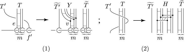
Figure 3. Leaf slide and edge crossing change involving parallel trees

Remark 2.5.

Leaf slides between $C_{k}$-trees for ${\bf 1}_{n}$ with the same index can be realized by link-homotopy, since it is realized by surgery along trees intersecting some component of ${\bf 1}_{n}$ more than twice and since a surgery along such trees is realized by link-homotopy [1, Lemma 1.2]. Hence, in Subsection 2.4, $V_{M}^{x_{M}}$ is link-homotopic to $({\bf 1}_{n})_{T_{M}^{x_{M}}}$, where $T_{M}^{x_{M}}$ is $|x_{M}|$ parallel copies of $T_{M}^{x_{M}/|x_{M}|}$. Note that $V_{M}^{x_{M}}=({\bf 1}_{n})_{T_{M}^{x_{M}}}$ if $x_{M}\geq 0$.

3. Proof of Theorem 1.1

Our strategy of the proof is similar to that in [6, Proof of Theorem 1.1]. In fact, we will use terms ‘good position’ and ‘balanced’ for trees which are defined in [6, Proof of Theorem 1.1] and deform, up to $C_{n}$-equivalence, a balanced set of trees with keeping it balanced as well. The big difference is that we have to treat $C_{k}$-trees $(n=2k+2)$ while they did not need to do. We will repeat same arguments as [6, Proof of Theorem 1.1] part way. We remark that a finite type invariant of degree $\leq n-1$ is an invariant of $C_{n}$-equivalence [2], in particular $\log(P_{0}(K))^{(n-1)}$ is an additive invariant of $C_{n}$-equivalence.

Let $L=\bigcup_{i=1}^{n}L_{i}$ be an $n$-component link in $S^{3}$. Let $I$ be a sequence of $2k+2$ distinct elements of $\{1,2,\ldots,n\}$. It is sufficient to consider here the case $2k+2=n$, because, if $2k+2<n$, we have that $\overline{\mu}_{L}(I)=\overline{\mu}_{\bigcup_{i\in\{I\}}L_{i}}(I)$. We may further assume that $I=12\ldots n$ without loss of generality. Indeed, for any permutation $I^{\prime}$ of $12\ldots n$, we have that $\overline{\mu}_{L}(I^{\prime})=\overline{\mu}_{L^{\prime}}(12\ldots n)$, where $L^{\prime}$ is obtained from $L$ by reordering the components appropriately.

Let $B_{I}$ be an $I$-fusion disk for $L$. Up to isotopy, we may assume that the $2n$-gon $B_{I}$ lies in the unit disk $D^{2}$ as shown in Figure 4, where the edges $p_{j}$ ($j=1,2,\ldots,n$) are defined by $p_{j}=x_{j}y_{j}$. We may furthermore assume that $L\cup B_{I}$ lies in the cylinder $D^{2}\times[0,1]$, such that $B_{I}\subset(D^{2}\times\{0\})$, and such that

$$L\cap\partial(D^{2}\times[0,1])=\bigcup_{j=1}^{n}\Bigl{(}(p_{j}\times\{0,1\})\cup(\{y_{j}\}\times[0,1])\Bigr{)}.$$

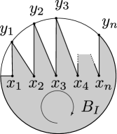
Figure 4. The $2n$-gon $B_{I}$ lying in the unit disk $D^{2}$.

Then, we obtain an $n$-string link $\sigma$ whose closure $\hat{\sigma}$ is the link $L$, by setting

$$\sigma:=\overline{L\setminus(L\cap\partial(D^{2}\times[0,1]))}.$$

For an $n$-string link $\sigma=\bigcup_{i=1}^{n}\sigma_{i}$ and for a subsequence $J$ of $I=12\ldots n$, we denote by $\sigma(J)$ the knot

$$\overline{\biggl{(}\Bigl{(}\bigcup_{j\in\{J\}}\hat{\sigma}_{j}\Bigr{)}\cup\partial B_{I}\biggr{)}\setminus\biggl{(}\Bigl{(}\bigcup_{j\in\{J\}}\hat{\sigma}_{j}\Bigr{)}\cap\partial B_{I}\biggr{)}}.$$

We note that the knot $\sigma(I)$ is equal to the closure knot of $\sigma$ defined in Subsection 2.1.

Let $\sigma$ be the $n$-string link with the closure $L$ defined as above. By combining Theorem 2.2, Remark 2.5, and the assumption that Milnor link-homotopy invariants of length $\leq k$ vanish, $\sigma$ is link-homotopic to $l_{k}\times\cdots\times l_{2k+1}$, where $l_{i}=\prod_{M\in\mathcal{M}_{i}}({\bf 1}_{n})_{T_{M}^{x_{M}}}$. Therefore there is a disjoint union $R_{1}$ of simple $C_{1}$-trees whose leaves intersect a single component of $l_{k}\times\cdots\times l_{2k+1}$ such that $R_{1}$ is disjoint from $\bigcup_{i=k}^{2k+1}\bigcup_{M\in\mathcal{M}_{i}}T_{M}^{x_{M}}$ and

$$\sigma=(l_{k}\times\cdots\times l_{2k+1})_{R_{1}}.$$

Set

$$G:=\bigcup_{i=k}^{2k+1}\left(\bigcup_{M\in\mathcal{M}_{i}}T_{M}^{x_{M}}\right),$$

then we have

$$\sigma=({\bf 1}_{n})_{G\cup R_{1}}.$$

Moreover, by combining Lemmas 4.3 and 4.4 in [6], we have the following:

(3.1) $$\overline{\mu}_{L}(I)\equiv x_{I}~{}\pmod{\Delta_{L}(I)},$$

and

(3.2) $$\Delta_{L}(I)=\gcd\{x_{M}\mid M<I,M\neq I\}.$$

A tree for ${\bf 1}_{n}$ is said to be in good position if each component of ${\bf 1}_{n}$ underpasses all edges of the tree. Note that each tree of $G$ is in good position. On the other hand, a tree of $R_{1}$ may not be in good position. We now replace $R_{1}$ with some trees with good position up to $C_{n}$-equivalence. By [2, Proposition 4.5], we have

$$({\bf 1}_{n})_{G\cup R_{1}}\sim_{C_{n}}({\bf 1}_{n})_{G\cup R},$$

where $R$ is a disjoint union of simple trees for ${\bf 1}_{n}$ in good position and intersecting some component of ${\bf 1}_{n}$ more than once.

It follows from Lemma 2.1 that for any $J<I$,

$$P_{0}(({\bf 1}_{n})_{G\cup R}(J))=P_{0}(({\bf 1}_{n})_{\widetilde{G}\cup R}(J)),$$

where $\widetilde{G}$ is obtained from $G$ by eliminating non-planar trees for $({\bf 1}_{n})(I)$. That is,

$$\widetilde{G}=\bigcup_{i=k}^{2k+1}\left(\bigcup_{M\in\mathcal{M}_{i},M<I}T_{M}^{x_{M}}\right).$$

Here, since $\Delta_{L}(I)$ divides all $x_{M}$ with $M<I$ and $M\neq I$ by (3.2), we assume that each $T_{M}^{x_{M}}$ is a disjoint union of $\Delta_{L}(I)$ parallel copies of $T_{M}^{x_{M}/|x_{M}|}$.

We now define the weight of a tree $t$ for the trivial knot as a subset of $\{1,2,\ldots,n\}$ and denote it by $w(t)$. A disjoint union $g_{1}\cup\ldots\cup g_{s}$ of $s$ trees (possibly parallel) for the trivial knot $U$ is balanced if each tree has a weight such that

$$({\bf 1}_{n})_{\widetilde{G}\cup R}(J)\sim_{C_{n}}U_{\left(\bigcup_{w(g_{i})\subset\{J\}}g_{i}\right)},$$

for any $J<I$.

For the knot $({\bf 1}_{n})_{\widetilde{G}\cup R}(I)$, we may think of $\widetilde{G}\cup R$ as trees $F$ for the trivial knot $U(=({\bf 1}_{n})(I))$. We assign the index of each tree of $F$ as weight. Here we recall that the index of a tree for a (string) link is the collection of all integers $i$ such that the tree intersects the $i$-th component of the (string) link. We may assume that each tree with index $\subset\{J\}$ is also a tree for $({\bf 1}_{n})(J)$. Then it is obvious that for any $J<I$

$$({\bf 1}_{n})_{\widetilde{G}\cup R}(J)=(({\bf 1}_{n})(J))_{\left(\bigcup_{w(g)\subset\{J\}}g\right)},$$

where $\bigcup_{w(g)\subset\{J\}}g$ means the union of trees $g$ of $F$ with weight $\subset\{J\}$. Since $\widetilde{G}\cup R$ is in good position, $(({\bf 1}_{n})(J))_{\left(\bigcup_{w(g)\subset\{J\}}g\right)}$ and $U_{\left(\bigcup_{w(g)\subset\{J\}}g\right)}$ have a common diagram in $D^{2}\times\{0\}$, and hence they are ambient isotopic. In particular $F$ is balanced.

Remark 3.1.

When we perform a leaf slide or an edge crossing change between two trees in a balanced union of trees as in Lemma 2.4, we assign the union of weights as weight to each of new trees. More precisely, in Lemma 2.4 (1) (resp. (2)), we assign the weights $w(T)$ and $w(T^{\prime})$ to $\widetilde{T}$ and $\widetilde{T^{\prime}}$ respectively, and assign the union $w(T)\cup w(T^{\prime})$ to $Y$ (resp. $H$) and each connected component of $C$ (resp. $C^{\prime}$). We note that the union of resulting trees is also balanced.

So far, the proof is the same as [6, Proof of Theorem 1.1]. In [6], they deform $F$ into a balanced union of ‘localized’ tree for the trivial knot $U$ up to $C_{n}$-equivalence. But in that case, there are no $C_{k}$-trees $(n=2k+2)$. The main difficulty of our proof is how to treat such $C_{k}$-trees. In the following, we first deform $F$ into a balanced union of ‘separated’ trees for $U$ except for $C_{k}$-trees, and then deform the $C_{k}$-trees into suitable shape. Here ‘localized’ implies ‘separated’. We use ‘separated’ instead of ‘localized’, since we notice that we do not need to such a strong condition as ‘localized’. So we also slightly modify [6, Proof of Theorem 1.1] in this sense.

For ${M\in{\mathcal{M}}_{i}}~{}(i=k,\ldots,2k+1)$, we denote by $t_{M}^{\pm 1}$ the tree of $F$ which corresponds to $T_{M}^{\pm 1}$ of $\widetilde{G}$. Set

$$d:=\bigcup_{M\in{\mathcal{M}}_{k},M<I}t^{x_{M}}_{M},~{}\text{and}~{}D:=U_{d}.$$

Then $U_{F}$ is obtained from $D$ by surgery along the trees of $F\setminus d$. By using leaf slides and edge crossing changes, we will deform, up to $C_{n}$-equivalence, $F$ into a balanced set of ‘separated’ trees for $U$ with fixing $d$ as in claim below.

Claim 3.2.

The knot $U_{F}$ is $C_{n}$-equivalent to the connected sum $D\#(\#_{J<I}C^{J})$ of knots $D$ and $C^{J}~{}(J<I)$, where $C^{J}$ is a knot obtained from the trivial knot by surgery along a disjoint union $F_{J}$ of trees with weight $\{J\}$ and the set $d\cup(\bigcup_{J<I}F_{J})$ is balanced. Moreover $F_{I}$ consists of the parallel tree $t_{I}^{x_{I}}$ and $\Delta_{L}(I)$-parallel $C_{2k+1}$-trees.

We define that a tree has full weight if the degree of the tree plus one is equal to the number of weight of the tree. We define that a tree is repeated if the degree of the tree is more than or equal to the number of weight of the tree.

Proof.

We take mutually disjoint 3-balls $N_{J}~{}(\{J\}\in 2^{\{1,2,\ldots,n\}})$ such that $(N_{J},N_{J}\cap D)$ is a trivial ball-arc pair and $N_{J}\cap d=\emptyset$. By using leaf slides and edge crossing changes, i.e., by Lemma 2.4 and Remark 3.1, we may assume that all trees except for $d$ with weight $\{J\}$ are contained in the interior of $N_{J}$ up to $C_{n}$-equivalence with keeping the set of trees balanced. Then we have that $U_{F}$ is $C_{n}$-equivalent to $D\#(\#_{J<I}C^{J})$ and $C^{J}$ is obtained from $U$ by surgery along trees contained in $N_{J}$, which are trees with weight $\{J\}$.

To complete the proof, we need to show that the trees $F_{I}$ in $N_{I}$ consists of the parallel tree $t_{I}^{x_{I}}$ and some $\Delta_{L}(I)$-parallel $C_{2k+1}$-trees. Since $t_{I}$ is $C_{2k+1}$-tree and $n=2k+2$, by Lemma 2.4 we can freely move $t_{I}^{x_{I}}$ into $N_{I}$ up to $C_{n}$-equivalence. By Remark 3.1 and the observation below, we see that whenever we apply Lemma 2.4, the new trees we get are repeated or have full weight. Moreover trees have full weight only if they are $\Delta_{L}(I)$-parallel trees. Hence we obtain the claim. ∎

Observation 3.3.

We always move $\Delta_{L}(I)$-parallel trees together. If a leaf of new tree obtained by a leaf slide or an edge crossing change interrupts a parallel leaf of a parallel tree, then we sweep the new leaf out of the parallel leaf up to $C_{n}$-equivalence. Since the degrees of parallel trees are at least $k$ and the new tree at least $k+1$, we can do such sweeping out easily up to $C_{n}$-equivalence by Lemma 2.4.

We consider a leaf slide between a full weight $\Delta_{L}(I)$-parallel tree $t$ and a repeated tree $t^{\prime}$. Let $m$ be the degree of $t$ and $l$ the degree of $t^{\prime}$. If $w(t)\cap w(t^{\prime})=\emptyset$, then a new $C_{m+l}$-tree, which is a $\Delta_{L}(I)$-parallel tree, has a weight consisting of at most $m+l+1$ elements and new $C_{m+l+1}$-trees are repeated. If $w(t)\cap w(t^{\prime})\neq\emptyset$, then all new trees are repeated.

We consider a leaf slide between full weight parallel trees $t$ and $t^{\prime}$. We may assume that the degree of $t$ is at least $k+1$ and the degree of $t^{\prime}$ is at least $k$. Then the new trees are $\Delta_{L}(I)$-parallel trees with degree at least $n-1$.

A leaf slide between repeated trees and an edge crossing change for any case give only repeated trees.

Now we consider $D$ in Claim 3.2. Let $\mathcal{S}_{k}^{0}$ be the set of pairs $(M,M^{\prime})$ such that $M$ and $M^{\prime}$ are subsequences of $I$ with length $k+1$, $1<M$, and $\{M\}\cap\{M^{\prime}\}=\emptyset$. We also denote by $\mathcal{S}_{k}$ the subset of $\mathcal{S}_{k}^{0}$ such that both sequences $M$ and $M^{\prime}$ are not successive. We note that

$$\bigcup_{(M,M^{\prime})\in\mathcal{S}_{k}^{0}}(t_{M}^{x_{M}}\cup t_{M^{\prime}}^{x_{M^{\prime}}})=\bigcup_{M\in\mathcal{M}_{k},M<I}t_{M}^{x_{M}}=d.$$

We separate $d$ into pairwise trees $t_{M}^{x_{M}}\cup t_{M^{\prime}}^{x_{M^{\prime}}}~{}((M,M^{\prime})\in\mathcal{S}_{k}^{0})$ by leaf slides and edge crossing changes between different pair of parallel trees. For two parallel trees $t_{M}^{x_{M}}$ and $t_{N}^{x_{N}}$ which are not pair, we note that $w(t_{M})\cap w(t_{N})=\{M\}\cap\{N\}\neq\emptyset$. Therefore, when we apply leaf slides or edge crossing changes between $t_{M}^{x_{M}}$ and $t_{N}^{x_{N}}$, we obtain new trees with degree at least $2k$ which are $\Delta_{L}(I)$-parallel trees with full weight and/or repeated trees.

We denote by $d_{M}$ the parallel tree $t_{M}^{x_{M}}$ if $x_{M}\geq 0$ and the disjoint union of trees obtained from $t_{M}^{|x_{M}|}$ by inserting a negative half twist in an edge of each component so that each component of $d_{M}$ is equal to $t_{M}^{-1}$ if $x_{M}<0$. Then we note that

$$K_{M}^{x_{M}}=U_{d_{M}}\text{ and }K_{M,M^{\prime}}^{x_{M},x_{M^{\prime}}}=U_{d_{M}\cup d_{M^{\prime}}}.$$

By using leaf slides, we have

$$U_{t_{M}^{x_{M}}}\sim_{C_{2k}}U_{d_{M}}\text{ and }U_{t_{M}^{x_{M}}\cup t_{M^{\prime}}^{x_{M^{\prime}}}}\sim_{C_{2k}}U_{d_{M}\cup d_{M^{\prime}}},$$

where the $C_{2k}$-equivalence is realized by surgery along repeated $C_{2k}$-trees. Hence we have that $D$ is $C_{n}$-equivalent to the connected sum $D^{\prime}\#(\#_{(M,M^{\prime})\in\mathcal{S}_{k}^{0}}U_{d_{M}\cup d_{M^{\prime}}})$, where $D^{\prime}$ is obtained from $U$ by surgery along a union of repeated trees. Set

$$\widetilde{D}:=\#_{(M,M^{\prime})\in\mathcal{S}_{k}^{0}}U_{d_{M}\cup d_{M^{\prime}}},~{}\text{and}~{}\widetilde{d}:=\bigcup_{M\in\mathcal{M}_{k},M<I}{d_{M}}.$$

Hence $D\#(\#_{J<I}C^{J})$ is $C_{n}$-equivalent to $D^{\prime}\#\widetilde{D}\#(\#_{J<I}C^{J})$. By the same reason as Claim 3.2, we have the following claim.

Claim 3.4.

The knot $U_{F}$ is $C_{n}$-equivalent to $\widetilde{D}\#(\#_{J<I}\widetilde{C}^{J})$, where $\widetilde{C}^{J}$ is a knot obtained from the trivial knot by surgery along a disjoint union $\widetilde{F}_{J}$ of trees with weight $\{J\}$ and $\widetilde{d}\cup(\bigcup_{J<I}\widetilde{F}_{J})$ is balanced. Moreover $\widetilde{F}_{I}$ consists of the parallel tree $t_{I}^{x_{I}}$ and $\Delta_{L}(I)$-parallel $C_{2k+1}$-trees.

Now we have

$$\begin{array}[]{rcl}\displaystyle\sum_{J<I}(-1)^{|J|}(\log P_{0}(L_{J}))^{(n-1)}&=&\displaystyle\sum_{J<I}(-1)^{|J|}(\log P_{0}(\widetilde{D}^{J}\#(\#_{J^{\prime}<J}\widetilde{C}^{J^{\prime}})))^{(n-1)}\\ &=&\displaystyle\sum_{J<I}(-1)^{|J|}(\log P_{0}(\widetilde{D}^{J}))^{(n-1)}\\ &&\displaystyle+\sum_{J<I}(-1)^{|J|}\sum_{J^{\prime}<J}(\log P_{0}(\widetilde{C}^{J^{\prime}}))^{(n-1)},\end{array}$$

where $\widetilde{D}^{J}$ is a knot obtained from $U$ by surgery along the union of trees in $\widetilde{d}$ whose weights are subsets of $\{J\}$. Note that $\widetilde{D^{I}}=\widetilde{D}(=\#_{(M,M^{\prime})\in\mathcal{S}_{k}^{0}}K_{M,M^{\prime}}^{x_{M},x_{M^{\prime}}})$.

For $J^{\prime}<I$ and $J^{\prime}\neq I$, the coefficient of $(\log P_{0}(\widetilde{C}^{J^{\prime}}))^{(n-1)}$ in

$$\sum_{J<I}(-1)^{|J|}\sum_{J^{\prime}<J}(\log P_{0}(\widetilde{C}^{J^{\prime}}))^{(n-1)}$$

is equal to 0, since

$$\sum_{J^{\prime}<J<I}(-1)^{|J|}=\sum_{\{J^{\prime}\}\subset\{J\}\subset\{I\}\setminus\{a\}}(-1)^{|\{J\}|}+\sum_{\{J^{\prime}\}\subset\{J\}\subset\{I\}\setminus\{a\}}(-1)^{|\{J\}\cup\{a\}|}=0,$$

where $a$ is an element in $\{I\}\setminus\{J^{\prime}\}$. Hence we have

(3.5) $$\begin{array}[]{l}\displaystyle\sum_{J<I}(-1)^{|J|}(\log P_{0}(L_{J}))^{(n-1)}\\ \hskip 30.00005pt=\displaystyle\sum_{J<I}(-1)^{|J|}(\log P_{0}(\widetilde{D}^{J}))^{(n-1)}+(\log P_{0}(\widetilde{C}^{I}))^{(n-1)}.\end{array}$$

Note that $(-1)^{n}=(-1)^{2k+2}=1$.

On the other hand,

$$\sum_{J<I}(-1)^{|J|}(\log P_{0}(\widetilde{D}^{J}))^{(n-1)}$$

$$\hskip 30.00005pt=\sum_{J<I;J\neq I}(-1)^{|J|}(\log P_{0}(\widetilde{D}^{J}))^{(n-1)}+(\log P_{0}(\widetilde{D}^{I}))^{(n-1)}$$

$$\hskip 30.00005pt=\sum_{J<I;J\neq I}(-1)^{|J|}(\log P_{0}(\widetilde{D}^{J}))^{(n-1)}+\sum_{(M,M^{\prime})\in{\mathcal{S}}_{k}^{0}}(\log P_{0}(K_{M,M^{\prime}}^{x_{M},x_{M^{\prime}}}))^{(n-1)}$$

For a subsequence $M$ of $I$ with length $k+1$, the coefficient of $(\log P_{0}(K_{M}^{x_{M}}))^{(n-1)}$ in $\sum_{J<I;J\neq I}(-1)^{|J|}(\log P_{0}(\widetilde{D}^{J}))^{(n-1)}$ is

$$\sum_{M<J;J\neq I}(-1)^{|J|}=\sum_{i=0}^{k}\left(\begin{array}[]{c}{k+1}\\ i\end{array}\right)\times(-1)^{i+k+1}=-1.$$

This implies that

$$\sum_{J<I}(-1)^{|J|}(\log P_{0}(\widetilde{D}^{J}))^{(n-1)}$$

$$=\sum_{(M,M^{\prime})\in{\mathcal{S}}_{k}^{0}}\Bigl{(}(\log P_{0}(K_{M,M^{\prime}}^{x_{M},x_{M^{\prime}}}))^{(n-1)}-(\log P_{0}(K_{M}^{x_{M}}))^{(n-1)}-(\log P_{0}(K_{M^{\prime}}^{x_{M^{\prime}}}))^{(n-1)}\Bigr{)}$$

$$=\sum_{(M,M^{\prime})\in{\mathcal{S}}_{k}^{0}}\Biggl{(}\log\frac{P_{0}(K_{M,M^{\prime}}^{x_{M},x_{M^{\prime}}})}{P_{0}(K_{M}^{x_{M}})P_{0}(K_{M^{\prime}}^{x_{M^{\prime}}})}\Biggr{)}^{(n-1)}.$$

If $(M,M^{\prime})\in\mathcal{S}_{k}^{0}\setminus\mathcal{S}_{k}$, then $\widetilde{d_{M}}$ and $\widetilde{d_{M^{\prime}}}$ are separated by a 2-sphere since either $M$ or $M^{\prime}$ is a successive sequence. Hence we have

$$K_{M,M^{\prime}}^{x_{M},x_{M^{\prime}}}=K_{M}^{x_{M}}\#K_{M^{\prime}}^{x_{M^{\prime}}}~{}~{}((M,M^{\prime})\in\mathcal{S}_{k}^{0}\setminus\mathcal{S}_{k}).$$

It follows that

(3.9) $$\begin{array}[]{rcl}\displaystyle\sum_{J<I}(-1)^{|J|}(\log P_{0}(\widetilde{D}^{J}))^{(n-1)}&=&\displaystyle\sum_{(M,M^{\prime})\in\mathcal{S}_{k}}\Biggl{(}\log\frac{P_{0}(K_{M,M^{\prime}}^{x_{M},x_{M^{\prime}}})}{P_{0}(K_{M}^{x_{M}})P_{0}(K_{M^{\prime}}^{x_{M^{\prime}}})}\Biggr{)}^{(n-1)}\\ &&\\ &=&-(n-1)!2^{n-1}\delta_{L}(I).\end{array}$$

We now consider $\widetilde{C}^{I}$. Let $h_{1}^{\Delta_{L}(I)},h_{2}^{\Delta_{L}(I)},\ldots,h_{r}^{\Delta_{L}(I)}$ be the $\Delta_{L}(I)$-parallel $C_{2k+1}$-trees in $\widetilde{F}_{I}\setminus t_{I}^{x_{I}}$. Then by using leaf slides and edge crossing changes, we have that

$$\widetilde{C}^{I}\sim_{C_{n}}(|x_{I}|\times U_{t_{I}^{x_{I}/|x_{I}|}})\#(\Delta_{L}(I)\times(\#_{i=1}^{r}U_{h_{i}})),$$

where for positive integer $x$ and for a knot $K$, $x\times K$ denotes the connected sum of $x$ copies of $K$. By combining [6, Lemma 3.1 and Claim 5.3 (2)] and (3.1), we have

(3.10) $$-\frac{1}{(n-1)!2^{n-1}}(\log P_{0}(\widetilde{C}^{I}))^{(n-1)}\equiv x_{I}\equiv\overline{\mu}_{L}(I)\pmod{\Delta_{L}(I)}.$$

It follows from Equations (3.5), (3.9) and (3.10) that

$$\overline{\mu}_{L}(I)\equiv -\frac{1}{(n-1)!2^{n-1}}\sum_{J<I}(-1)^{|J|}(\log P_{0}(L_{J}))^{(n-1)}-\delta_{L}(I)\pmod{\Delta_{L}(I)}.$$

4. Proof of Theorem 1.2

4.1. HOMFLYPT polynomial

First of all, we recall the definition of the HOMFLYPT polynomial, and mention a few useful properties.

The HOMFLYPT polynomial $P(L;t,z)\in{\mathbb{Z}}[t^{\pm 1},z^{\pm 1}]$ of an oriented link $L$ is defined by the following formulas:

1. $P(U;t,z)=1$, and

2. $t^{-1}P(L_{+};t,z)-tP(L_{-};t,z)=zP(L_{0};t,z)$,

where $U$ denotes the trivial knot and where $L_{+}$, $L_{-}$ and $L_{0}$ are three links that are identical except in a $3$-ball, where they look as follows:

$$L_{+}=\begin{array}[]{c}\includegraphics[width=30.35657pt]{over.eps}\end{array}~{}~{};~{}~{}~{}~{}~{}~{}L_{+}=\begin{array}[]{c}\includegraphics[width=30.35657pt]{under.eps}\end{array}~{}~{};~{}~{}~{}~{}~{}~{}L_{+}=\begin{array}[]{c}\includegraphics[width=30.35657pt]{smooth.eps}\end{array}~{}~{}.$$

In particular, the HOMFLYPT polynomial of an $r$-component link $L$ is of the form

$$P(L;t,z)=\sum_{k=1}^{N}P_{2k-1-r}(L;t)z^{2k-1-r},$$

where $P_{2k-1-r}(L;t)\in{\mathbb{Z}}[t^{\pm 1}]$ is called the $(2k-1-r)$-th coefficient polynomial of $L$. Furthermore, the lowest degree coefficient polynomial of $L$ is given by

(4.1) $$P_{1-r}(L;t)=t^{2Lk(L)}(t^{-1}-t)^{r-1}\prod_{i=1}^{r}P_{0}(L_{i};t),$$

where $L_{i}$ is the $i$-th component of $L$ and $Lk(L)$ is the total linking numbers, see [5, Prop. 22].

4.2. Proof of Theorem 1.2

We may assume that $I=1234$ by the same reason as those in the proof of Theorem 1.1. By leaf slides and edge crossing changes, we deform the shape of a disjoint union $d_{M}$ of $C_{1}$-trees which appears in the proof of Theorem 1.1 (here $k=1$) so that the knot $U_{d_{M}}$ is as illustrated in Figure 5, which is ambient isotopic to the trivial knot. Since these deformation can be realized by surgery along repeated trees, we obtain Theorem 1.1 for the case when $k=1$ but different correction term. We remark that the difference of correction terms vanishes modulo $\Delta_{L}(I)$. Here we have that the new correction term is

$$(\log P_{0}(K(x_{13},x_{24})))^{(3)},$$

where $x_{ij}=\overline{\mu}_{L}(ij)$ and $K(m,n)$ is a knot as illustrated in Figure 6. Since $(\log P_{0})^{(3)}=P_{0}^{(3)}$, we have

(4.2) $$\overline{\mu}_{L}(I)\equiv -\frac{1}{48}\sum_{J<I}(-1)^{|J|}P_{0}^{(3)}(L_{J})+\frac{1}{48}P_{0}^{(3)}K(x_{13},x_{24})\pmod{\Delta_{L}(I)}.$$

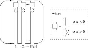
Figure 5.

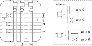
Figure 6. $K(m,n)$

We calculate $P_{0}(K(m,n))$. Using the relation of the HOMFLYPT polynomial, we obtain the relation

(4.3) $$P_{0}(K(m,n))=t^{2\varepsilon}P_{0}(K(m-\varepsilon,n))+\varepsilon t^{\varepsilon}P_{-1}(L(n)),$$

where $L(n)$ is illustrated in Figure 7, and $\varepsilon=1$ (resp. $-1$) if $m>0$ (resp. $m<0$). Since $Lk(L(n))=n$ and each component of $L(n)$ is trivial, it follows from (4.1) that

(4.4) $$P_{-1}(L(n);t)=t^{2n}(t^{-1}-t).$$

By combining (4.3) and (4.4),

$$P_{0}(K(m,n))=t^{2\varepsilon}P_{0}(K(m-\varepsilon,n))+\varepsilon t^{2n-1+\varepsilon}-\varepsilon t^{2n+1+\varepsilon}.$$

Since for each $\varepsilon(\in\{-1,1\}$)

$$\varepsilon t^{2n-1+\varepsilon}-\varepsilon t^{2n+1+\varepsilon}=t^{2n}-t^{2n+2\varepsilon},$$

we have

$$P_{0}(K(m,n))-t^{2n}=t^{2\varepsilon}(P_{0}(K(m-\varepsilon,n)-t^{2n}),$$

and hence

$$P_{0}(K(m,n))-t^{2n}=t^{2\varepsilon|m|}(P_{0}(K(0,n)-t^{2n})=t^{2m}(1-t^{2n}).$$

It follows that we have

$$P_{0}(K(m,n))=t^{2m}+t^{2n}-t^{2m+2n},$$

and so we have

(4.5) $$P_{0}^{(3)}(K(m,n))=-24mn(m+n-1).$$

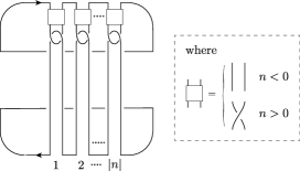
Figure 7. $L(n)$

By (4.2) and (4.5) we have the required formula

$$\overline{\mu}_{L}(I)\equiv-\frac{1}{3!2^{3}}\sum_{J<I}(-1)^{|J|}P_{0}^{(3)}(L_{J})-\frac{1}{2}x_{13}x_{24}(x_{13}+x_{24}-1)\pmod{\Delta_{L}(I)}.$$

References

- [1] T. Fleming, A. Yasuhara, Milnor’s invariants and self -equivalence, Proc. Amer. Math. Soc. 137 (2009), no. 2, 761–770.
- [2] K. Habiro, Claspers and finite type invariants of links, Geom. Topol. 4 (2000), 1–83.
- [3] T. Kanenobu, -moves and the HOMFLY polynomials of links, Bol. Soc. Mat. Mexicana (3) 10 (2004), 263–277.
- [4] T. Kanenobu, Y. Miyazawa, HOMFLY polynomials as Vassiliev link invariants, in Knot theory, Banach Center Publ. 42, Polish Acad. Sci., Warsaw (1998,) 165–185.
- [5] W. B. R. Lickorish, K. C.Millett, A polynomial invariant of oriented links, Topology 26 (1987), 107–141.
- [6] J.B. Meilhan, A. Yasuhara, Milnor invariants and the HOMFLYPT polynomial, Geom. Topol. 16 (2012), 889–917.
- [7] J. Milnor, Link groups, Ann. of Math. (2) 59 (1954), 177–195.
- [8] J. Milnor, Isotopy of links, Algebraic geometry and topology, A symposium in honor of S. Lefschetz, pp. 280–306, Princeton University Press, Princeton, N. J., 1957.
- [9] M. Polyak, On Milnor’s triple linking number, C. R. Acad. Sci. Paris Sé. I Math. 325 (1997), no. 1, 77–82.
- [10] A. Yasuhara, Self Delta-equivalence for Links Whose Milnor’s Isotopy Invariants Vanish, Trans. Amer. Math. Soc. 361 (2009), 4721–4749.