Geometrical scaling in high energy collisions
and its breaking

Abstract

We analyze geometrical scaling (GS) in Deep Inelstic Scattering at HERA and in pp collisions at the LHC energies and in NA61/SHINE experiment. We argue that GS is working up to relatively large Bjorken $x\sim 0.1$. This allows to study GS in negative pion multiplicity $p_{\rm T}$ distributions at NA61/SHINE energies where clear sign of scaling violations is seen with growing rapidity when one of the colliding partons has Bjorekn $x\geq 0.1$.

13.85.Ni,12.38.Lg

1 Introduction

In this short note, following Refs. [1]–[5] where also an extensive list of references can be found, we will focus on the scaling law, called geometrical scaling (GS), which has been introduced in the context of DIS [6]. Recently it has been shown that GS is also exhibited by the $p_{\text{T}}$ spectra at the LHC [1]–[3]. An onset of GS in heavy ion collisions at RHIC energies has been reported in Ref. [3]. At low Bjorken $x<x_{\mathrm{max}}$ proton is characterized by an intermediate energy scale $Q_{\text{s}}(x)$ – called saturation scale [7, 8] – defined as the border line between dense and dilute gluonic systems within a proton (for review see e.g. Refs. [9, 10]). For the present study, however, the details of saturation are not of primary interest, it is the very existence of $Q_{\text{s}}(x)$ which is of importance.

Here we present analysis of three different pieces of data which exhibit both emergence and violation of geometrical scaling. In Sect. 2 we briefly describe the method used to assess the existence of GS. Secondly, in Sect. 3 we describe our recent analysis [4] of combined HERA data [11] where it has been shown that GS in DIS works very well up to relatively large $x_{\text{max}}\sim 0.1$ (see also [12]). Next, in Sect. 4, on the example of the CMS $p_{\rm T}$ spectra in central rapidity [13], we show that GS can be extended to hadronic collisions. For particles produced at non-zero rapidities, one (larger) Bjorken $x=x_{1}$ may leave the domain of GS, i.e. $x_{1}>x_{\text{max}}$, and violation of GS should appear. In Sect. 5 we present analysis of very recent pp data from NA61/SHINE experiment at CERN [14] and show that GS is indeed violated once rapidity is increased. We conclude in Sect. 6.

2 Method of ratios

Geometrical scaling hypothesis means that some observable $\sigma$ that in principle depends on two independent kinematical variables, say $x$ and $Q^{2}$, in fact depends only on a specific combination of them denoted as $\tau$:

$$\sigma(x,Q^{2})=F(\tau)/{Q_{0}^{2}}.$$ (1)

Here function $F$ in Eq. (1) is a dimensionless function of scaling variable

$$\tau=Q^{2}/Q_{\text{s}}^{2}(x).$$ (2)

and

$$Q_{\text{s}}^{2}(x)=Q_{0}^{2}\left({x}/{x_{0}}\right)^{-\lambda}$$ (3)

is the saturation scale. Here $Q_{0}$ and $x_{0}$ are free parameters which can be extracted from the data within some specific model for $\sigma$, and exponent $\lambda$ is a dynamical quantity of the order of $\lambda\sim 0.3$. Throughout this paper we shall test the hypothesis whether different pieces of data can be described by formula (1) with constant $\lambda$, and what is the kinematical range where GS is working satisfactorily.

In view of Eq. (1) observables $\sigma(x_{i},Q^{2})$ for different $x_{i}$’s should fall on one universal curve, if evaluated not in terms of $Q^{2}$ but in terms of $\tau$. This means in turn that ratios

$$R_{x_{i},x_{\text{ref}}}(\lambda;\tau_{k})=\frac{\sigma(x_{i},\tau(x_{i},Q_{k}^{2};\lambda))}{\sigma(x_{\text{ref}},\tau(x_{\text{ref}},Q_{k,\text{ref}}^{2};\lambda))}$$ (4)

should be equal to unity independently of $\tau$. Here for some $x_{\rm ref}$ we pick up all $x_{i}<x_{\rm ref}$ which have at least two overlapping points in $Q^{2}$.

For $\lambda\neq 0$ points of the same $Q^{2}$ but different $x$’s correspond in general to different $\tau$’s. Therefore one has to interpolate $\sigma(x_{\text{ref}},\tau(x_{\text{ref}},Q^{2};\lambda))$ to $Q_{k,\text{ref}}^{2}$ such that $\tau(x_{\text{ref}},Q_{k,\text{ref}}^{2};\lambda)=\tau_{k}$. This procedure is described in detail in Refs. [4].

By tuning $\lambda$ one can make $R_{x_{i},x_{\text{ref}}}(\lambda;\tau_{k})\rightarrow 1$ for all $\tau_{k}$. In order to find optimal value $\lambda_{\rm min}$ that minimizes deviations of ratios (4) from unity we form the chi-square measure

$$\chi_{x_{i},x_{\text{ref}}}^{2}(\lambda)=\frac{1}{N_{x_{i},x_{\text{ref}}}-1}{\displaystyle\sum\limits_{k\in x_{i}}}\frac{\left(R_{x_{i},x_{\text{ref}}}(\lambda;\tau_{k})-1\right)^{2}}{\Delta R_{x_{i},x_{\text{ref}}}(\lambda;\tau_{k})^{2}}$$ (5)

where the sum over $k$ extends over all points of given $x_{i}$ that have overlap with $x_{\text{ref}}$, and ${N_{x_{i},x_{\text{ref}}}}$ is a number of such points.

3 Deep Inelastic Scattering at HERA

In the case of DIS the relevant scaling observable is $\gamma^{\ast}p$ cross section and variable $x$ is simply Bjorken $x$. In Fig. 1 we present 3-d plot of $\lambda_{\min}({x,x_{\rm ref}})$ which has been found by minimizing (5).

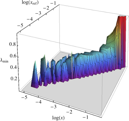
Figure 1: Three dimensional plot of $\lambda_{\mathrm{min}}(x,x_{\mathrm{ref}})$ obtained by minimization of Eq. (5).

Qualitatively, GS is given by the independence of $\lambda_{\text{min}}$ on Bjorken $x$ and by the requirement that the pertinent value of $\chi_{x,x_{\text{ref}}}^{2}(\lambda_{\text{min}})$ should be small (for the discussion of the latter see Refs. [4]). We see from Fig. 1 that the stability corner of $\lambda_{\text{min}}$ extends up to $x_{\text{ref}}\lesssim 0.1$, which is well above the original expectations. In Ref. [4] we have shown that:

$$\lambda=0.32-0.34\,\,\,\,\,{\rm for}\,\,\,\,\,x\leq 0.08.$$ (6)

4 Central rapidity $p_{\rm T}$ spectra at the LHC

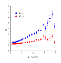
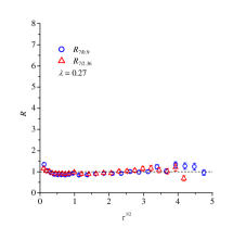
Figure 2: Ratios of CMS $p_{\mathrm{T}}$ spectra [13] at 7 TeV to 0.9 (blue circles) and 2.36 TeV (red triangles) plotted as functions of $p_{\mathrm{T}}$ (left) and scaling variable $\sqrt{\tau}$ (right) for $\lambda=0.27$.

In hadronic collisions at c.m. energy $W=\sqrt{s}$ particles are produced in the scattering process of two patrons carrying Bjorken $x$’s

$$x_{1,2}=e^{\pm y}\,p_{\text{T}}/W.$$ (7)

For central rapidities $x=x_{1}\sim x_{2}$. It has been shown that in this case charged particle multiplicity spectra exhibit GS [1]

$$\left.\frac{dN}{dyd^{2}p_{\text{T}}}\right|_{y\simeq 0}=\frac{1}{Q_{0}^{2}}F(\tau)$$ (8)

where $F$ is a universal dimensionless function of the scaling variable

$$\tau=p_{\text{T}}^{2}/Q_{\text{s}}^{2}(x)=p_{\text{T}}^{2}/Q_{0}^{2}\,\left(p_{\rm T}/(x_{0}\sqrt{s})\right)^{\lambda}.$$ (9)

Therfore the scaling observable is $\sigma(W,p_{\rm T}^{2})={dN}/{dyd^{2}p_{\text{T}}}$ and the method of ratios is applied to the multiplicity distributions at different energies ($W_{i}$ taking over the role of $x_{i}$ in Eq. (4)). For $W_{\rm ref}$ we take the highest LHC energy of 7 TeV. Therefore one can form two ratios $R_{W_{i},W_{\rm ref}}$ with $W_{1}=2.36$ and $W_{2}=0.9$ TeV. These ratios are plotted in Fig. 2 for the CMS single non-diffractive spectra for $\lambda=0$ and for $\lambda=0.27$, which minimizes (5) in this case. We see that original ratios plotted in terms of $p_{\text{T}}$ range from 1.5 to 7, whereas plotted in terms of $\sqrt{\tau}$ they are well concentrated around unity. The optimal exponent $\lambda$ is, however, smaller than in the case of DIS. Why this so, remains to be understood.

5 Violation of geometrical scaling in forward rapidity region

For $y>0$ two Bjorken $x$’s can be quite different: $x_{1}>x_{2}$. Therefore looking at the spectra with increasing $y$ one can eventually reach $x_{1}>x_{\mathrm{max}}$ and GS violation should be seen. To this end we shall use pp data from NA61/SHINE experiment at CERN [14] at different rapidities $y=0.1-3.5$ and at five different energies $W_{1,\ldots,5}=17.28,\;12.36,\;8.77,\;7.75$, and $6.28$ GeV.

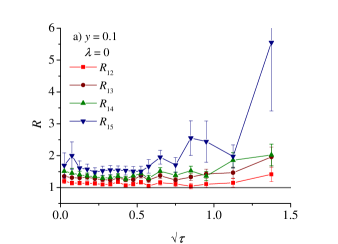
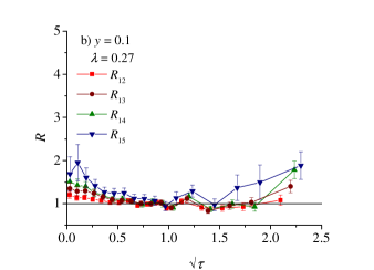
Figure 3: Ratios $R_{1k}$ as functions of $\sqrt{\tau}$ for the lowest rapidity $y=0.1$: a) for $\lambda=0$ when $\sqrt{\tau}=p_{\mathrm{T}}$ and b) for $\lambda=0.27$ which corresponds to GS.

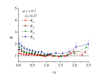
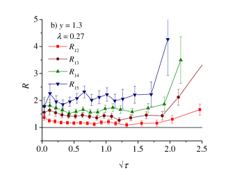
Figure 4: Ratios $R_{1k}$ as functions of $\sqrt{\tau}$ for $\lambda=0.27$ and for different rapidities a) $y=0.7$ and b) $y=1.3$. With increase of rapidity, gradual closure of the GS window can be seen.

In Fig. 3 we plot ratios $R_{1i}=R_{W_{1},W_{i}}$ (4) for $\pi^{-}$ spectra in central rapidity for $\lambda=0$ and 0.27. For $y=0.1$ the GS region extends towards the smallest energy because $x_{\rm max}$ is as large as 0.08. However, the quality of GS is the worst for the lowest energy $W_{5}$. By increasing $y$ some points fall outside the GS window because $x_{1}\geq x_{\rm max}$, and finally for $y\geq 1.7$ no GS should be present in NA61/SHINE data. This is illustrated nicely in Fig. 4.

6 Conclusions

We have shown that GS in DIS works well up to rather large Bjorken $x$’s with exponent $\lambda=0.32-0.34$. In pp collisions at the LHC energies in central rapidity GS is seen in the charged particle multiplicity spectra, however, $\lambda=0.27$ in this case. By changing rapidity one can force one of the Bjorken $x$’s of colliding patrons to exceed $x_{\rm max}$ and GS violation is expected. Such behavior is indeed observed in the NA61/SHINE pp data.

The author wants to thank M. Gazdzicki and Sz. Pulawski for the access to the NA61/SHINE data and to T. Stebel for collaboration and remarks. Many thanks are due to the organizers of this successful series of conferences. This work was supported by the Polish NCN grant 2011/01/B/ST2/00492.

References

- [1] L. McLerran and M. Praszalowicz, Acta Phys. Polon. B 41 (2010) 1917 and Acta Phys. Polon. B 42 (2011) 99.
- [2] M. Praszalowicz, Phys. Rev. Lett. 106 (2011) 142002.
- [3] M. Praszalowicz, Acta Phys. Polon. B 42 (2011) 1557 and arXiv:1205.4538 [hep-ph].
- [4] M. Praszalowicz and T. Stebel, JHEP 1303, 090 (2013) and arXiv:1302.4227 [hep-ph], to be published in JHEP.
- [5] M. Praszalowicz, arXiv:1301.4647 [hep-ph], to be published in Phys. Rev. D.
- [6] A. M. Stasto, K. J. Golec-Biernat and J. Kwiecinski, Phys. Rev. Lett. 86, 596 (2001).
-
[7]
L. V. Gribov, E. M. Levin and M. G. Ryskin, Phys. Rept. 100 (1983) 1;
A. H. Mueller and J-W. Qiu, Nucl. Phys. 268 (1986) 427; A. H. Mueller, Nucl. Phys. B558 (1999) 285. - [8] K. J. Golec-Biernat and M. Wüsthoff, Phys. Rev. D 59 (1998) 014017 and Phys. Rev. D 60 (1999) 114023.
- [9] A. H. Mueller, Parton Saturation: An Overview, arXiv:hep-ph/0111244.
- [10] L. McLerran, Acta Phys. Pol. B 41, 2799 (2010).
- [11] C. Adloff et al. [H1 Collaboration], Eur. Phys. J. C 21 (2001) 33; S. Chekanov et al. [ZEUS Collaboration], Eur. Phys. J. C 21 (2001) 443.
- [12] F. Caola, S. Forte and J. Rojo, Nucl. Phys. A 854, 32 (2011).
- [13] V. Khachatryan et al. [CMS Collaboration], JHEP 1002 (2010) 041 and Phys. Rev. Lett. 105 (2010) 022002 and JHEP 1101 (2011) 079.
-
[14]
N. Abgrall et al. [NA61/SHINE Collaboration],
Report from the NA61/SHINE experiment
at the CERN SPS CERN-SPSC-2012-029, SPSC-SR-107;
A. Aduszkiewicz, Ph.D. Thesis in prepartation, University of Warsaw, 2013;
Sz. Pulawski, talk at 9th Polish Workshop on Relativistic Heavy-Ion Collisions, Kraków, November 2012 and private communication.