Suppression of local heat flux in a turbulent magnetized intracluster medium

Abstract

X-ray observations of hot gas in galaxy clusters often show steeper temperature gradients across cold fronts – contact discontinuities, driven by the differential gas motions. These sharp (a few kpc wide) surface brightness/temperature discontinuities would be quickly smeared out by the electron thermal conduction in unmagnetized plasma, suggesting significant suppression of the heat flow across the discontinuities. In fact, the character of the gas flow near cold fronts is favorable for suppression of conduction by aligning magnetic field lines along the discontinuities. We argue that a similar mechanism is operating in the bulk of the gas. Generic 3D random isotropic and incompressible motions increase the temperature gradients (in some places) and at the same time suppress the local conduction by aligning the magnetic field lines perpendicular to the local temperature gradient. We show that the suppression of the effective conductivity in the bulk of the gas can be linked to the increase of the frozen magnetic field energy density. On average the rate of decay of the temperature fluctuations $\mathrm{d}\langle\delta T^{2}\rangle/\mathrm{d}t$ decreases as $\langle B^{2}\rangle^{-1/5}$.

1 Introduction

X-ray observations of galaxy clusters reveal significant spatial fluctuations of the gas temperature in a range of spatial scales (e.g. Markevitch et al., 2003). Given a temperature map with prominent fluctuations, it is possible to calculate an upper limit on the effective thermal conductivity, provided that the lifetime of the fluctuations can be estimated. It turns out to be at least an order of magnitude lower than the Spitzer conductivity for unmagnetized plasma (Ettori & Fabian, 2000; Markevitch et al., 2003).

Heat conduction in the intracluster medium (ICM) is primarily along the field lines because the Larmor radius of the particles is very small compared to the collisional mean free path (Braginskii, 1965). The ICM undergoes turbulent motion in a range of spatial scales (Inogamov & Sunyaev, 2003; Schuecker et al., 2004; Schekochihin & Cowley, 2006; Subramanian et al., 2006; Zhuravleva et al., 2011). As the magnetic field is, to a good approximation, frozen into the ICM, the field lines become tangled by gas motions and their topology changes constantly. Four main effects should be considered. First, parallel thermal conduction along stochastic magnetic field lines may be reduced because the heat-conducting electrons become trapped and detrapped between regions of strong magnetic field (magnetic mirrors; see Chandran & Cowley 1998; Chandran et al. 1999; Malyshkin & Kulsrud 2001; Albright et al. 2001). Secondly, diffusion in the transverse direction may be boosted due to spatial divergence of the field lines (Skilling et al., 1974; Rechester & Rosenbluth, 1978; Chandran & Cowley, 1998; Narayan & Medvedev, 2001; Chandran & Maron, 2004). Thirdly, there is effective diffusion due to temporal change in the magnetic field (‘field-line wandering’). Finally, if one is interested in temperature fluctuations and their diffusion, one must be mindful of the fact that the temporal evolution of the magnetic field is correlated with the evolution of the temperature field because the field lines and the temperature are advected by the same turbulent velocity field.

In this paper, we focus on the last effect. The more conventional approach, often used to estimate the relaxation of the temperature gradients, is to consider the temperature distribution as given and study the effect of a tangled magnetic field on the heat conduction. However, the direction and value of the fluctuating temperature gradients are not statistically independent of the direction of the magnetic-field lines because the latter are also correlated with the turbulent motions of the medium. We argue that, dynamically, the fluctuating gradients tend to be oriented perpendicular to the field lines and so heat fluxes are the more heavily suppressed the stronger the thermal gradients are. We also establish the relationship between the average conductivity and the growth of the magnetic energy density.

The structure of the paper is as follows. In Section 2, we provide a qualitative explanation of the correlation between the temperature gradients and the magnetic-field direction, accompanied by a number of numerical examples. In Section 3, a theoretical framework for modelling this effect is presented and the joint PDF of the thermal gradients, the angles between these gradients and the magnetic-field lines and the magnetic-field strength is derived in the solvable case of a simple model velocity field. The connection between the effective conductivity and the increase of the magnetic energy density is established. Analytical results are supplemented by numerical calculations in Section 3.4, which extrapolate our results to the case of a more general velocity field. In Section 4, we discuss the assumptions that have been necessary to enable analytical treatment, the consequent limitations on the applicability of our results, and also present some numerical tests using a global dynamical cluster simulation, which suggest that, at least qualitatively, our results survive when most of the simplifying assumptions are relaxed. Finally, in Section 5, we sum up our findings.

2 Qualitative discussion

We consider a volume of plasma with high electric conductivity and frozen-in magnetic field tangled on a scale much greater than the mean free path of the particles. We also assume the plasma motions to be incompressible, which is a good approximation for subsonic dynamics. Across the paper we treat the temperature as a passive scalar.

2.1 Illustrative example: conduction between converging layers of magnetised plasma

Consider two parallel layers of an incompressible medium vertically separated by distance $h$ with temperatures $T_{1}\neq T_{2}$. This is illustrated in Fig. 1: the direction of the field line is shown with the inclined solid line, making an angle $\theta$ with the vertical, so $\cos{\theta}=h/\sqrt{h^{2}+l^{2}}$, where $l$ is the horizontal distance between the footpoints of the field line anchored in the two layers. An incompressible flow with $\partial_{y}u_{y}<0$ reduces $h$ and increases $l$ so that $l\times h$ is conserved (in the absence of tangential shear). Here we are interested in the heat exchange between the layers, i.e. only the component of the heat flux along the temperature gradient $Q_{\nabla T}$ has to be calculated:

$$Q_{\nabla T}=\chi(\mn@boldsymbol{b}\cdot\nabla T)\cos{\theta}=\chi\frac{T_{2}-T_{1}}{\sqrt{h^{2}+l^{2}}}\frac{h}{\sqrt{h^{2}+l^{2}}}.$$ (1)

Let $h(t)=h_{0}f(t)$ and $l(t)=l_{0}/f(t)$. Then

$$Q_{\nabla T}=\chi\frac{T_{2}-T_{1}}{h_{0}}\frac{f}{\displaystyle f^{2}+(l_{0}/h_{0})^{2}f^{-2}},$$ (2)

where $\chi$ is the parallel thermal diffusivity coefficient (Braginskii, 1965), which is assumed constant across the volume for simplicity. Therefore, in the limit of $f\rightarrow 0$, $Q_{\nabla T}\rightarrow 0$ if $l_{0}\neq 0$. Similarly, when $f\rightarrow\infty$,  $Q_{\nabla T}\rightarrow 0$. The decrease of the heat flux at $f>1$ is simply due to the increase of the distance between the plates and corresponding decrease of the temperature gradient. The decrease at $f<1$ is due to systematic increase of the angle between the field lines and the direction of the temperature gradient.

If at some moment the field lines are tangled in such a way that all angles $\theta$ are equally probable, then parametrizing compression/stretching along $y$ by the same factor $f$ and averaging over $\theta$ gives us the suppressed heat flux along the temperature gradient:

$$Q_{\nabla T}=\chi\frac{T_{2}-T_{1}}{h_{0}}\frac{2f}{f^{2}+1}\\ (\mathrm{see~{}Fig.}~{}\ref{fig:func}).$$ (3)

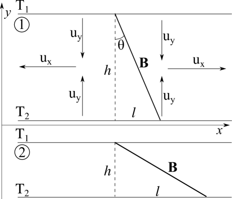
Figure 1: Correlated changes of the temperature gradients and the inclination of the magnetic-field lines in the case of a converging incompressible flow: plane parallel layers at different temperatures. Converging flow with $\partial_{y}u_{y}<0$ reduces $h$ and increases the temperature gradient $(T_{2}-T_{1})/h$, but suppresses heat flux. The solid line represents the direction of the magnetic field. If the medium is incompressible then $l\times h$ is conserved (in the absence of tangential shears).

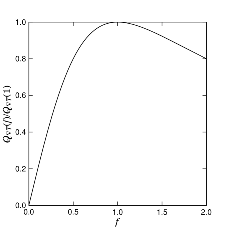
Figure 2: Suppression of the heat flux along the temperature gradient between two approaching/receding plates as a function of distance $f$ between the plates, when the medium between the plates is threaded by tangled magnetic field [see equation (3)]. At the initial moment ($f=1$), all angles between the magnetic field direction and the plates are equally probable. The decrease of the heat flux at $f>1$ is simply due to the increase of the distance between the plates and corresponding decrease of the temperature gradient. The decrease at $f<1$ is due to systematic increase of the angle between the field lines and the direction of the temperature gradient.

Thus, increasing the temperature gradient by squeezing the layers of the gas does not boost the heat exchange between them but rather makes it smaller. A qualitatively similar situation might occur at the cold fronts – contact discontinuities formed by differential gas motions, a very simple model of which is discussed in the next subsection.

2.2 Astrophysical example: model of a cold front

Chandra observations of galaxy clusters often show sharp discontinuities in the surface brightness of the ICM emission (see review by Markevitch & Vikhlinin, 2007). Most of these structures have lower-temperature gas on the brighter (higher-density) side of the discontinuity, suggesting that they are contact discontinuities rather than shocks. In the literature, these structures are called ‘cold fronts’. Because of the sharp temperature gradients, the limits on the thermal conduction derived for the observed cold fronts are strong (see e.g. Ettori & Fabian, 2000; Vikhlinin et al., 2001; Xiang et al., 2007).

In the majority of theoretical models, the formation of a cold front involves relative motion of cold and hot gases. Here we consider the case of a hot gas flowing around a colder, gravitationally bound gas cloud, which is a prototypical model of a cold front. For simplicity, we assume that the velocity field can be approximated with a 2D potential flow past a cylinder, while the initial temperature is symmetric around the cylinder. The initial temperature distribution and stream lines of the flow are shown in the left panel of Fig. 3. The middle panel shows the field lines of a random magnetic field superimposed on the initial temperature distribution. The evolved temperature and magnetic field are shown in the right panel of Fig. 3. Stretching of the fluid elements near the stagnation point along the front leads to the contraction of the same elements in the direction perpendicular to the front. This configuration has been considered in a number of studies of the cold fronts (see e.g. Asai et al., 2007; Churazov & Inogamov, 2004; Roediger et al., 2011; Lyutikov, 2006). Qualitatively, it corresponds to the situation sketched in Section 2.1 and Fig. 1, which naturally leads to the field lines orthogonal to the temperature gradient at the front.

Figure 3: Alignment of the field lines perpendicular to the temperature gradient for the velocity field characteristic of a cold front. A potential flow past a cylinder is used in this example. The left panel shows the initial temperature distribution (color image) and stream lines of the velocity field. The middle panel shows a random tangled magnetic field superposed on the initial temperature distribution. The right panel shows the time-evolved temperature map and magnetic-field lines (superposed contours) in such a flow. The flow boosts the temperature gradient at the cold front and at the same time stretches the field lines along the lines of constant temperature. In the resulting configuration, the field lines are essentially perpendicular to the sharp temperature gradient at the front.

2.3 Local correlation between the magnetic-field strength and the heat flux

Let us now discuss the suppression of the local heat flux in more general terms. Consider the induction equation for an incompressible medium and the advection equation for the temperature:

$$\frac{\mathrm{d}\mn@boldsymbol{B}}{\mathrm{d}t} = \mn@boldsymbol{B}\cdot\nabla\mn@boldsymbol{u},$$ (4)

$$\frac{\mathrm{d}T}{\mathrm{d}t} = 0,$$ (5)

where $\mn@boldsymbol{B}$ is the magnetic field, $\mn@boldsymbol{u}$ the velocity field, $T$ temperature and $\mathrm{d}/\mathrm{d}t=\partial/\partial t+\mn@boldsymbol{u}\cdot\nabla$. We have neglected thermal and magnetic diffusivities. While equation (5) is not a full magnetohydrodynamic energy equation, it is correct in the limit of an incompressible non-stratified medium (we will further discuss its applicability in Section 4). Let $\mn@boldsymbol{g}$ be the unit vector in the direction of the temperature gradient, $\mn@boldsymbol{b}$ the unit vector in the direction of the field line, $B$ the magnetic field magnitude and $G$ the temperature gradient magnitude, so $\mn@boldsymbol{B}=B\mn@boldsymbol{b}$, $\nabla T=G\mn@boldsymbol{g}$. The above equations imply

$$\frac{\mathrm{d}G}{\mathrm{d}t} = -G\mn@boldsymbol{g}\cdot(\nabla\mn@boldsymbol{u})\cdot\mn@boldsymbol{g},$$ (6)

$$\frac{\mathrm{d}B}{\mathrm{d}t} = B\mn@boldsymbol{b}\cdot(\nabla\mn@boldsymbol{u})\cdot\mn@boldsymbol{b},$$ (7)

$$\frac{\mathrm{d}\mu}{\mathrm{d}t} = \mu[\mn@boldsymbol{g}\cdot(\nabla\mn@boldsymbol{u})\cdot\mn@boldsymbol{g}-\mn@boldsymbol{b}\cdot(\nabla\mn@boldsymbol{u})\cdot\mn@boldsymbol{b}],$$ (8)

where $\mu=\mn@boldsymbol{b}\cdot\mn@boldsymbol{g}$, the cosine of the angle between $\mn@boldsymbol{B}$ and $\nabla T$. From these equations, we can immediately infer the following equation for $\mn@boldsymbol{b}\cdot\nabla T=G\mu$, a quantity proportional to the parallel heat flux:

$$\frac{\mathrm{d}\ln{(G\mu)}}{\mathrm{d}t}=-\frac{\mathrm{d}\ln{B}}{\mathrm{d}t}.$$ (9)

Thus, locally, the heat flux decreases as the field strength grows.

2.4 Numerical example: a random 2D velocity field

In this example, we consider a random temperature distribution and a random magnetic field in a random $\delta$-correlated-in-time (white) Gaussian 2D velocity field (Fig. 4). The temperature $T(x,y)$, the magnetic field $\mn@boldsymbol{B}(x,y)$ and the velocity field $\mn@boldsymbol{u}(x,y)$ (assumed incompressible, $\nabla\cdot\mn@boldsymbol{u}=0$) are modelled as superpositions of Fourier harmonics with random phases and amplitudes. The temperature and the magnetic field are advected according to equations (4) and (5). The velocity field is renewed at each time step (white-in-time field). The initial conditions are shown in the top panel of Fig. 4; there is no initial correlation between the temperature gradients and the orientation of the field lines. With time, preferential stretching/squeezing of the fluid elements leads to alignment of the field lines along the iso-temperature lines (see bottom panel in Fig. 4). This happens in all regions where the stretching/squeezing is sufficiently strong. As a result, the field lines are mostly perpendicular to the direction of the temperature gradient in all regions where the gradient is large. Intuitively, one expects that in a turbulent conducting medium, this tendency of local alignment between the magnetic filed and the isotherms will manifest itself statistically. In the next section, we work out a simple statistical model of this process.

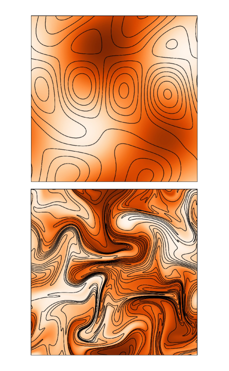
Figure 4: Alignment of the field lines perpendicular to the temperature gradient for a stochastic $\delta$-correlated-in-time Gaussian incompressible velocity field, modelled as a superposition of Fourier harmonics with random phases and amplitudes. The top panel shows the initial random temperature distribution (color) with the field lines of a random magnetic field superposed (they are uncorrelated with temperature). The bottom panel shows the same fields later on in the evolution. In the evolved image, field lines follow the lines of constant temperature in the regions where the temperature gradient is large.

3 Heat conduction in a stochastic velocity field

Here we treat the suppression of the heat conduction using an analytically solvable model that allows us to predict the statistical distribution of the cosine of the angle between the thermal gradient and the field line ($\mu$), the magnitude of the thermal gradient ($G$) and the magnetic-field strength ($B$). After the joint probability distribution function (PDF) of $\mu$, $G$ and $B$ is derived (Section 3.5), we will be in a position to assess how statistically prevalent the behaviour discussed in Section 2.4 is, but we will preface this detailed calculation with some simpler arguments to quantify the suppression of the heat flux.

3.1 Relaxation of temperature fluctuations

Let us restore heat conduction in equation (5):

$$\frac{\mathrm{d}T}{\mathrm{d}t}=\nabla\cdot(\chi\mn@boldsymbol{b}\mn@boldsymbol{b}\cdot\nabla T),$$ (10)

where $\chi$ is the parallel thermal diffusivity coefficient (Braginskii, 1965). Then the volume-averaged rate of change of the rms temperature fluctuations is

$$\frac{\mathrm{d}\langle\delta T^{2}\rangle}{\mathrm{d}t}=-2\chi\langle|\mn@boldsymbol{b}\cdot\nabla\delta T|^{2}\rangle=-2\chi\langle G^{2}\mu^{2}\rangle.$$ (11)

Thus, the average value of $G^{2}\mu^{2}$ characterizes the rate at which local temperature variations are wiped out by the thermal conduction.

3.2 Kazantsev-Kraichnan model

We consider the magnetic field to be so weak that it does not affect the velocity field. This condition is only satisfied if the magnetic energy density is much lower than the kinetic energy density of the plasma motions. This means that our model does not describe the saturated state, when these energy densities become comparable. The non-saturated regime could be a common transient situation in the ICM, at least locally, in the sense that at any given time, the magnetic field is amplified up to the saturation value only in a small fraction of the volume.

We will wish to calculate the joint PDF $p(\mu,G,B;t)$, where $\mu$ and $G$ are defined in Section 2, and investigate the evolution of the relevant correlations, viz., $\langle G^{2}\mu^{2}\rangle$ (see Section 3.1). To do that, we need to average the dynamical equations for $\mn@boldsymbol{g}$, $\mn@boldsymbol{b}$, $G$ and $B$ over all realizations of the stochastic velocity field. The equations are

$$\frac{\mathrm{d}g^{k}}{\mathrm{d}t} = -(\delta^{k}_{m}-g^{k}g^{m})g^{i}\partial_{m}u^{i},$$

$$\frac{\mathrm{d}b^{k}}{\mathrm{d}t} = (\delta^{k}_{i}-b^{k}b^{i})b^{m}\partial_{m}u^{i},$$

$$\frac{\mathrm{d}G}{\mathrm{d}t} = -Gg^{i}g^{m}\partial_{m}u^{i},$$

$$\frac{\mathrm{d}B}{\mathrm{d}t} = Bb^{i}b^{m}\partial_{m}u^{i},$$ (12)

where summation over repeated indices is implied.

This problem is solvable analytically for a Gaussian white-in-time velocity field (Kazantsev, 1968):

$$\langle u^{i}(t,\mn@boldsymbol{x})u^{j}(t^{\prime},\mn@boldsymbol{x}^{\prime})\rangle=\delta(t-t^{\prime})\kappa^{ij}(\mn@boldsymbol{x}-\mn@boldsymbol{x}^{\prime}),$$ (13)

where $\kappa^{ij}$ is the correlation tensor, whose form can be determined from symmetry and incompressibility considerations. We may assume the medium to be isotropic and homogeneous. Let us restrict our consideration to variation of magnetic field and temperature on spatial scales much smaller than that of the velocity field. Then, at any arbitrary point in space, the velocity can be expanded in linear approximation:

$$u^{i}(t,\mn@boldsymbol{x})=\sigma^{i}_{m}(t)x^{m},$$ (14)

where $\sigma^{i}_{m}(t)=\partial_{m}u^{i}$ and we have assumed $u^{i}(t,0)=0$ without loss of generality (otherwise change the reference frame). Then the velocity gradients satisfy

$$\left\langle\frac{\partial u^{i}}{\partial x^{m}}(t,\mn@boldsymbol{x})\frac{\partial u^{j}}{\partial x^{\prime n}}(t^{\prime},\mn@boldsymbol{x}^{\prime})\right\rangle\bigg{|}_{\mn@boldsymbol{x}=\mn@boldsymbol{x}^{\prime}} = \langle\sigma^{i}_{m}(t)\sigma^{j}_{n}(t^{\prime})\rangle$$ (15)

$$= \delta(t-t^{\prime})\kappa^{ij}_{mn},$$

where

$$\kappa^{ij}_{mn}=-\displaystyle\frac{\partial^{2}\kappa^{ij}(\mn@boldsymbol{y})}{\partial y_{m}\partial y_{n}}\bigg{|}_{\mn@boldsymbol{y}=0}\equiv\kappa T^{ij}_{mn}$$

and $\kappa=1/\tau_{eddy}$, $\tau_{eddy}$ being the turnover time of the turbulent eddies and

$$T^{ij}_{mn}=\delta^{ij}\delta_{mn}-\frac{1}{d+1}\left(\delta^{i}_{m}\delta^{j}_{n}+\delta^{i}_{n}\delta^{j}_{m}\right)$$ (16)

is the inevitable tensor form of $\kappa^{ij}_{mn}$ for an isotropic incompressible medium of dimension $d$ ($=2,~{}3$). This is the so-called Kazantsev-Kraichnan model, which has been a popular tool for modelling the properties of small-scale dynamo and passive-scalar advection in turbulent media (e.g., Chertkov et al., 1999; Balkovsky & Fouxon, 1999; Boldyrev & Schekochihin, 2000; Schekochihin et al., 2002, 2004; Boldyrev & Cattaneo, 2004, and references therein).

3.3 Relation between magnetic-field amplification and suppression of conduction for the white-in-time velocity field

Before presenting the full statistical calculation, we wish to give a relatively simple one that establishes the connection between the relaxation rate of the temperature fluctuations and the magnetic-energy density. The heat flux along the field line $G\mu$ is inversely proportional to the length of a field-line segment $s$. Therefore, one can relate the change of the mean square heat flux $\langle G^{2}\mu^{2}\rangle$, which is also the decay rate of the temperature fluctuations (see Section 3.1), to the growth of the magnetic-energy density as follows:

$$\langle B^{2}\rangle\propto\langle s^{2}\rangle,~{}\langle G^{2}\mu^{2}\rangle\propto\langle 1/s^{2}\rangle.$$ (17)

As explained in Section 3.2, we assume an isotropic linear random velocity field. Let it be piecewise constant in time over intervals $\tau_{c}$ and completely uncorrelated for $\Delta t>\tau_{c}$. Assume further that the amount of stretching of any fluid element over individual time intervals of duration $\sim\tau_{c}$ is small compared to the size of the element, which amounts to a model of white-noise field. Under these assumptions, it is easy to obtain the PDF of $s$ as a function of time $t$ in the limit $t/\tau_{c}\gg 1$. The evolution of each component of the separation vector $\mn@boldsymbol{x}$ of any two locations frozen into a velocity field constant over time interval $\tau_{c}$ is

$$x^{i}(\tau_{c})\approx x^{i}(0)+\tau_{c}\sigma^{i}_{j}x^{j}(0)+\frac{1}{2}\tau_{c}^{2}\sigma^{i}_{j}\sigma^{j}_{k}x^{k}(0)+O(\tau_{c}^{3}),$$ (18)

where $\sigma^{i}_{j}$ is the velocity gradients matrix [see equation (14)]. Since we are dealing with a random isotropic field, we can set $\mn@boldsymbol{x}(0)=(1,0,0)$ at $t=0$. Then

$$x^{1}(\tau_{c})\approx 1+\tau_{c}\sigma^{1}_{1}+\frac{1}{2}\tau_{c}^{2}\sigma^{1}_{j}\sigma^{j}_{1}+O(\tau_{c}^{3}),$$

$$x^{i\neq 1}(\tau_{c})=\tau_{c}\sigma^{i}_{1}+O(\tau_{c}^{2}).$$ (19)

We are interested in the time evolution of the ‘stretching factor’ $s^{2}=|\mn@boldsymbol{x}|^{2}$. For one ‘act of stretching’, equation (19) implies

$$\ln{s^{2}(\tau_{c})}=2\tau_{c}\sigma^{1}_{1}-2\tau_{c}^{2}(\sigma^{1}_{1})^{2}+\tau_{c}^{2}\sigma^{j}_{1}\sigma^{j}_{1}+\tau_{c}^{2}\sigma^{1}_{j}\sigma^{j}_{1}+O(\tau_{c}^{3}).$$ (20)

For $t\gg\tau_{c}$, the calculation of $s^{2}(t)$ reduces to summation of $N=t/\tau_{c}\gg 1$ such independent stretching episodes:

$$\ln{s^{2}(t)}=\sum{\ln{s^{2}(\tau_{c})}}.$$ (21)

After applying the central limit theorem to $(1/N)\sum\ln{s^{2}(\tau_{c})}$, one readily gets the PDF of $s^{2}$:

$$P(s^{2})=\frac{1}{s^{2}}\frac{1}{\sqrt{2\pi\sigma^{2}_{s}}}\exp\left[-\frac{\left(\ln{s^{2}}-m_{s}\right)^{2}}{2\sigma^{2}_{s}}\right],$$ (22)

where

$$\sigma_{s} = 2\sqrt{T_{11}^{11}\frac{t}{\tau_{eddy}}},$$

$$m_{s} = \left[-2T_{11}^{11}+\sum_{i=1}^{d}\left(T_{11}^{ii}+T_{1i}^{i1}\right)\right]\frac{t}{\tau_{eddy}},$$ (23)

where $\tau_{eddy}$ and $T^{ij}_{mn}$ are defined at the end of Section 3.2. We have taken $\delta(0)=1/\tau_{c}$ in equation (15). Using equation (17), we get

$$\langle B^{2}\rangle\propto e^{m_{s}+\sigma_{s}^{2}/2},~{}\langle G^{2}\mu^{2}\rangle\propto e^{-m_{s}+\sigma_{s}^{2}/2}.$$ (24)

This leads to a simple relation between the growing magnetic-energy density and the evolution of the mean square heat flux:

$$\langle G^{2}\mu^{2}\rangle\propto\langle B^{2}\rangle^{p},~{}\mathrm{where}~{}p=\frac{-m_{s}+\sigma_{s}^{2}/2}{~{}~{}m_{s}+\sigma_{s}^{2}/2}.$$ (25)

For an incompressible velocity field in 3D, using equation  (16), we get $p=-1/5$. This is a statistical version of the dynamical equation (9). It implies that on average, as the magnetic-energy density grows, the rate of decay of the temperature fluctuations is reduced, although the efficiency of this reduction is modest ($p$ is low). This is because $\langle G^{2}\mu^{2}\rangle$ is dominated by regions of low stretching while $\langle B^{2}\rangle$ by regions of high stretching [equation (17)] and the distribution of these is highly intermittent.

3.4 Finite-time-correlated velocity field

How sensitive is this result to the obviously unphysical assumption of zero correlation time? Here, we numerically calculate the PDF of $s$ in a random incompressible 3D velocity field evolving according to a Langevin equation with a finite correlation time. This is a generalization of the $\delta$-correlated case considered in Section 3.3.

We consider a large number of independent field-line segments, each one placed in its own stochastic incompressible velocity field, given by equation (14), with the velocity gradient satisfying

$$\frac{\mathrm{d}\sigma^{i}_{m}}{\mathrm{d}t}=-\frac{1}{\tau_{c}}\sigma^{i}_{m}+\partial_{m}a^{i},$$ (26)

where $\tau_{c}$ is the correlation time and $a^{i}$ is a stochastic Gaussian acceleration whose gradient satisfies

$$\langle\partial_{m}a^{i}(t)\partial_{n}a^{j}(t^{\prime})\rangle=\delta(t-t^{\prime})A^{2}T^{ij}_{mn}.$$ (27)

Here $A^{2}$ is the noise amplitude and the dimensionless tensor $T^{ij}_{mn}$ is fixed by isotropy and incompressibility as given by equation (16). It is possible to define the effective turn-over time of turbulent eddies $\tau_{eddy}$ in much the same way as we we did for the $\delta$-correlated case:

$$\int_{0}^{\infty}\langle\sigma^{i}_{m}(0)\sigma^{j}_{n}(t)\rangle\mathrm{d}t=\frac{1}{2}A^{2}\tau_{c}^{2}T^{ij}_{mn}\equiv\frac{1}{2\tau_{eddy}},$$ (28)

where the exact solution of the Langevin equation (26) has been substituted. Thus, $\tau_{eddy}=1/(\tau_{c}A)^{2}$.

In view of equation (17), the evolution of $\langle G^{2}\mu^{2}\rangle$ and $\langle B^{2}\rangle$ can be easily calculated from the distribution of the segment lengths. Here we do this for a range of values of the ratio $\tau_{c}/\tau_{eddy}$. In Section 3.3, we treated the case $\tau_{c}/\tau_{eddy}\rightarrow 0$ analytically, whereas for a physically sound case, $\tau_{c}/\tau_{eddy}\approx 1$ because typically turbulent velocities decorrelate over their eddy turnover times and fluid elements are stretched by order-unity amounts over the same time scales. The results are shown in Fig. 5. Even though the growth/decay rates of $\langle B^{2}\rangle$ and $\langle G^{2}\mu^{2}\rangle$ do change with correlation time, their relative behaviour appears to be invariant, viz.,

$$\langle G^{2}\mu^{2}\rangle\propto\langle B^{2}\rangle^{-1/5},$$ (29)

practically the same as for the $\delta$-correlated regime [cf. equation (25)]

Thus, finite correlation times do not change the form of the effective conduction-magnetic-energy-density relation, only modifying the time dependence. This result gives us some confidence in the Kazantsev-Kraichan velocity as a credible modelling choice.

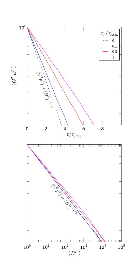
Figure 5: The decrease of the mean square heat flux $\langle G^{2}\mu^{2}\rangle$ for the time-correlated velocity field and different ratios $\tau_{c}/\tau_{eddy}$ (numerical results). While growth/decay rates of $\langle B^{2}\rangle$ and $\langle G^{2}\mu^{2}\rangle$ change with correlation time, their relative behavior is practically the same: $\langle G^{2}\mu^{2}\rangle\propto\langle B^{2}\rangle^{-0.2}$.

3.5 Statistics of the heat flux

In this section we will finally derive the full joint statistical distribution of the fluctuating magnetic fields and temperature gradients and hence the detailed correlations between the heat flux, the field strength and the relative direction of the magnetic field and the temperature gradient.

For a velocity field given by equation (14), we can write equations (12) for $\mn@boldsymbol{g}$, $\mn@boldsymbol{b}$, $G$ and $B$ as follows:

$$\partial_{t}g^{k} = -(\delta^{k}_{m}-g^{k}g^{m})g^{i}\sigma^{i}_{m},$$

$$\partial_{t}b^{k} = (\delta^{k}_{i}-b^{k}b^{i})b^{m}\sigma^{i}_{m},$$

$$\partial_{t}G = -Gg^{i}g^{m}\sigma^{i}_{m},$$

$$\partial_{t}B = Bb^{i}b^{m}\sigma^{i}_{m}.$$ (30)

There are no advection terms here due to the homogeneity of the gas [so we can consider equation (12) at $\mn@boldsymbol{x}=0$].

The details of the derivation of the equation for the joint PDF $p(\mu,G,B;t)$ are presented in Appendix A. The result is

$$\partial_{t}p=\frac{\kappa}{2(d+1)}[2d(1-\mu^{2})(\mu\partial_{\mu}\mu\partial_{\mu}-\partial_{G}G\mu\partial_{\mu}-\partial_{B}B\mu\partial_{\mu})$$ (31)

$$+(d-1)(\partial_{G}G\partial_{G}G+\partial_{B}B\partial_{B}B)+2(1-\mu^{2}d)\partial_{G}G\partial_{B}B$$

$$+d(d+1-2d\mu^{2})(2\mu\partial_{\mu}-\partial_{G}G-\partial_{B}B)$$

$$+2d^{2}(1-d\mu^{2})]p,$$

where $d$ is the dimension of space. From now on, we only consider $d=3$.

Multiplying both sides of equation (31) by $G^{2}\mu^{2}$ and integrating, we find

$$\partial_{t}\langle G^{2}\mu^{2}\rangle=-\frac{{\kappa}}{2}\langle G^{2}\mu^{2}\rangle,$$ (32)

so the mean square heat flux decays exponentially in time. Then, recalling equation (11) for the rate of smoothing of the temperature fluctuations,

$$\frac{\mathrm{d}\langle\delta T^{2}\rangle}{\mathrm{d}t}\propto-e^{-\kappa t/2}\rightarrow 0.$$ (33)

We observe that the relaxation rate of the temperature fluctuations decreases significantly on time-scales of the order of the turnover time of the turbulent eddies ($\kappa=1/\tau_{eddy}$).

It is also possible to recover the relation for the mean square heat flux as a function of the magnetic-energy density [equation (25)]. Multiplying equation (31) by $B^{2}$ and integrating, we obtain the evolution of the magnetic energy density:

$$\partial_{t}\langle B^{2}\rangle=\frac{5}{2}\kappa\langle B^{2}\rangle.$$ (34)

This result, combined with equation (32), leads to the relation established in Section 3.3:

$$\langle G^{2}\mu^{2}\rangle=\langle B^{2}\rangle^{-1/5}.$$ (35)

We expect that the temperature gradients and the magnetic-field lines will become perpendicular to each other. Let us then first investigate the limit of $\mu\rightarrow 0$, in which equation (31) can be solved analytically. Let $x=\ln{\mu}$, $y=\ln{G}$ and $z=\ln{B}$. Then the joint PDF of these variables is $h(x,y,z;t)=p(\mu(x),G(y),B(z);t)e^{x+y+z}$, where the last factor is the Jacobian of the transformation of variables. Taking $\mu\rightarrow 0$ in equation (31), we find that $h$ satisfies

$$\partial_{t}h=\frac{\kappa}{4}[3h_{xx}+h_{yy}+h_{zz}-3(h_{xy}+h_{xz})+h_{yz}$$ (36)

$$+3(2h_{x}-h_{y}-h_{z})].$$

Let us now write $h$ in the following form:

$$h(x,y,z;t)=f(x,y;t)\delta(x+y+z).$$ (37)

Substituting this ansatz into equation (36), we find that the factorization goes through and $f$ satisfies

$$\partial_{t}f=\frac{\kappa}{4}[3f_{xx}+f_{yy}-3f_{xy}+3(2f_{x}-f_{y})].$$ (38)

This factorization implies that in the limit $\mu\rightarrow 0$, $G\mu\propto 1/B$ independently of the initial conditions. This result was anticipated in Section 3.3, where we took the ratio of $G\mu$ and $1/B$ to be the same for all the segments of the field lines at the initial moment.

Let us make another transformation: $\xi=x=\ln{\mu}$ and $\eta=x+2y=\ln{(G^{2}\mu)}$ to separate variables in equation (38). The joint PDF of these two variables, $w(\xi,\eta;t)=f(x(\xi),y(\xi,\eta);t)$, satisfies

$$\partial_{t}w=\frac{\kappa}{4}(3w_{\xi\xi}+w_{\eta\eta}+6w_{\xi}).$$ (39)

This equation can be readily solved:

$$w(\xi,\eta;t)=\frac{1}{\sqrt{3}\pi\kappa t}\int_{-\infty}^{+\infty}\mathrm{d}\xi^{\prime}\mathrm{d}\eta^{\prime}w(\xi^{\prime},\eta^{\prime};0)e^{-\frac{1}{3\kappa t}\left[\frac{3}{2}\kappa t+(\xi-\xi^{\prime})\right]^{2}}$$ (40)

$$\times e^{-\frac{1}{\kappa t}(\eta-\eta^{\prime})^{2}}.$$

Notice that along with diffusion in both variables, the PDF drifts to $\xi\rightarrow-\infty$, i.e to smaller $\mu$. So there is a continued tendency towards mutually perpendicular orientation of the thermal gradients and the field lines.

If one is interested how the joint PDF of $\mu$ and $G$ behaves in the case of $\mu$ of order unity, the full equation (31) integrated over $B$ has to be solved. Technically speaking, we are obliged to do this in order to ascertain that the limit $\mu\rightarrow 0$ was the relevant one to consider, i.e. that the joint distribution of $\mu$ and $G$ moves towards smaller $\mu$ independently of initial conditions. Again, to separate variables, we employ the variables $\xi=\ln{\mu}$ and $\eta=\ln{(G^{2}\mu)}$. The PDF of these variables, $w(\xi,\eta;t)=\int p(\mu(\xi),G(\xi,\mu),B;t)e^{\frac{1}{2}(\xi+\eta)}\mathrm{d}B$, satisfies

$$\partial_{t}w=\frac{{\kappa}}{4}[3(1-e^{2\xi})w_{\xi\xi}+(1+3e^{2\xi})w_{\eta\eta}$$ (41)

$$+6(1-2e^{2\xi})w_{\xi}-12e^{2\xi}w].$$

In order to solve this equation numerically, it is convenient to rewrite it in the divergence form as follows:

$$\partial_{t}w=\frac{{\kappa}}{4}\{\partial_{\xi}[2(1-e^{2\xi})+(1-e^{2\xi})\partial_{\xi}]$$ (42)

$$+\partial_{\eta}(1+3e^{2\xi})\partial_{\eta}\}w.$$

Numerical solution of this equation is presented in Fig. 6. With time, the maximum of the PDF does indeed shift towards smaller $\mu$, demonstrating that the temperature gradient and the magnetic-field vector are becoming ever more orthogonal to each other. One can replot this graph in coordinates $G\mu$ (heat flux) and $G$ to observe that the rate of smearing of the temperature fluctuations in equation (11) is correlated with the magnitude of the temperature gradients (Fig. 7) in such a way that sharper gradients on average tend to be wiped out slower due to smaller corresponding values of $G\mu$.

Figure 6: Evolution of the joint PDF of $\mu$ and $G$ at regular time intervals from $t=0$ to $t=\tau_{eddy}$ (turn-over time of the turbulent eddies) obtained via numerical solution of the equation (42). The maximum of the function drifts to the region where the thermal gradients and the field lines are perpendicular ($\mu\rightarrow 0$).

Figure 7: Evolution of the joint PDF in terms of heat flux $G\mu=|\mn@boldsymbol{b}\cdot\nabla T|$ and $G=|\nabla T|$ at the same times as in Fig. 6. Sharper gradients tend to be wiped out slower due to the smaller corresponding values of the heat flux.

4 Limitations of our theory and a numerical test

We now discuss the assumptions we have made in our theory and the extent to which they limit its applicability.

4.1 Spatial scales

The ordering of scales in the problem considered in this paper obeys the following relations:

$$\rho_{e}\ll\lambda_{mfp}\lesssim l\lesssim\lambda_{u},$$ (43)

where $l$ is the characteristic size of the region we deal with, $\rho_{e}$ is the electron Larmor radius, $\lambda_{mfp}$ is the electron mean-free path and $\lambda_{u}$ is the typical size of a turbulent eddy.

The limit $l\ll\lambda_{u}$ simplifies the calculation of the field-line stretching because the linear expansion of the velocity field can be used [equation (14)]. This allows for an analytic treatment of the problem. Note that the kinematic dynamo naturally sets the parallel correlation length of the magnetic field $\lambda_{B\parallel}$ to be $\sim\lambda_{u}$ (Schekochihin et al., 2002, 2004).

The condition $\lambda_{mpf}\lesssim l$ allows us to apply the thermal conduction equation (10) at these spatial scales. Due to the fact that in the kinematic-dynamo regime, $\lambda_{u}\sim\lambda_{B\parallel}$, we also have $\lambda_{mfp}\lesssim\lambda_{B\parallel}$. This limit being assumed, we can ignore the magnetic mirroring effects because the electrons are free to escape magnetic traps via collisional pitch-angle scattering (Chandran & Cowley, 1998; Chandran et al., 1999).

The typical value of the mean-free path between Coulomb collisions,

$$\lambda_{mfp}\sim 8~{}{\rm kpc}\left(\frac{T}{5~{}{\rm KeV}}\right)^{2}\left(\frac{n_{e}}{10^{-3}~{}{\rm cm^{-3}}}\right)^{-1},$$ (44)

varies in cluster cores from $0.01$ to $20$ kpc depending on their temperature and density. For example, in the core of the Coma cluster, the mean-free path is $\sim 5$ kpc (Churazov et al., 2012); in M87/Virgo, it is much smaller, $\lambda_{mfp}\sim 0.01$ kpc, due to lower temperature and higher density (Churazov et al., 2008). On the other hand, the value of $\lambda_{u}$ can be in the range of 10 kpc to 200 kpc (Inogamov & Sunyaev, 2003; Schuecker et al., 2004; Schekochihin & Cowley, 2006; Subramanian et al., 2006; Zhuravleva et al., 2011; Kunz et al., 2011). Therefore, our analysis is relevant for temperature fluctuations on scales in the range $10^{-1}\mbox{--}10^{2}$ kpc. Some of these scales are directly resolvable with Chandra or XMM-Newton, suggesting that in observed substructures in the temperature maps, the isotemperature contours should be roughly aligned with the magnetic-field lines.

4.2 Incompressibility

The assumption of incompressibility [needed to use equation (16] for the description of the velocity field) is valid as long as the gas velocities are subsonic. This is reasonable for the ICM, except for cases of strong mergers or AGN-driven strong shocks in the very core of a cluster. The comparison of cluster-mass estimates from X-ray data and lensing or stellar kinematics (e.g. Churazov et al., 2008) and simulations (e.g. Lau et al., 2009) suggest that the kinetic energy of the gas motions is at the level of 5-15% of its thermal energy in relaxed clusters. Slight deviations from incompressibility should not dramatically alter our results.

4.3 Stratification

We have neglected the effects of stratification. It is well known that in the ICM anisotropic thermal conduction modifies the classical Schwarzschild stability criterion in such a way that any radial temperature gradient leads to an instability: the magnetothermal instability (MTI, Balbus 2000) if the thermal gradient and the gravity force are codirectional and the heat-flux-driven buoyancy instability (HBI, Quataert 2008) if they are oppositely directed. These instabilities have been extensively studied in numerical simulations (Sharma et al., 2009; Parrish et al., 2009; Bogdanović et al., 2009; Ruszkowski & Oh, 2010; Ruszkowski et al., 2011; McCourt et al., 2011; Kunz et al., 2012).

However, the instabilities are driven by large-scale mean gradients and in a turbulent plasma, at small enough scales, the buoyancy effects are likely to be less important than turbulent motions (cf. Ruszkowski & Oh, 2010) — essentially because turbulent time-scales get shorter at shorter spatial scales, while the buoyancy timescale is fixed. Indeed, the typical turbulent timescale is $\tau_{turb}\sim\lambda_{u}/u=\lambda_{u}/(Mc_{s})$, where $u$ is the (subsonic) velocity of turbulent motion, $M$ is the Mach number, $c_{s}$ is the speed of sound; in contrast, the buoyancy time-scale is $\tau_{buoy}\sim\sqrt{l_{P,T}/g}\sim\sqrt{l_{P,T}l_{P}}/c_{s}$, where $g$ is the gravitational acceleration caused by the cluster potential, $l_{P}$ is the characteristic length of change of the pressure profile and $l_{T}$ (in the case of MTI/HBI) is that of the macroscopic temperature profile. Therefore, $\tau_{turb}\lesssim\tau_{buoy}$ if $\lambda_{u}\lesssim Ml_{P}$ or $\lambda_{u}\lesssim M\sqrt{l_{P}l_{T}}$ (for MTI/HBI). Let $M$ be $\sim 0.3$. For typical cluster core parameters ($l_{P}\sim 100$ kpc, $l_{T}\sim 300$ kpc), we get $\lambda_{u}\lesssim 50$ kpc; for the bulk ($l_{P}\sim 300$ kpc, $l_{T}\sim 1000$ kpc), we get $\lambda_{u}\lesssim 200$ kpc.

Thus, our results apply at smaller spatial scales, where the turbulence time-scales are shorter than the buoyancy time-scale. Obviously, one cannot neglect stratification while constructing a full self-consistent model of the ICM, but comparison with global cluster simulations (Section 4.7) suggests that accounting for buoyancy does not eliminate the phenomenon of local orthogonalization of the field lines and temperature gradients.

4.4 Thermal conduction

Our model requires the eddy turnover time to be smaller than the conduction time, which is quite a serious restriction. Applying the standard formula for the Spitzer thermal conduction timescale, one gets

$$\tau_{cond}\sim n_{e}k_{B}l^{2}/\kappa_{Sp}\approx 3\times 10^{7}\left(\frac{n_{e}}{10^{-3}{\rm cm}^{-3}}\right)\left(\frac{l}{100~{}{\rm kpc}}\right)^{2}$$ (45)

$$\times\left(\frac{T_{e}}{5~{}{\rm KeV}}\right)^{-5/2}~{}{\rm yr},$$

where $n_{e}$ is the electron density, $T_{e}$ the electron temperature and $\kappa_{Sp}$ the Spitzer thermal conductivity. At the same time,

$$\tau_{turb}\sim 5\times 10^{8}~{}\left(\frac{\lambda_{u}}{100~{}{\rm kpc}}\right)\left(\frac{M}{0.3}\right)^{-1}~{}{\rm yr}.$$ (46)

From this estimate, it is clear that in the cool cores, the conduction time-scale can be longer than that of the turbulence, but in the hot ($\sim 8~{}{\rm KeV}$) and rarefied ICM outside the core, the conduction time-scale can instead be much shorter.

Nevertheless, even outside the core the orthogonalization of the temperature gradients and field lines is likely to take place. Qualitatively, this is because the effect of the orthogonalization is to switch off conduction, i.e. effectively lengthen the conduction time-scale compared to the estimate (45). Thus, while gradients codirectional with field lines at some initial moment may be quickly erased by conduction, the ones that make large angles with the field lines can survive longer and, as turbulence orthogonalizes them further, conduction will become increasingly inefficient. In other words, the assumption of slow conduction will become better satisfied as the evolution proceeds. We will see that these qualitative arguments are indeed corroborated by cluster simulations with anisotropic conduction (§ 4.7).

4.5 Dynamics of the magnetic field

As shown in Section 3.3, the evolution of the decay rate of the small-scale ($l\lesssim\lambda_{u}$) temperature variations can be linked to the amount of stretching of the field lines as $\propto\langle 1/s^{2}\rangle$. Essentially the decay rate goes down because the field lines, along which the heat is transported, are stretched. The amount of stretching is, of course, limited by saturation of the magnetic field. This may turn out to be a key effect in the problem, but it is not analytically treatable as easily as the case of passive field considered here and is best addressed with direct numerical simulations (see Section 4.7). Another potentially important effect we have ignored is the reconnection of the field lines, which may in principle considerably modify their topology. While we believe the simple model considered in this paper correctly captures the qualitative picture, direct numerical simulations are required to confirm this.

4.6 Local versus global conduction

We stress again that we have only considered the suppression of local thermal conduction, as applies to temperature fluctuations on scales $l<\lambda_{u}$. We have established that the gradients associated with these fluctuations are predominantly oriented perpendicular to the magnetic-field lines by the plasma flow. In general, however, if one is interested in the global heat transport on scales $l\gg\lambda_{u}$, other effects start to be important: in particular, exponential divergence of field lines (Rechester & Rosenbluth, 1978; Narayan & Medvedev, 2001; Chandran & Maron, 2004).

4.7 Comparison with global cluster simulations

To back up our qualitative arguments in support of the conclusions of our theoretical model despite the many simplifying assumptions that were required to make it solvable, we have employed the data drawn from the simulations reported by ZuHone et al. (2013). These are global dynamic MHD simulations of a disturbed cluster, which were not specifically designed to test our model but represent a current state-of-the-art numerical model of cluster evolution in response to a minor merger. The simulations incorporate all of the additional physics that we neglected and that is essential for a global model: a range of spatial and time-scales, compressibility, large-scale stratification, buoyancy, anisotropic thermal conduction, radiative cooling and dynamic back-reaction of the magnetic field on the fluid motions.

Figure 8: Central 500-kpc region of the simulation box of ZuHone et al. (2013) at $t=5.5~{}{\rm Gyr}$ used for comparison of our theory with the simulations.

In these simulations, a massive ($M\approx 1.5\times 10^{15}~{}M_{\odot}$, $T\sim 8$ keV), cool-core cluster, initially in hydrostatic equilibrium, merged with a small (mass ratio $R=5$) gasless subcluster, which set off the sloshing of the cool core. The simulation started at a point in time when the cluster centers had a mutual separation of $d=3$ Mpc and an impact parameter $b=500$ kpc. The initial velocities of the subclusters were set up assuming that the total kinetic energy of the system was set to half of its total potential energy. The main cluster was set up within a cubical computational domain of width $L=2.4$ Mpc on a side, with the finest cell size on the grid of 2.34 kpc. A random magnetic field was set up in Fourier space using independent normal random deviates for the real and imaginary components of the field. The field spectrum corresponded to a Kolmogorov shape with cut-offs at large ($\approx 500$ kpc) and small ($\approx 40$ kpc) linear scales. The initial plasma $\beta$ was 400. For the detailed description of these simulations, see ZuHone et al. (2013) and ZuHone et al. (2011). In the tests reported below, we only considered the central 500 kpc of the simulated cluster (Fig. 8), where the disturbance of the ICM was greatest, leading to significant local temperature variation and tangled magnetic field.

First, we examined a simulation with thermal conduction and radiative cooling turned off – this is the Run S1 from ZuHone et al. (2013). Fig. 9 shows the evolution of the joint PDF$(G,\mu)$ analogous to that shown in Fig. 6. Initially, the magnetic field orientation was random as indicated by the flat PDF over $\mu$ in the top left frame in Fig. 9. With time, the most probable value of $G$ increased, while the corresponding $\mu$ decreased. This behavior is qualitatively very similar to the evolution of the model PDF shown in Fig. 6. Note that in Fig. 8, it is visually manifest that magnetic field lines and surfaces of constant temperature are aligned in much of the disturbed ICM, including both sharp fronts (cf. Section 2.2) and the more random turbulent regions.

When radiative cooling was switched on, while conduction was still off (Run SX of ZuHone et al. 2013), the behaviour of the joint PDF of $G$ and $\mu$ was qualitatively very similar to that in pure MHD case described above, except for a small increase of the PDF at higher gradients independent of the value of $\mu$, which is expected because cooling may generate temperature gradients from the density gradients regardless of the magnetic-field orientation.

Finally, consider a simulation identical to the ones used above but with both cooling and anisotropic conduction switched on (Run SCX1 of ZuHone et al. 2013). In Fig.  10, the joint PDF of $G$ and $\mu$ for the cluster, taken at a late stage in its evolution, is contrasted to the case without conduction at a similar time. For this hot ($T\sim 8~{}{\rm KeV}$) simulated cluster, thermal conduction was strong enough to make a non-trivial impact on the PDF. Efficient anisotropic conduction quickly eliminated small-scale thermal gradients in the regions where the field lines and the temperature gradients were aligned in the initial setup, while the gradients orthogonal to the field survived longer. This process shifted the PDF to smaller $\mu$ and lower $G$ as compared to the case with no conduction (see Fig. 9). At the same time, the high gradients in the regions with small $\mu$ were preserved and enhanced on average by the gas motions. The maximum of the PDF still drifted to higher gradients and smaller $\mu$ so that high temperature gradients ended up associated with perpendicular orientation of the gradients and the field lines. Clearly, both effects (one driven by gas motions and another by anisotropic conduction) lead to a similar net result: large temperature gradients one can expect to find in the ICM are likely associated with regions where $\mu$ is small. Thus, the shape of the PDF derived from the simulation with cooling and thermal conduction is qualitatively similar to the one in the absence of cooling and thermal conduction (see Fig.  10). We conclude that the effect proposed in this paper is identifiable even if efficient thermal conduction smears out the initial gradients on small scales.

Finally, let us stress again that these simulations were not specifically tailored for the problem at hand. For example, in our theoretical model, we assume continuous and spatially homogeneous driving with a well defined eddy turn-over time scale, while in the simulations, the cluster is perturbed at a specific time and in a special way. Also, on the numerical side, a precise evaluation of the angle between the field lines and gradients in the presence of small-scale eddies should have considerable uncertainty, precluding firm conclusion on the behavior of the PDF at very small $\mu$. This makes further detailed quantitative comparisons between theory and simulations problematic. A bespoke numerical study would clearly be a worthwhile undertaking and is left for the future. However, it appears that even on the basis of this limited comparison, we can conclude optimistically that the correlation between large gradients of $T$ and small values of $\mu$ is clearly present in the numerical model, which does not suffer from the limitations of our theory and contains much of the physics currently believed to be relevant.

Figure 9: Evolution of the joint PDF of $\mu=|\mn@boldsymbol{b}\cdot\nabla T|$ and $G=|\nabla T|$ for the Run S1 of ZuHone et al. (2013) – a global MHD cluster simulation with thermal conduction and radiative cooling switched off.

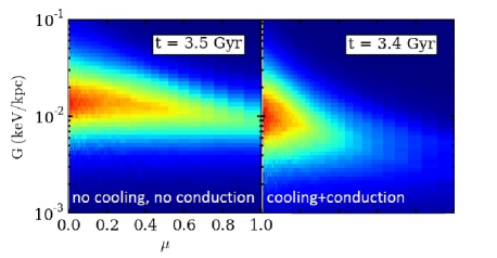
Figure 10: Joint PDF of $G$ and $\mu$ in a global cluster simulations. Left panel: same case as in Fig. 9. Right panel: identical case except with anisotropic conduction and radiative cooling switched on (Run SCX1 of ZuHone et al. 2013).

5 Conclusions

We have studied the correlations between the local fluctuating temperature gradients and the orientation of the frozen-in magnetic-field lines in the turbulent ICM. We have argued that the mutual orientation between isotherms and magnetic-field lines is not random, but rather a strong alignment is expected: gas motions tend to increase the temperature gradients and, at the same time, align the field lines perpendicular to the gradients. Cold fronts in clusters provide a vivid example of this process on large scales. The net result of the correlated evolution of the temperature distribution and the magnetic field is the effective suppression of the local heat flux. We note that global thermal conduction defined by radial temperature profiles of galaxy clusters (wich is one of the possible solutions to the cooling flow problem) is beyond the scope of this work.

We have calculated explicitly the joint distribution function of the gradients and the angles they make relative to the field lines and demonstrated that significant suppression takes place for generic 3D isotropic incompressible motions. The main conclusions are as follows:

• Strong correlation of the fluctuating temperature gradients and the local magnetic field orientation is established on the timescale of the turbulent eddy turnover.

• On average, the decay rate of temperature fluctuations is anti-correlated with the degree of amplification of the magnetic field by the gas motions. Volume averaged decay rate decreases with the growth of the magnetic-energy density as $\langle B^{2}\rangle^{-1/5}$.
  

  For disturbed clusters, where large-scale clumps of gas are displaced, the largest observed local gradients should be associated with the largest heat flux suppression. The estimates of the effective conductivity based on these gradients may not be characteristic of the bulk of the gas. This conclusion appears to be supported by global dynamic cluster simulations with and without anisotropic conduction.

Appendix A Statistical calculation of the joint PDF of $\mu$, $G$ and $B$

The general form of the joint PDF of the magnetic field and the temperature gradient is

$$P(\mn@boldsymbol{g},\mn@boldsymbol{b},G,B;t)=\langle\tilde{P}\rangle,$$

$$\tilde{P}=\delta(\mn@boldsymbol{g}-\mn@boldsymbol{g}(t))\delta(\mn@boldsymbol{b}-\mn@boldsymbol{b}(t))\delta(G-G(t))\delta(B-B(t)),$$ (47)

where $\mn@boldsymbol{g}$, $\mn@boldsymbol{b}$, $G$ and $B$ are variables and $\mn@boldsymbol{g}(t)$, $\mn@boldsymbol{b}(t)$, $G(t)$ and $B(t)$ are stochastic processes that are solutions of equations (3.5). Taking time derivative of $\tilde{P}$ and using equations (3.5), we obtain

$$\partial_{t}P=\mathrm{\hat{L}}^{m}_{i}\sigma^{i}_{m}\tilde{P},$$ (48)

where

$$\hat{\mathrm{L}}^{m}_{i}=\frac{\partial}{\partial g^{k}}(\delta^{k}_{m}-g^{k}g^{m})g^{i}-\frac{\partial}{\partial b^{k}}(\delta^{k}_{i}-b^{k}b^{i})b^{m}$$ (49)

$$+\frac{\partial}{\partial G}g^{i}g^{m}G-\frac{\partial}{\partial B}b^{i}b^{m}B.$$

The average of equation (48) is

$$\partial_{t}P=\mathrm{\hat{L}}^{m}_{i}\langle\sigma^{i}_{m}\tilde{P}\rangle$$ (50)

and we now apply the Furutsu-Novikov formula (Furutsu, 1963; Novikov, 1965) to calculate the right-hand side:

$$\langle\sigma^{i}_{m}(t)\tilde{P}(t)\rangle=\int\mathrm{d}t^{\prime}\langle\sigma^{i}_{m}(t)\sigma^{j}_{n}(t^{\prime})\rangle\bigg{\langle}\frac{\delta\tilde{P}(t)}{\delta\sigma^{j}_{n}(t^{\prime})}\bigg{\rangle}$$ (51)

$$=\kappa T^{ij}_{mn}\bigg{\langle}\frac{\delta\tilde{P}(t)}{\delta\sigma^{j}_{n}(t)}\bigg{\rangle}$$

where we have used equation (15). From equation (48),

$$\frac{\delta\tilde{P}(t)}{\delta\sigma^{j}_{n}(t)}=\int_{-\infty}^{t}\mathrm{d}t^{\prime}\bigg{[}\mathrm{\hat{L}}^{m}_{i}\delta^{i}_{j}\delta^{n}_{m}\delta(t-t^{\prime})\tilde{P}(t^{\prime})$$ (52)

$$+\mathrm{\hat{L}}^{m}_{i}\sigma^{i}_{m}(t^{\prime})\frac{\delta\tilde{P}(t^{\prime})}{\delta\sigma^{j}_{n}(t)}\bigg{]}=\frac{1}{2}\mathrm{\hat{L}}^{n}_{j}\tilde{P}(t).$$

The second term inside the integral vanishes by causality ($t^{\prime}<t$). Using equation (52) in equation (51) and substituting into equation (50), we arrive at a closed equation for the desired PDF:

$$\partial_{t}P=\frac{\kappa}{2}T^{ij}_{mn}\mathrm{\hat{L}}^{m}_{i}\mathrm{\hat{L}}^{n}_{j}P.$$ (53)

Since the medium is isotropic, the PDF only depends on $G$, $B$ and the angle between the unit vectors $\mn@boldsymbol{g}$ and $\mn@boldsymbol{b}$. Therefore, it can be factorized as

$$P(\mn@boldsymbol{g},\mn@boldsymbol{b},G,B;t)=\frac{1}{8\pi^{2}}\delta(\mn@boldsymbol{g}^{2}-1)\delta(\mn@boldsymbol{b}^{2}-1)p(\mu,G,B;t),$$ (54)

where $\mu=\mn@boldsymbol{b}\cdot\mn@boldsymbol{g}$. The factor $1/8\pi^{2}$ has been introduced in order to keep $p(\mu,G,B;t)$ normalized to unity. Substituting this expression into equation (53), we get

$$\mathrm{\hat{L}}^{m}_{i}\mathrm{\hat{L}}^{n}_{j}P=\delta(\mn@boldsymbol{g}^{2}-1)\delta(\mn@boldsymbol{b}^{2}-1)$$ (55)

$$\times\{(b^{i}b^{j}b^{m}b^{n}+g^{i}g^{j}g^{m}g^{n}-g^{i}b^{j}g^{m}b^{n}$$

$$-b^{i}g^{j}b^{m}g^{n})\mu\partial_{\mu}\mu\partial_{\mu}$$

$$+(b^{i}g^{j}b^{m}g^{n}-g^{i}g^{j}g^{m}g^{n})\mu\partial_{\mu}\partial_{G}G$$

$$+(g^{i}b^{j}g^{m}b^{n}-2b^{i}b^{j}b^{m}b^{n}+b^{i}g^{j}b^{m}g^{n})\mu\partial_{\mu}\partial_{B}B$$

$$-(g^{i}b^{j}g^{m}b^{n}+b^{i}g^{j}b^{m}g^{n})\partial_{G}G\partial_{B}B$$

$$+g^{i}g^{j}g^{m}g^{n}\partial_{G}G\partial_{G}G$$

$$+[2(d+1)(b^{i}b^{j}b^{m}b^{n}+g^{i}g^{j}g^{m}g^{n})$$

$$-2d(g^{i}b^{j}g^{m}b^{n}+b^{i}g^{j}b^{m}g^{n})-b^{m}b^{n}\delta^{i}_{j}-b^{j}b^{m}\delta^{i}_{n}$$

$$-g^{i}g^{n}\delta^{j}_{m}-g^{i}g^{j}\delta^{m}_{n}]\mu\partial_{\mu}$$

$$+[-2(d+1)g^{i}g^{j}g^{m}g^{n}+d(g^{i}b^{j}g^{m}b^{n}+b^{i}g^{j}b^{m}g^{n})$$

$$+g^{i}g^{n}\delta^{j}_{m}+g^{i}g^{j}\delta^{m}_{n}]\partial_{G}G$$

$$+[-2(d+1)b^{i}b^{j}b^{m}b^{n}+dg^{i}b^{j}g^{m}b^{n}+db^{i}g^{j}b^{m}g^{n}$$

$$+b^{m}b^{n}\delta^{i}_{j}+b^{j}b^{m}\delta^{j}_{m}]\partial_{B}B$$

$$+d[(d+2)(b^{i}b^{j}b^{m}b^{n}+g^{i}g^{j}g^{m}g^{n})-d(g^{i}b^{j}g^{m}b^{n}$$

$$+b^{i}g^{j}b^{m}g^{n})$$

$$-(b^{m}b^{n}\delta^{i}_{j}+b^{j}b^{m}\delta^{i}_{n}+g^{i}g^{n}\delta^{j}_{m}+g^{i}g^{j}\delta^{m}_{n})]\}p,$$

where $d$ is the number of spatial dimensions. The PDF is factorized, as it ought to be, and we only need to solve the equation for $p(\mu,G,B;t)$. Substituting equation (55) into equation (53), we perform the convolutions involving $T^{ij}_{mn}$ [see equation (16)] using the identities

$$T^{ij}_{mn}b^{i}b^{j}b^{m}b^{n}=\frac{d-1}{d+1},$$

$$T^{ij}_{mn}g^{i}b^{j}g^{m}b^{n}=\frac{\mu^{2}-1}{d+1},$$

$$T^{ij}_{mn}b^{j}b^{m}\delta^{i}_{n}=0,$$

$$T^{ij}_{mn}b^{m}b^{n}\delta^{i}_{j}=\frac{(d-1)(d+2)}{d+1},$$

$$T^{ij}_{mn}b^{i}g^{j}b^{m}g^{n}=\frac{\mu^{2}-1}{d+1},$$

$$T^{ij}_{mn}g^{i}g^{j}g^{m}g^{n}=\frac{d-1}{d+1},$$

$$T^{ij}_{mn}g^{i}g^{n}\delta^{j}_{m}=0,$$

$$T^{ij}_{mn}g^{i}g^{j}\delta^{m}_{n}=\frac{(d-1)(d-2)}{d+1}.$$ (56)

The result is equation (31).

References

- Albright et al. (2001) Albright B. J., Chandran B. D. G., Cowley S. C., Loh M., 2001, Phys. Plasmas, 8, 777
- Asai et al. (2007) Asai N., Fukuda N., Matsumoto R., 2007, ApJ, 663, 816
- Balbus (2000) Balbus S. A., 2000, ApJ, 534, 420
- Balkovsky & Fouxon (1999) Balkovsky E., Fouxon A., 1999, Phys. Rev. E, 60, 4164
- Bogdanović et al. (2009) Bogdanović T., Reynolds C. S., Balbus S. A., Parrish I. J., 2009, ApJ, 704, 211
- Boldyrev & Cattaneo (2004) Boldyrev S., Cattaneo F., 2004, Phys. Rev. Lett., 92, 144501
- Boldyrev & Schekochihin (2000) Boldyrev S. A., Schekochihin A. A., 2000, Phys. Rev. E, 62, 545
- Braginskii (1965) Braginskii S. I., 1965, Rev. Plasma Phys., 1, 205
- Chandran & Cowley (1998) Chandran B. D. G., Cowley S. C., 1998, Phys. Rev. Lett., 80, 3077
- Chandran et al. (1999) Chandran B. D. G., Cowley S. C., Ivanushkina M., Sydora R., 1999, ApJ, 525, 638
- Chandran & Maron (2004) Chandran B. D. G., Maron J. L., 2004, ApJ, 602, 170
- Chertkov et al. (1999) Chertkov M., Falkovich G., Kolokolov I., Vergassola M., 1999, Phys. Rev. Lett., 83, 4065
- Churazov et al. (2008) Churazov E., Forman W., Vikhlinin A., Tremaine S., Gerhard O., Jones C., 2008, MNRAS, 388, 1062
- Churazov & Inogamov (2004) Churazov E., Inogamov N., 2004, MNRAS, 350, L52
- Churazov et al. (2012) Churazov E., Vikhlinin A., Zhuravleva I., Schekochihin A., Parrish I., Sunyaev R., Forman W., Böhringer H., Randall S., 2012, MNRAS, 421, 1123
- Ettori & Fabian (2000) Ettori S., Fabian A. C., 2000, MNRAS, 317, L57
- Furutsu (1963) Furutsu K., 1963, J. Res. NBS, 67D, 303
- Inogamov & Sunyaev (2003) Inogamov N. A., Sunyaev R. A., 2003, Astron. Lett., 29, 791
- Kazantsev (1968) Kazantsev A. P., 1968, Soviet Phys. JETP, 26, 1031
- Kunz et al. (2012) Kunz M. W., Bogdanović T., Reynolds C. S., Stone J. M., 2012, ApJ, 754, 122
- Kunz et al. (2011) Kunz M. W., Schekochihin A. A., Cowley S. C., Binney J. J., Sanders J. S., 2011, MNRAS, 410, 2446
- Lau et al. (2009) Lau E. T., Kravtsov A. V., Nagai D., 2009, ApJ, 705, 1129
- Lyutikov (2006) Lyutikov M., 2006, MNRAS, 373, 73
- Malyshkin & Kulsrud (2001) Malyshkin L., Kulsrud R., 2001, ApJ, 549, 402
- Markevitch et al. (2003) Markevitch M., Mazzotta P., Vikhlinin A., Burke D., Butt Y., David L., Donnelly H., Forman W. R., Harris D., Kim D.-W., Virani S., Vrtilek J., 2003, ApJ, 586, L19
- Markevitch & Vikhlinin (2007) Markevitch M., Vikhlinin A., 2007, Phys. Rep., 443, 1
- McCourt et al. (2011) McCourt M., Parrish I. J., Sharma P., Quataert E., 2011, MNRAS, 413, 1295
- Mogavero & Schekochihin (2013) Mogavero F., Schekochihin A. A., 2013, ArXiv: 1312.3672
- Narayan & Medvedev (2001) Narayan R., Medvedev M. V., 2001, ApJ, 562, L129
- Novikov (1965) Novikov E., 1965, Soviet Phys. JETP, 20, 1290
- Parrish et al. (2009) Parrish I. J., Quataert E., Sharma P., 2009, ApJ, 703, 96
- Quataert (2008) Quataert E., 2008, ApJ, 673, 758
- Rechester & Rosenbluth (1978) Rechester A. B., Rosenbluth M. N., 1978, Phys. Rev. Lett., 40, 38
- Roediger et al. (2011) Roediger E., Brüggen M., Simionescu A., Böhringer H., Churazov E., Forman W. R., 2011, MNRAS, 413, 2057
- Rosner & Tucker (1989) Rosner R., Tucker W. H., 1989, ApJ, 338, 761
- Ruszkowski et al. (2011) Ruszkowski M., Lee D., Brüggen M., Parrish I., Oh S. P., 2011, ApJ, 740, 81
- Ruszkowski & Oh (2010) Ruszkowski M., Oh S. P., 2010, ApJ, 713, 1332
- Schekochihin et al. (2002) Schekochihin A., Cowley S., Maron J., Malyshkin L., 2002, Phys. Rev. E, 65, 016305
- Schekochihin & Cowley (2006) Schekochihin A. A., Cowley S. C., 2006, Phys. Plasmas, 13, 056501
- Schekochihin et al. (2004) Schekochihin A. A., Cowley S. C., Taylor S. F., Maron J. L., McWilliams J. C., 2004, ApJ, 612, 276
- Schekochihin et al. (2004) Schekochihin A. A., Haynes P. H., Cowley S. C., 2004, Phys. Rev. E, 70, 046304
- Schuecker et al. (2004) Schuecker P., Finoguenov A., Miniati F., Böhringer H., Briel U. G., 2004, A&A, 426, 387
- Sharma et al. (2009) Sharma P., Chandran B. D. G., Quataert E., Parrish I. J., 2009, ApJ, 699, 348
- Skilling et al. (1974) Skilling J., McIvor I., Holmes J. A., 1974, MNRAS, 167, 87P
- Subramanian et al. (2006) Subramanian K., Shukurov A., Haugen N. E. L., 2006, MNRAS, 366, 1437
- Tao (1995) Tao L., 1995, MNRAS, 275, 965
- Vikhlinin et al. (2001) Vikhlinin A., Markevitch M., Murray S. S., 2001, ApJ, 549, L47
- Xiang et al. (2007) Xiang F., Churazov E., Dolag K., Springel V., Vikhlinin A., 2007, MNRAS, 379, 1325
- Zhuravleva et al. (2011) Zhuravleva I. V., Churazov E. M., Sazonov S. Y., Sunyaev R. A., Dolag K., 2011, Astron. Lett., 37, 141
- ZuHone et al. (2011) ZuHone J. A., Markevitch M., Lee D., 2011, ApJ, 743, 16
- ZuHone et al. (2013) ZuHone J. A., Markevitch M., Ruszkowski M., Lee D., 2013, ApJ, 762, 69