Pricing approximations and error estimates for local Lévy-type models with default

Abstract

We find approximate solutions of partial integro-differential equations, which arise in financial models when defaultable assets are described by general scalar Lévy-type stochastic processes. We derive rigorous error bounds for the approximate solutions. We also provide numerical examples illustrating the usefulness and versatility of our methods in a variety of financial settings.

Keywords: Partial integro-differential equation, Asymptotic expansion, Pseudo-differential calculus, Option pricing, Lévy-type process, Defaultable asset

1 Introduction

It is now clear from empirical examinations of option prices and high-frequency data that asset prices exhibit jumps (see, e.g., Ait-Sahalia and Jacod (2012); Eraker (2004) and references therein). From a modeling perspective, the above evidence supports the use of exponential Lévy models, which are able to incorporate jumps in the price process through a Poisson random measure. Moreover, exponential Lévy models are convenient for option pricing since, for a wide variety of Lévy measures, the characteristic function of Lévy processes are known in closed-form, allowing for fast computation of option prices via generalized Fourier transforms (see Lewis (2001); Lipton (2002); Boyarchenko and Levendorskii (2002); Cont and Tankov (2004); Almendral and Oosterlee (2005)). However, a major disadvantage of exponential Lévy models is that they are spatially homogeneous; neither the drift, volatility nor the jump-intensity have any local dependence. Thus, exponential Lévy models are not able to exhibit volatility clustering or capture the leverage effect, both of which are well-known features of equity markets.

In addressing the above shortcomings, it is natural to allow the drift, diffusion and Lévy measure of a Lévy process to depend locally on the value of the underlying process. Compared to their Lévy counterparts, local Lévy models (also known as scalar Lévy-type models) are able to more accurately mimic the real-world dynamics of assets. However, the increased realism of local Lévy models is matched by an increased computational complexity; very few local Lévy models allow for efficiently computable exact option prices (the notable exception being the Lévy-subordinated diffusions considered in Mendoza-Arriaga et al. (2010)). Since an option price can directly related to the solution of a partial integro-differential equation (Kolmogorov backward equation) by means of the Feynman-Kac formula, other classical numerical approaches, such as finite difference or Monte Carlo methods, can be employed. However, such approaches are by no means free of drawbacks (see, for instance, Andersen and Andreasen (2000); d’Halluin et al. (2005)).

Recently, there have been a number of methods proposed for finding approximate option prices in local Lévy settings. We mention in particular the work of Benhamou et al. (2009), who use Malliavin calculus methods to derive analytic approximations for options prices in a setting that includes local volatility and Poisson jumps. We also mention the work of Jacquier and Lorig (2013), who use regular perturbation methods to derive option price and implied volatility approximations in a local-Lévy setting. Another polynomial operator expansion technique was proposed in Pagliarani and Pascucci (2013) and Pagliarani et al. (2013) to compute option prices in stochastic-local-Lévy volatility models.

More recently, Lorig, Pagliarani, and Pascucci (2014c) illustrate how to obtain a family of asymptotic approximations for the transition density of the full class of scalar Lévy-type process (including infinite activity Lévy-type processes). The methods developed in Lorig et al. (2014c) can be briefly described as follows. First, one considers the infinitesimal generator of a general scalar Lévy-type process. One expands the drift, volatility and killing coefficients as well as the Lévy kernel as an infinite series of analytic basis functions. The infinitesimal generator can then be formally written as an infinite series, with each term in the series corresponding to a different basis function. Inserting the expansion for the generator into the Kolmogorov backward equation, one obtains a sequence of nested Cauchy problems for the density of the Lévy-type process.

The polynomial expansion technique described in Lorig et al. (2014c) has also been applied in multi-dimensional settings. In particular, Lorig et al. (2014b) derive explicit approximations and error bounds for implied volatilities for a general class of $d$-dimensional diffusions. Lorig et al. (2013) derive error bounds for transition densities and option prices in a general $d$-dimensional diffusion setting. However, in neither of these papers do the authors consider processes with jumps. For $d$-dimensional models with jumps, Lorig et al. (2014a) derive explicit approximations for transition densities and option prices. However, the results are only formal, as no rigorous error bounds are established for the approximation. The main contribution of this paper is a rigorous proof of short-time error estimates on transition densities and option prices, under Local Lévy models with Gaussian jumps. Furthermore, the proof, which is based on a non-trivial generalization of the standard parametrix method, paves the road for further extensions in order to include more general choices of Lévy measures.

The main contributions of this paper are as follows. First, we analytically solve the sequence of nested Cauchy problems mentioned above and thereby derive an explicit expression of the approximate option price (i.e., solution of the integro-differential equation) to arbitrarily high order. Second, we provide a rigorous and detailed proof of some pointwise error estimates for the approximation. These estimates were announced, without proof, in Lorig et al. (2014c). Lastly, we illustrate how to implement our approximation formulas in Mathematica, Wolfram’s symbolic computation software. In particular, we provide numerical examples for transition densities, Call and Put prices, implied volatilities, bond prices and credit spreads. For the readers’ convenience, example Mathematica code is also made freely available on the authors’ websites. The numerical tests in this manuscript and the authors’ websites clearly demonstrate the versatility and accuracy of the method.

The rest of this paper proceeds as follows: in Section 2 we describe a financial market in which a defaultable asset evolves as an exponential Lévy-type process. We then relate the problem of the pricing of a European-style option to the solution of a partial integro-differential equation (PIDE). Next, in Section 3, we introduce a family of asymptotic solutions of the pricing PIDE. The main results are given in Sections 4, where global error bounds are proved for both the density and price approximations (Theorem 4.4 and Corollary 4.7. respectively). In addition to their practical use, these estimates are interesting from the theoretical point, as they imply some non-classical upper bounds for the fundamental solution of a certain class of integro-differential operators with variable coefficients. The proof of Theorem 4.4 is postponed to Section 6. Before proving the theorem, we provide in Section 5 a number of numerical examples, which are relevant for financial applications.

2 Market model and option pricing

For simplicity, we assume a frictionless market, no arbitrage, zero interest rates and no dividends. Our results can easily be extended to include locally dependent interest rates and dividends. We take, as given, an equivalent martingale measure $\mathbb{Q}$, chosen by the market on a complete filtered probability space $(\Omega,\mathscr{F},\{\mathscr{F}_{t},t\geq 0\},\mathbb{Q})$ satisfying the usual hypotheses. All stochastic processes defined below live on this probability space and all expectations are taken with respect to $\mathbb{Q}$. We consider a defaultable asset $S$ whose risk-neutral dynamics are given by

$$\begin{cases}S_{t}=\mathbb{I}_{\{\zeta>t\}}e^{X_{t}},\\ dX_{t}=\mu(t,X_{t})dt+\sigma(t,X_{t})dW_{t}+\int_{\mathbb{R}}z\tilde{N}(dt,X_{t-},dz),\\ \tilde{N}(dt,X_{t-},dz)=N(dt,X_{t-},dz)-\nu(t,X_{t-},dz)dt,\\ \zeta=\inf\left\{t\geq 0:\int_{0}^{t}\gamma(s,X_{s})ds\geq\mathscr{E}\right\}.\end{cases}$$ (2.1)

Here, $X$ is a Lévy-type process with local drift function $\mu(t,x)$, local volatility function $\sigma(t,x)\geq 0$ and state-dependent Poisson random and Lévy measures $N(dt,x,dz)$ and $\nu(t,x,dz)$ respectively. The random variable $\mathscr{E}\sim\text{Exp}(1)$ has an exponential distribution and is independent of $X$. Note that $\zeta$, which represents the default time of $S$, is defined here through the so-called canonical construction (see Bielecki and Rutkowski (2001)). This way of modeling default is also considered in a local volatility setting in Carr and Linetsky (2006); Linetsky (2006), and for exponential Lévy models in Capponi et al. (2013). Notice that the drift coefficient $\mu$ is fixed by $\sigma$, $\nu$ and $\gamma$ in order to satisfy the martingale condition:

$$\mu(t,x) =\gamma(t,x)-a(t,x)-\int_{\mathbb{R}}\nu(t,x,dz)(e^{z}-1-z), a(t,x) :=\frac{1}{2}\sigma^{2}(t,x).$$ (2.2)

We assume that the coefficients are measurable in $t$ and suitably smooth in $x$ so as to ensure the existence of a strong solution to (2.1) (see, for instance, Oksendal and Sulem (2005), Theorem 1.19). We also assume that

$$\bar{\nu}(dz) :=\sup_{(t,x)\in\mathbb{R}^{+}\times\mathbb{R}}\nu(t,x,dz),$$ (2.3)

satisfies the following three boundedness conditions

$$\int_{\mathbb{R}}\min\{|z|,z^{2}\}\,\bar{\nu}(dz) <\infty, \int_{|z|\geq 1}e^{z}\,\bar{\nu}(dz) <\infty,$$ (2.4)

which is rather standard assumption for financial applications. We will relax some of these assumptions for the numerical examples provided in Section 5. Even without the above assumptions in force, our numerical tests indicate that our approximation techniques gives very accurate results.

We consider a European derivative expiring at time $T$ with payoff $H(S_{T})$ and we denote by $V$ its price process. we introduce

$$h(x) :=H(e^{x})\qquad\text{and}\qquad K:=H(0).$$ (2.5)

Then, by no-arbitrage arguments (see, for instance, Linetsky (2006, Section 2.2)) the price of the option at time $t<T$ is given by

$$V_{t} =K+\mathbb{I}_{\{\zeta>t\}}\mathbb{E}\left[e^{-\int_{t}^{T}\gamma(s,X_{s})ds}\left(h(X_{T})-K\right)|X_{t}\right], t \leq T.$$ (2.6)

From (2.6) we see that, in order to compute the price of an option, we must evaluate functions of the form

$$u(t,x) :=\mathbb{E}\left[e^{-\int_{t}^{T}\gamma(s,X_{s})ds}h(X_{T})|X_{t}=x\right].$$ (2.7)

By a direct application of the Feynman-Kac representation theorem (see, for instance, Theorem 14.50 in Pascucci (2011)) the classical solution of the following Cauchy problem,

$$\begin{cases}(\partial_{t}+\mathscr{A})u(t,x)=0,\qquad&t\in[0,T[,\ x\in\mathbb{R},\\ u(T,x)=h(x),&x\in\mathbb{R},\end{cases}$$ (2.8)

when it exists, is equal to the function $u$ defined in (2.7). Here $\mathscr{A}\equiv\mathscr{A}(t,x)$ is the integro-differential operator associated with the SDE (2.1) and defined explicitly as

$$\mathscr{A}(t,x)f(x) =a(t,x)\partial_{xx}f(x)+{\mu}(t,x)\partial_{x}f(x)-\gamma(t,x)f(x)$$ (2.9)

$$\qquad+\int_{\mathbb{R}}\left(f(x+z)-f(x)-z\partial_{x}f(x)\right)\nu(t,x,dz)$$ (2.10)

with ${\mu}$ and $a$ as in (2.2). We say that $\mathscr{A}$ is the characteristic operator of $X_{t}$.

Sufficient conditions for the existence and uniqueness of a classical solution of a second order elliptic integro-differential equations of the form (2.8) are given in Theorem II.3.1 of Garroni and Menaldi (1992). In particular, given the existence of the fundamental solution $p(t,x;T,y)$ of $\left(\partial_{t}+\mathscr{A}\right)$, we have that for any integrable datum $h$, the Cauchy problem (2.8) has a classical solution that can be represented as

$$u(t,x) =\int_{\mathbb{R}}h(y)p(t,x;T,y)dy.$$ (2.11)

Notice that $p(t,x;T,y)$ is a “defective” probability density since (due to the possibility that $S_{T}=0$) we have

$$\int_{\mathbb{R}}p(t,x;T,y)dy\leq 1.$$ (2.12)

3 Approximate densities and option prices via polynomial expansions

In this section we describe the approximation methodology and define the notation that will be needed in subsequent sections.

Definition 3.1.

For any $n\leq N\in\mathbb{N}_{0}$, let $a_{n}=a_{n}(t,x)$, $\gamma_{n}=\gamma_{n}(t,x)$ and $\nu_{n}=\nu_{n}(t,x,dz)$ be such that the following hold:

1. For any $t\in[0,T]$, the functions $a_{n}(t,\cdot)$, $\gamma_{n}(t,\cdot)$ are polynomials with $a_{0}(t,x)\equiv a_{0}(t)$, $\gamma_{0}(t,x)\equiv\gamma_{0}(t)$, and for any $x\in\mathbb{R}$ the functions $a_{n}(\cdot,x)$, $\gamma_{n}(\cdot,x)$ belong to $L^{\infty}([0,T])$.

2. For any $t\in[0,T]$, $x\in\mathbb{R}$, we have

   $$\nu_{n}(t,x,dz) =\sum_{m=0}^{M_{n}}x^{m}\nu_{n,m}(t,dz), M_{n} \in\mathbb{N}_{0},$$ (3.1)

   where each $\nu_{n,m}(t,dz)$ satisfies condition (2.4). Moreover, $M_{0}=0$, $\nu_{0}\geq 0$ and

   $$\int_{|z|\geq 1}e^{\lambda|z|}\nu_{0}(t,dz)<\infty,\qquad t\in[0,T],$$ (3.2)

   for some positive $\lambda$.

Then we say that $\left(\mathscr{A}_{n}(t)\right)_{0\leq n\leq N}$, defined by

$$\mathscr{A}_{n}(t,x)f(x) =a_{n}(t,x)(\partial_{xx}f(x)-\partial_{x}f(x))+\gamma_{n}(t,x)\left(\partial_{x}f(x)-f(x)\right)$$ (3.3)

$$\quad+\sum_{m=1}^{M_{n}}x^{m}\left(-\int_{\mathbb{R}}(e^{z}-1-z)\,\nu_{n,m}(t,dz)\,\partial_{x}f(x)+\int_{\mathbb{R}}\left(e^{z\,\partial_{x}}-1-z\,\partial_{x}\right)f(x)\,\nu_{n,m}(t,dz)\right)$$ (3.4)

$$\equiv a_{n}(t,x)(\partial_{xx}f(x)-\partial_{x}f(x))+\gamma_{n}(t,x)\left(\partial_{x}f(x)-f(x)\right)$$ (3.5)

$$\quad-\int_{\mathbb{R}}(e^{z}-1-z)\,\nu_{n}(t,x,dz)\,\partial_{x}f(x)+\int_{\mathbb{R}}(f(x+z)-f(x)-z\partial_{x}f(x))\,\nu_{n}(t,x,dz),$$ (3.6)

is an $N$-th order polynomial expansion of $\mathscr{A}(t)$.

Definition 3.1 allows for very general polynomial specifications. The idea is to choose an expansion $(\mathscr{A}_{n}(t))$ that closely approximates $\mathscr{A}(t)$, i.e. formally one has

$$\mathscr{A}(t,x)=\sum_{n=0}^{\infty}\mathscr{A}_{n}(t,x).$$ (3.7)

The precise sense of this approximation will depend on the application. Below, we present three polynomial expansions. The first two expansion schemes provide an accurate approximation $\mathscr{A}(t,x)$ in a pointwise local sense, under the assumption of smooth coefficients. The last expansion scheme approximates $\mathscr{A}(t,x)$ in a global sense and can be applied even in the case of discontinuous coefficients.

Example 3.2.

(Taylor polynomial expansion)
Assume the coefficients $a(t,\cdot),\gamma(t,\cdot)\in C^{N}(\mathbb{R})$ and that the compensator $\nu$ takes the form

$$\nu(t,x,dz)=h(t,x,z)\bar{\nu}(dz)$$

where $h(t,\cdot,z)\in C^{N}(\mathbb{R})$ with $h\geq 0$, and $\bar{\nu}$ is a Lévy measure. Then, for any fixed $\bar{x}\in{\mathbb{R}}$ and $n\leq N$, we define $a_{n}$, $\gamma_{n}$ and $\nu_{n}$ as the $n$th order term of the Taylor expansions of $a$, $\gamma$ and $\nu$ respectively in the spatial variables $x$ around the point $\bar{x}$. That is, we set

$$a_{n}(t,x)=\frac{\partial_{x}^{n}a(t,\bar{x})}{n!}(x-\bar{x})^{n},\qquad\gamma_{n}(t,x)=\frac{\partial_{x}^{n}\gamma(t,\bar{x})}{n!}(x-\bar{x})^{n},\qquad\nu_{n}(t,x,dz)=\frac{\partial_{x}^{n}h(t,\bar{x},z)}{n!}(x-\bar{x})^{n}\bar{\nu}(dz).$$ (3.8)

The expansion proposed in Lorig et al. (2014b) and Lorig et al. (2014d) is the particular case when $\nu\equiv 0$.

Example 3.3.

(Time-dependent Taylor polynomial expansion)
Under the assumptions of Example 3.2, fix a trajectory $\bar{x}:\mathbb{R}_{+}\to\mathbb{R}$. We then define $a_{n}$, $\gamma_{n}$ and $\nu_{n}$ as the $n$th order term of the Taylor expansions of $a$, $\gamma$ and $\nu$ respectively around $\bar{x}(t)$. This expansion for the coefficients allows the expansion point $\bar{x}$ of the Taylor series to evolve in time according to the evolution of the underlying process $X_{t}$. For instance, one could choose $\bar{x}(t)=\mathbb{E}[X_{t}]$. In Lorig et al. (2014b) this choice results in a highly accurate approximation for option prices and implied volatility in the Heston (1993) model, recently included in the open-source financial library QuantLib.

Example 3.4.

(Hermite polynomial expansion)
Hermite expansions can be useful when the diffusion coefficients are discontinuous. A remarkable example in financial mathematics is given by the Dupire’s local volatility formula for models with jumps (see Friz et al. (2013)). In some cases, e.g., the well-known Variance-Gamma model, the fundamental solution (i.e., the transition density of the underlying stochastic model) has singularities. In such cases, it is natural to approximate it in some $L^{p}$ norm rather than in the pointwise sense. For the Hermite expansion centered at $\bar{x}$, one sets

$$a_{n}(t,x) =\langle\mathbf{H}_{n}(\cdot-\bar{x}),a(t,\cdot)\rangle_{\Gamma}\mathbf{H}_{n}(x-\bar{x}),\qquad\gamma_{n}(t,x)=\langle\mathbf{H}_{n}(\cdot-\bar{x}),\gamma(t,\cdot)\rangle_{\Gamma}\mathbf{H}_{n}(x-\bar{x}),$$ (3.9)

$$\nu_{n}(t,x,dz) =\langle\mathbf{H}_{n}(\cdot-\bar{x}),\nu(t,\cdot,dz)\rangle_{\Gamma}\mathbf{H}_{n}(x-\bar{x}),$$ (3.10)

where the inner product $\langle\cdot,\cdot\rangle_{\Gamma}$ is an integral over $\mathbb{R}$ with a Gaussian weighting centered at $\bar{x}$ and $\mathbf{H}_{n}(x)$ is the $n$-th one-dimensional Hermite polynomial (properly normalized so that $\langle\mathbf{H}_{m},\mathbf{H}_{n}\rangle_{\Gamma}=\delta_{m,n}$ with $\delta_{m,n}$ being the Kronecker’s delta function).

Remark 3.5.

Although in each of the above examples, $a_{n}$, $\gamma_{n}$ and $\nu_{n}$ are polynomials in $x$ of degree $n$, this is not a requirement of our expansion method. The degree of $a_{n}$, $\gamma_{n}$ and $\nu_{n}$ may be greater than, equal to, or less than $n$.

We now return to Cauchy problem (2.8). Following the classical perturbation approach, we expand the solution $u$ as an infinite sum

$$u =\sum_{n=0}^{\infty}u_{n}.$$ (3.11)

Inserting (3.7) and (3.11) into (2.8) we find that the functions $(u_{n})_{n\geq 0}$ satisfy the following sequence of nested Cauchy problems

$$\begin{cases}(\partial_{t}+\mathscr{A}_{0})u_{0}(t,x)=0,\qquad&t\in[0,T[,\ x\in\mathbb{R},\\ u_{0}(T,x)=h(x),&x\in\mathbb{R},\end{cases}$$ (3.12)

and

$$\begin{cases}(\partial_{t}+\mathscr{A}_{0})u_{n}(t,x)=-\sum\limits_{k=1}^{n}\mathscr{A}_{k}(t,x)u_{n-k}(t,x),\qquad&t\in[0,T[,\ x\in\mathbb{R},\\ u_{n}(T,x)=0,&x\in\mathbb{R}.\end{cases}$$ (3.13)

Remark 3.6.

In fact, the nested sequence of Cauchy problems (3.12)-(3.13) satisfied by the sequence of functions $(u_{n})$ is a particular choice. This choice can be motivated by considering a family of Cauchy problems, indexed by a small parameter $\varepsilon$

$$(\partial_{t}+\mathscr{A}^{\varepsilon})u^{\varepsilon} =0, u^{\varepsilon}(T,x) =h(x), \mathscr{A}^{\varepsilon} =\sum_{n=0}^{\infty}\varepsilon^{n}\mathscr{A}_{n}, \varepsilon \in[0,1].$$ (3.14)

Note that, by (3.7), we formally have $\mathscr{A}^{\varepsilon}|_{\varepsilon=1}=\mathscr{A}$. If one seeks a solution to (3.14) of the form $u^{\varepsilon}=\sum_{n=0}^{\infty}\varepsilon^{n}u_{n}$, then, collecting terms of like powers of $\varepsilon$ one finds that $u_{0}$ and $u_{n}$ satisfy (3.13) and (3.13), respectively.

3.1 Expression for $u_{0}$

Notice that $\mathscr{A}_{0}=\mathscr{A}_{0}(t,x)$ is the characteristic operator of the following additive process

$$dX^{0}_{t}=\left(\gamma_{0}(t)-a_{0}(t)-\int_{\mathbb{R}}(e^{z}-1-z)\,\nu_{0}(t,dz)\right)dt+\sqrt{2a_{0}(t)}dW_{t}+\int_{\mathbb{R}}z\left(N^{(0)}_{t}(dt,dz)-\nu_{0}(t,dz)dt\right),$$ (3.15)

whose characteristic function $\hat{p}_{0}(t,x;T,\xi)$ is given explicitly by

$$\hat{p}_{0}(t,x;T,\xi) :=\mathbb{E}[e^{i\xi X_{T}^{0}}|X_{t}^{0}=x]=\exp\left(i\xi x+\mathbf{\Phi}_{0}(t,T,\xi)\right),$$ (3.16)

where

$$\mathbf{\Phi}_{0}(t,T,\xi)=\left(i\xi\,\mathbf{m}(t,T)-\frac{1}{2}\mathbf{C}(t,T)\xi^{2}+\mathbf{\Psi}(t,T,\xi)-\int_{t}^{T}{\gamma}_{0}(s)ds\right),$$ (3.17)

and with $\mathbf{m}(t,T)$, $\mathbf{C}(t,T)$ and $\mathbf{\Psi}(t,T,\xi)$ being defined as

$$\mathbf{m}(t,T) :=\int_{t}^{T}\left(\gamma_{0}(s)-a_{0}(s)-\int_{\mathbb{R}}(e^{z}-1-z)\,\nu_{0}(s,dz)\right)ds,$$ (3.18)

$$\mathbf{C}(t,T) :=\int_{t}^{T}2a_{0}(s)ds,$$ (3.19)

$$\mathbf{\Psi}(t,T,\xi) :=\int_{t}^{T}\int_{\mathbb{R}}(e^{iz\xi}-1-iz\xi)\,\nu_{0}(s,dz)ds.$$ (3.20)

Note, the additive process $X^{0}$ in (3.15) is assumed to be defined on an appropriate probability space. It is well-known that additive processes can be constructed as time-changed Lévy processes (see (Cont and Tankov, 2004, Chapter 14)). The fundamental solution $p_{0}$ of $\left({\partial}_{t}+\mathscr{A}_{0}\right)$, which exists if $a_{0}>0$ (Sato, 1999, Proposition 28.3), can be recovered by Fourier inversion since, by the first equality in (3.16), we have

$$\hat{p}_{0}(t,x;T,\xi)=\mathscr{F}_{y}p_{0}(t,x,;T,\cdot)(\xi):=\int_{\mathbb{R}}e^{iy\xi}p_{0}(t,x,;T,y)dy,$$ (3.21)

and therefore

$$p_{0}(t,x,;T,y) =\mathscr{F}_{y}^{-1}\hat{p}_{0}(t,x;T,\cdot)(y):=\frac{1}{2\pi}\int_{\mathbb{R}}e^{-iy\xi}\hat{p}_{0}(t,x;T,\xi)d\xi.$$ (3.22)

Given the fundamental solution $p_{0}(t,x,;T,y)$, we have the representation for the solution $u_{0}$ of problem (3.12)

$$u_{0}(t,x) =\int\limits_{\mathbb{R}}p_{0}(t,x;T,y)h(y)\,dy,\quad t<T,\ x\in\mathbb{R}.$$ (3.23)

Assume that the payoff function $h$ and its Fourier transform $\hat{h}(y)\in L^{1}(\mathbb{R},dy)$. Then, by inserting the expression (3.22) for $p_{0}(t,x,;T,y)$ into (3.23) and integrating with respect to $\xi$, we also have the following alternative representation

$$u_{0}(t,x) =\frac{1}{2\pi}\int\limits_{\mathbb{R}}\hat{p}_{0}(t,x;T,\xi)\hat{h}(-\xi)\,d\xi.$$ (3.24)

3.2 Expression for $u_{n}$

The following theorem provides an explicit formula for $u_{n}(t,x)$ in (3.13) expressed in terms of integro-differential operators applied to $u_{0}(t,x)$ in (3.23).

Theorem 3.7.

Fix $N\in\mathbb{N}$ and let $\left(\mathscr{A}_{n}(t)\right)_{0\leq n\leq N}$ be an $N$th order polynomial expansion of $\mathscr{A}$ as in Definition 3.1. For any $1\leq n\leq N$, we have

$$u_{n}(t,x)=\mathscr{L}^{x}_{n}(t,T)u_{0}(t,x),\quad t<T,\ x,\xi\in\mathbb{R},\qquad 1\leq n\leq N,$$ (3.25)

with $u_{0}$ as in (3.23) and

$$\mathscr{L}_{n}^{x}(s_{0},T):=\sum_{h=1}^{n}\int_{s_{0}}^{T}ds_{1}\int_{s_{1}}^{T}ds_{2}\cdots\int_{s_{h-1}}^{T}ds_{h}\sum_{i\in I_{n,h}}\mathscr{G}^{x}_{i_{1}}(s_{0},s_{1})\cdots\mathscr{G}^{x}_{i_{h}}(s_{0},s_{h}),$$ (3.26)

where

$$I_{n,h} =\{i=(i_{1},\dots,i_{h})\in\mathbb{N}^{h}\mid i_{1}+\dots+i_{h}=n\}, 1 \leq h\leq n,$$ (3.27)

and $\mathscr{G}^{x}_{n}(t,s)$ is the operator (see Remark 3.8 below)

$$\mathscr{G}^{x}_{n}(t,s) :=\mathscr{A}_{n}\left(s,\mathscr{M}^{x}(t,s)\right),$$ (3.28)

with $\mathscr{M}^{x}(t,s)$ acting as

$$\mathscr{M}^{x}(t,s)f(x)= \left(x+\mathbf{m}(t,s)+\mathbf{C}(t,s)\,\partial_{x}\right)f(x)+\int_{t}^{s}\int_{\mathbb{R}}\left(f(x+z)-f(x)\right)z\,\nu_{0}(r,dz)dr.$$ (3.29)

Remark 3.8.

The operator in (3.28) can be written more explicitly as

$$\mathscr{A}_{n}\left(s,\mathscr{M}^{x}(t,s)\right)f(x)= a_{n}(t,\mathscr{M}^{x}(t,s))(\partial_{xx}f(x)-\partial_{x}f(x))+\gamma_{n}(t,\mathscr{M}^{x}(t,s))\left(\partial_{x}f(x)-f(x)\right)$$ (3.30)

$$-\sum_{m=1}^{M_{n}}\big{(}\mathscr{M}^{x}(t,s)\big{)}^{m}\int_{\mathbb{R}}(e^{z}-1-z)\,\nu_{n,m}(t,dz)\,\partial_{x}f(x)$$ (3.31)

$$+\sum_{m=1}^{M_{n}}\big{(}\mathscr{M}^{x}(t,s)\big{)}^{m}\int_{\mathbb{R}}\big{(}f(x+z)-f(x)-z\partial_{x}f(x)\big{)}\nu_{n,m}(t,dz).$$ (3.32)

Remark 3.9.

Theorem 3.7 extends the novel representation given in (Lorig et al., 2013, Theorem 3.8), which is given for the purely diffusion case. When no jump component is present the operator $\mathscr{M}^{x}$ in (3.29) reduces to

$$\mathscr{M}^{x}(t,s)=x+\mathbf{m}(t,s)+\mathbf{C}(t,s)\,\partial_{x}.$$ (3.33)

Remark 3.10.

The expression for $u_{n}$ given in (3.25) can be used in two ways. First, if the fundamental solution $p_{0}(t,x;T,y)$ is explicitly available (this is always the case in the purely diffusive setting), then to obtain $u_{n}$ one can apply the operator $\mathscr{L}_{n}^{x}(t,T)$ directly to $p_{0}(t,x;T,y)$ in (3.23). Second, if $p_{0}(t,x;T,y)$ is not available explicitly, then one can obtain a Fourier representation for $u_{n}$ by applying the operator $\mathscr{L}_{n}^{x}(t,T)$ directly to $\hat{p}_{0}(t,x;T,\xi)$ in (3.24). The details of the latter approach will be shown in Subsection 3.2.1.

Proof of Theorem 3.7.

Let $p_{0}$ be formally defined by (3.21). The proof of Theorem 3.7 relies on the following symmetry properties: for any $t<s$ and $x,y\in\mathbb{R}$, we have

$$p_{0}(t,x;s,y) =p_{0}(t,0;s,y-x),$$ (3.34)

$$\partial_{x}p_{0}(t,x;s,y) =-\partial_{y}p_{0}(t,x;s,y),$$ (3.35)

and

$$y\,p_{0}(t,x;s,y) =\mathscr{M}^{x}(t,s)p_{0}(t,x;s,y),$$ (3.36)

$$x\,p_{0}(t,x;s,y) =\bar{\mathscr{M}}^{y}(t,s)p_{0}(t,x;s,y),$$ (3.37)

with $\bar{\mathscr{M}}^{y}(t,s)$ acting as

$$\bar{\mathscr{M}}^{y}(t,s)f(y)= \left(y-\mathbf{m}(t,s)+\mathbf{C}(t,s)\partial_{y}\right)f(y)+\int_{t}^{s}\int_{\mathbb{R}}\left(f(y+z)-f(y)\right)z\nu_{0}(r,-dz)dr.$$ (3.38)

Identities (3.34)-(3.35) follow directly from the spatial-homogeneity of the coefficients of $\mathscr{A}_{0}$. In order to prove (3.36)-(3.37), we shall use some standard properties of the Fourier transform. For any function $f$ in the Schwartz space we have

$$i\xi\mathscr{F}_{x}(f)=\mathscr{F}_{x}(-\partial_{x}f),\qquad\mathscr{F}_{x}(xf)=-i\partial_{\xi}\mathscr{F}_{x}f,$$ (3.39)

and for any Lévy measure $\mathfrak{m}$ such that $\int_{|x|>1}|x|\,\mathfrak{m}(dx)<\infty$, we have

$$\mathscr{F}_{x}\left(\int_{\mathbb{R}}\left(f(x-z)-f(x)\right)z\,\mathfrak{m}(dz)\right)(\xi)=\int_{\mathbb{R}}(e^{iz\xi}-1)z\,\mathfrak{m}(dz)\,\mathscr{F}_{x}f(\xi).$$ (3.40)

Thus, by (3.39) we obtain

$$\mathscr{F}_{y}(y\,p_{0}(t,x;s,y))(\xi)$$ (3.41)

$$=-i\partial_{\xi}\mathscr{F}_{y}(p_{0}(t,x;s,y))(\xi)$$ (3.42)

$$=\left(x+\mathbf{m}(t,s)+\mathbf{C}(t,s)i\xi-i\partial_{\xi}\mathbf{\Psi}(t,s,\xi)\right)\mathscr{F}_{y}p_{0}(t,x;s,y)(\xi)$$ (by (3.16)-(3.17)) (3.43)

$$=\left(x+\mathbf{m}(t,s)+\mathbf{C}(t,s)i\xi+\int_{t}^{s}\int_{\mathbb{R}}(e^{iz\xi}-1)\,z\,\nu_{0}(r,dz)dr\right)\mathscr{F}_{y}p_{0}(t,x;s,y)(\xi)$$ (by (3.20)) (3.44)

$$=\mathscr{F}_{y}\left(\left(x+\mathbf{m}(t,s)-\mathbf{C}(t,s)\partial_{y}\right)p_{0}(t,x;s,y)\right)(\xi)$$ (3.45)

$$\quad+\mathscr{F}_{y}\left(\int_{t}^{s}\int_{\mathbb{R}}\left(p_{0}(t,x;s,y-z)-p_{0}(t,x;s,y)\right)\,\nu_{0}(r,dz)dr\right)(\xi)$$ (by (3.39) and (3.40)) (3.46)

$$=\mathscr{F}_{y}\left(\mathscr{M}^{x}(t,s)p_{0}(t,x;s,y)\right)(\xi).$$ (by (3.35), (3.34) and (3.29)) (3.47)

The identity (3.37) arises from the same arguments and because, by the symmetry property (3.34), we have

$$\mathscr{F}_{x}p_{0}(t,\cdot\,;T,y)(\xi)=\exp\left(i\xi(y-\mathbf{m}(t,T))-\frac{1}{2}\mathbf{C}(t,T)\xi^{2}+\mathbf{\Psi}(t,T,-\xi)-\int_{t}^{T}{\gamma}_{0}(s)ds\right).$$ (3.48)

As indicated in Remark 3.9, Theorem 3.7 reduces to (Lorig et al., 2013, Thorem 3.8) in case of a null Lévy measure $\nu(t,x,dz)\equiv 0$. The proof of the (Lorig et al., 2013, Thorem 3.8) is based on a systematic use of symmetry properties of Gaussian densities combined with some classical relations such as the Chapman-Kolmogorov equation and the Duhamel’s principle. Using the same classical relations, the proof of Theorem 3.7 follows by replacing the Gaussian symmetry properties in (Lorig et al., 2013, Lemma 5.4) with the symmetries properties (3.34)-(3.35)-(3.36)-(3.37) outlined above for additive processes. We refer to (Lorig et al., 2013, Section 5) for the details. ∎

3.2.1 Fourier representation for $u_{n}$

Using (3.16), (3.24) and (3.25), we obtain

$$u_{n}(t,x)=\mathscr{L}^{x}_{n}(t,T)u_{0}(t,x) =\frac{1}{2\pi}\int_{\mathbb{R}}e^{\mathbf{\Phi}_{0}(t,T,\xi)}\big{(}\mathscr{L}^{x}_{n}(t,T)e^{ix\xi}\big{)}\hat{h}(-\xi)d\xi.$$ (3.49)

The term in parenthesis $\mathscr{L}^{x}_{n}(t,T)e^{ix\xi}$ can be computed explicitly. However, $\mathscr{L}^{x}_{n}(t,T)$ is, in general, an integro-differential operator (when $X$ is a diffusion $\mathscr{L}^{x}_{n}(t,T)$ is simply a differential operator). Thus, for models with jumps, computing $\mathscr{L}^{x}_{n}(t,T)e^{ix\xi}$ is a challenge. Remarkably, we will show that there exists a differential operator $\hat{\mathscr{L}}^{\xi}_{n}(t,T)$ such that

$$\mathscr{L}^{x}_{n}(t,T)e^{ix\xi}=\hat{\mathscr{L}}^{\xi}_{n}(t,T)e^{ix\xi},$$ (3.50)

where, for clarity, we have explicitly indicated using the superscript $\xi$ that $\hat{\mathscr{L}}^{\xi}_{n}(t,T)$ acts on $\xi$. With a slight abuse of terminology, we call $\hat{\mathscr{L}}^{\xi}_{n}$ the symbol of the operator $\mathscr{L}_{n}^{x}(t,T)$ in (3.26).

Let us consider the operator $\mathscr{M}^{x}(t,s)$ in (3.29); its symbol $\widehat{\mathscr{M}}^{\xi}(t,s)$ is defined analogously to (3.50), i.e.

$$\mathscr{M}^{x}(t,s)e^{ix\xi}=\widehat{\mathscr{M}}^{\xi}(t,s)e^{ix\xi}.$$ (3.51)

Explicitly, we have

$$\widehat{\mathscr{M}}^{\xi}(t,s)=F(\xi,t,s)-i\partial_{\xi_{i}},$$ (3.52)

where the function $F$ is defined as

$$F(\xi,t,s) =-i\xi\mathbf{\Psi}(t,s,\xi)+\mathbf{m}(t,s)ds+i\xi\mathbf{C}(t,s)$$ (3.53)

$$=\int_{t}^{s}\int_{\mathbb{R}}z\left(e^{iz\xi}-1\right)\nu_{0}(\tau,dz)d\tau+\mathbf{m}(t,s)ds+i\xi\mathbf{C}(t,s).$$ (3.54)

We note that, while $\mathscr{M}^{x}$ is a first order integro-differential operator, its symbol $\widehat{\mathscr{M}}^{\xi}$ is a first order differential operator. For this reason, it is more convenient to use the symbol $\widehat{\mathscr{M}}^{\xi}$ instead of the operator $\mathscr{M}^{x}$. From identity (3.51) we obtain directly the expression of the symbol of $\mathscr{G}_{j}$ in (3.28). Indeed, recalling the expression (3.1) of $\nu_{j}$ we have

$$\hat{\mathscr{G}}^{\xi}_{j}(t,s) =-(\xi^{2}+i\xi)\,a_{n}\big{(}s,\widehat{\mathscr{M}}^{\xi}(t,s)\big{)}+\left(i\xi-1\right)\,\gamma_{n}\big{(}s,\widehat{\mathscr{M}}^{\xi}(t,s)\big{)}$$ (3.55)

$$\quad+\sum_{m=1}^{M_{n}}\left(-i\xi\int_{\mathbb{R}}(e^{z}-1-z)\,\nu_{n,m}(s,dz)+\int_{\mathbb{R}}\left(e^{iz\xi}-1-iz\xi\right)\nu_{n,m}(s,dz)\right)\left(\widehat{\mathscr{M}}^{\xi}(t,s)\right)^{m}.$$ (3.56)

Thus we have proved the following lemma

Lemma 3.11.

We have

$$\hat{\mathscr{L}}^{\xi}_{n}(t,T) =\sum_{k=1}^{n}\int_{t}^{T}dt_{1}\int_{t_{1}}^{T}dt_{2}\cdots\int_{t_{k-1}}^{T}dt_{k}\sum_{i\in I_{n,k}}\hat{\mathscr{G}}^{\xi}_{i_{1}}(t,t_{1})\hat{\mathscr{G}}^{\xi}_{i_{2}}(t,t_{2})\cdots\hat{\mathscr{G}}^{\xi}_{i_{k}}(t,t_{k}),$$ (3.57)

with $I_{n,k}$ as defined in (3.27).

The following theorem extends the Fourier pricing formula (3.24) to higher order approximations.

Theorem 3.12.

Assume that $h,\hat{h}\in L^{1}(\mathbb{R},dy)$. Then, for any $n\geq 1$ we have

$$u_{n}(t,x) =\frac{1}{2\pi}\int_{\mathbb{R}}\hat{p}_{n}(t,x,T,\xi)\hat{h}(-\xi)\,d\xi,$$ (3.58)

where $\hat{p}_{n}(t,x,T,\xi)$ is the $n$th order term of the approximation of the characteristic function of $X$. Explicitly, we have

$$\hat{p}_{n}(t,x,T,\xi):=\hat{p}_{0}(t,x,T,\xi)\left(e^{-ix\xi}\hat{\mathscr{L}}^{\xi}_{n}(t,T)e^{ix\xi}\right)$$ (3.59)

where $\hat{p}_{0}(t,x,T,\xi)$ is the $0$th order approximation in (3.16) and $\hat{\mathscr{L}}^{\xi}_{n}(t,T)$ is the differential operator defined in (3.57).

Proof.

We first note that, since the approximating operator $\mathscr{L}^{x}_{n}$ acts in the $x$ variables, then it commutes with the Fourier pricing operator (3.24). Thus, by (3.25) combined with (3.24), we get

$$u_{n}(t,x)=\mathscr{L}^{x}_{n}(t,T)u_{0}(t,x) =\frac{1}{2\pi}\int_{\mathbb{R}}\mathscr{L}^{x}_{n}(t,T)e^{ix\xi+\mathbf{\Phi}_{0}(t,T,\xi)}\hat{h}(-\xi)\,d\xi$$ (3.60)

$$=\frac{1}{2\pi}\int_{\mathbb{R}}\hat{p}_{0}(t,x,T,\xi)\left(e^{-ix\xi}\mathscr{L}^{x}_{n}(t,T)e^{ix\xi}\right)\hat{h}(-\xi)\,d\xi,$$ (3.61)

and the thesis follows from (3.50). ∎

Remark 3.13.

Computing the term in parenthesis above $\left(e^{-ix\xi}\hat{\mathscr{L}}^{\xi}_{n}(t,T)e^{ix\xi}\right)$ is a straightforward exercise since the symbol $\hat{\mathscr{L}}^{\xi}_{n}(t,T)$, given in (3.57), is a differential operator.

Example 3.14.

Let $(\mathscr{A}_{0},\mathscr{A}_{1})$ the $1$-st order Taylor expansion of $\mathscr{A}$ proposed in Example 3.2. Then we have

$$\hat{p}_{1}(t,x;T,\xi)=\hat{p}_{0}(t,x;T,\xi)\int_{t}^{T}\bar{\mathscr{A}}_{1}(s,\xi)\big{(}x-\bar{x}+\mathbf{m}(t,s)+i\xi\mathbf{C}(t,s)-i\partial_{\xi}\mathbf{\Psi}(t,s,\xi)\big{)}ds,$$ (3.62)

with

$$\bar{\mathscr{A}}_{1}(s,\xi) =\gamma_{1}(s)(i\xi-1)+a_{1}(s)(-\xi^{2}-i\xi)-i\xi\int_{\mathbb{R}}(e^{z}-1-z)\,\nu_{1}(s,dz)+\int_{\mathbb{R}}\left(e^{iz\xi}-1-iz\xi\right)\,h_{1}(s,\bar{x},z)\bar{\nu}(s,dz),$$ (3.63)

and

$$\gamma_{1}(s)=\partial_{x}\gamma(s,\bar{x}),\qquad a(s)=\partial_{x}a(s,\bar{x}),\qquad h_{1}(s,\bar{x},z)=\partial_{x}h(s,\bar{x},z).$$ (3.64)

Remark 3.15.

If $h(y)\notin L^{1}(\mathbb{R},dy)$ but $h(y)e^{cy}\in L^{1}(\mathbb{R},dy)$ for some $c\in\mathbb{R}$ (which is the case for Call and Put payoffs), one can still use expressions (3.24) and (3.58) by fixing an imaginary component of $\xi$. This technique, known as a generalized Fourier transform, is described in detail in Lewis (2000) and Lipton (2002).

4 Gaussian jumps: explicit densities and pointwise error bounds

We examine here the particular case when the Lévy measure $\nu$ coincides with a normal distribution with state dependent parameters. Specifically, throughout this section we will assume

$$\nu(t,x,dz) =\lambda(t,x)\,\mathscr{N}_{m(x),\delta^{2}(x)}(dz):=\frac{\lambda(t,x)}{\sqrt{2\pi}\delta(x)}e^{-\frac{(z-m(x))^{2}}{2\delta^{2}(x)}}dz.$$ (4.1)

We will show that, under such a choice, the representation formula given in Theorem 3.7 leads to closed form (fully explicit) approximations for densities, prices and Greeks. Furthermore we will prove some sharp pointwise error bounds for such approximations at a given order $N\in\mathbb{N}_{0}$.

For sake of simplicity, we will work specifically with the Taylor series expansion of Example 3.2. Throughout this section we will often make use of the convolution operator

$$\mathscr{C}_{\rho,\theta}f(x):=\mathscr{C}^{x}_{\rho,\theta}f(x)=\int_{\mathbb{R}}f(x+z)\frac{1}{\sqrt{2\pi\theta}}e^{-\frac{(z-\rho)^{2}}{2\theta}}dz,\qquad\rho\in\mathbb{R},\quad\theta>0.$$ (4.2)

Let us first observe that the leading term $p_{0}(t,x;T,y)$ in the expansion of the fundamental solution $p(t,x;T,y)$ is the transition density of a time-dependent compound Poisson process with Lévy measure

$$\nu_{0}(t,dz) =\lambda_{0}(t)\,\mathscr{N}_{m_{0},\delta_{0}^{2}}(dz):=\frac{\lambda_{0}(t)}{\sqrt{2\pi}\delta_{0}}e^{-\frac{(z-m_{0})^{2}}{2\delta_{0}^{2}}}dz,$$ (4.3)

and thus it can be written as

$$p_{0}(t,x;T,y) =e^{-\int_{t}^{T}(\lambda_{0}(s)+{\gamma}_{0}(s))ds}\sum_{n=0}^{\infty}\frac{\left(\int_{t}^{T}\lambda_{0}(s)ds\right)^{n}}{n!}p_{0,n}(t,x;T,y)$$ (4.4)

$$p_{0,n}(t,x;T,y) =\frac{1}{\sqrt{2\pi}\left(\int_{t}^{T}a_{0}(s)ds+n\,\delta_{0}^{2}\right)^{\frac{1}{2}}}\exp\left(-\frac{\left(x-y+n\,m_{0}-\int_{t}^{T}\left(\frac{a_{0}(s)}{2}+\lambda_{0}(s)e^{\frac{\delta_{0}^{2}}{2}}-\lambda_{0}(s)\right)ds\right)^{2}}{2\left(\int_{t}^{T}a_{0}(s)ds+n\,\delta_{0}^{2}\right)}\right).$$ (4.5)

This also implies that the leading term $u_{0}(t,x)$ in the price expansion is explicit, as long as the integrals of the payoff function $h$ against the Gaussian densities $p_{0,n}(t,x;T,\cdot)$ are computable in closed form.

Moreover we have the following representation for the operators $(\mathscr{G}_{n}^{x})_{n\geq 1}$ appearing in Theorem 3.7.

Proposition 4.1.

For any $n\geq 1$, the operator $\mathscr{G}^{x}_{n}$ in (3.28) is given by

$$\mathscr{G}^{x}_{n}(t,s)=\left(\mathscr{M}^{x}(t,s)-\bar{x}\right)^{n}\mathscr{A}_{n}(s),$$ (4.6)

where

$$\mathscr{M}^{x}(t,s)f(x) =x+\int_{t}^{s}\left(\gamma_{0}(r)-a_{0}(r)-\lambda_{0}(r)\left(e^{\frac{\delta_{0}^{2}}{2}+m_{0}}-1\right)\right)dr+2\int_{t}^{T}a_{0}(r)dr\,\partial_{x}$$ (4.7)

$$\quad+\int_{t}^{s}\lambda_{0}(r)dr\,\left(m_{0}-\delta^{2}_{0}\partial_{x}\right)\mathscr{C}^{x}_{m_{0},\delta_{0}^{2}},$$ (4.8)

and

$$\mathscr{A}_{n}(s)=a_{n}(s)(\partial_{xx}-\partial_{x})+\gamma_{n}(s)(\partial_{x}-1)-g_{n}(s,\partial_{x})\left(e^{\frac{\delta_{0}^{2}}{2}+m_{0}}-1\right)\,\partial_{x}+g_{n}(s,\partial_{x})(\mathscr{C}^{x}_{m_{0},\delta_{0}^{2}}-1),$$ (4.9)

$$a_{n}(s)=\frac{1}{n!}\partial_{x}^{n}a(s,\bar{x}),\quad\gamma_{n}(s)=\frac{1}{n!}\partial_{x}^{n}\gamma(s,\bar{x}),$$ (4.10)

with $(g_{n}(s,\cdot))_{n\geq 0}$ being polynomials whose coefficients only depend on

$$\lambda_{i}(t):=\frac{1}{i!}\partial_{x}^{i}\lambda(t,\bar{x}),\quad m_{i}:=\frac{1}{i!}\partial_{x}^{i}m(\bar{x}),\quad\delta_{i}:=\frac{1}{i!}\partial_{x}^{i}\delta(\bar{x}),\qquad 0\leq i\leq n.$$ (4.11)

Remark 4.2.

Note that the action of the operators $\mathscr{G}^{x}_{n}$ on the Lévy type density $p_{0}(t,x;T,y)$, as well as on $u(t,x)$, can be explicitly characterized. Indeed, a direct computation shows that, for any $k\geq 0$,

$$\partial_{x}p_{0,k}(t,x;T,y) =-\frac{x-y+n\,m_{0}-\int_{t}^{T}\left(\frac{a_{0}(s)}{2}+\lambda_{0}(s)e^{\frac{\delta_{0}^{2}}{2}}-\lambda_{0}(s)\right)ds}{2\left(\int_{t}^{T}a_{0}(s)ds+n\,\delta_{0}^{2}\right)}p_{0,k}(t,x;T,y),$$ (4.12)

$$\mathscr{C}^{x}_{m_{0},\delta_{0}^{2}}\,p_{0,k}(t,x,;T,y) =p_{0,k+1}(t,x;T,y),$$ (4.13)

and

$$\mathscr{C}^{x}_{m_{0},\delta_{0}^{2}}\,\left(x\,p_{0,k}(t,x,;T,y)\right) =(x+m_{0}-\delta_{0}^{2}\partial_{x})\mathscr{C}^{x}_{m_{0},\delta_{0}^{2}}\,p_{0,k}(t,x,;T,y),$$ (4.14)

$$\mathscr{C}^{x}_{m_{0},\delta_{0}^{2}}\,\left(\partial_{x}p_{0,k}(t,x,;T,y)\right) =\partial_{x}\mathscr{C}^{x}_{m_{0},\delta_{0}^{2}}\,p_{0,k}(t,x,;T,y).$$ (4.15)

We now fix $N\geq 0$ and prove some pointwise error estimates for the $N$-th order approximation of the fundamental solution of $p(t,x;T,y)$, defined as

$$p^{(N)}(t,x;T,y)=\sum_{n=0}^{N}p_{n}(t,x;T,y),$$ (4.16)

where the functions $p_{n}(\cdot,\cdot\,;T,y)$ solve (3.12)-(3.13) with $h=\delta_{y}$. Hereafter, we will assume the coefficients of the operator $\mathscr{A}$ in (2.10), with $\nu$ as in (4.1), to satisfy the following assumption.

Assumption 4.3.

There exists a constant $M>0$ such that

1. (parabolicity) for any $t\in[0,T]$ and $x\in\mathbb{R}$,

   $$M^{-1}\leq a(t,x)\leq M;$$ (4.17)

2. (non degeneracy of the Lévy measure) the Lévy measure $\nu$ is as in (4.1) and, for any $t\in[0,T]$ and $x\in\mathbb{R}$,

   $$M^{-1}\leq\delta^{2}(x)\leq M,\qquad 0\leq\lambda(t,x)\leq M,\qquad t\in[0,T],\ x\in{\mathbb{R}};$$ (4.18)

3. (regularity and boundedness) for any $t\in[0,T]$, the functions $a(t,\cdot),{\gamma}(t,\cdot)$, $\lambda(t,\cdot)$, $\delta(\cdot)$, $m(\cdot)\in C^{N+1}(\mathbb{R})$, and all of their $x$-derivatives up to order $N+1$ are bounded by $M$, uniformly with respect to $t\in[0,T]$.

Theorem 4.4.

Let $N\in\mathbb{N}_{0}$, and $\bar{x}=y$ or $\bar{x}=x$ in (4.10)-(4.11). Then, under Assumption 4.3, for any $x,y\in\mathbb{R}$ and $t<T$ we have

$$\left|p(t,x;T,y)-p^{(N)}(t,x;T,y)\right|\leq g_{N}(T-t)\left(\bar{\Gamma}(t,x;T,y)+\left\|\partial_{x}\nu\right\|_{\infty}\widetilde{\Gamma}(t,x;T,y)\right),$$ (4.19)

where

$${g_{N}(s)=\mathscr{O}\left(s^{\frac{1+\min(1,N)}{2}}\right)},\quad\textrm{as }s\to 0^{+}.$$ (4.20)

Here, the function $\bar{\Gamma}$ is the fundamental solution of the constant coefficients jump-diffusion operator

$${\partial}_{t}u(t,x)+\frac{\bar{M}}{2}{\partial}_{xx}+\bar{M}\int_{{\mathbb{R}}}\left(u(t,x+z)-u(t,x)\right)\mathscr{N}_{\bar{M},\bar{M}}(dz),$$ (4.21)

where $\bar{M}$ is a suitably large constant, and $\widetilde{\Gamma}$ is defined as

$$\widetilde{\Gamma}(t,x;T,y)=\sum_{k=0}^{\infty}\frac{\bar{M}^{k/2}(T-t)^{k/2}}{\sqrt{k!}}\mathscr{C}^{k+1}\bar{\Gamma}(t,x;T,y),$$ (4.22)

with $\mathscr{C}_{\bar{M}}=\mathscr{C}^{x}_{0,\bar{M}}$ being the convolution operator defined in (4.2).

The proof the Theorem 4.4 is postponed to Section 6.

Remark 4.5.

As we shall see in the proof of Theorem 4.4, the functions $\mathscr{C}^{k}\bar{\Gamma}$ take the following form

$$\mathscr{C}^{k}\bar{\Gamma}(t,x;T,y) =e^{-\bar{M}(T-t)}\sum_{n=0}^{\infty}\frac{\left(\bar{M}(T-t)\right)^{n}}{n!\sqrt{2\pi\bar{M}(T-t+n+k)}}\,\exp\left(-\frac{\left(x-y+\bar{M}(n+k)\right)^{2}}{2\bar{M}(T-t+n+k)}\right),\qquad k\geq 0,$$ (4.23)

and therefore $\widetilde{\Gamma}$ can be explicitly written as

$$\widetilde{\Gamma}(t,x;T,y)=e^{-\bar{M}(T-t)}\sum_{n,k=0}^{\infty}\frac{\left(\bar{M}(T-t)\right)^{n+\frac{k}{2}}}{n!\sqrt{k!}\sqrt{2\pi\bar{M}(T-t+n+k+1)}}\,\exp\left(-\frac{\left(x-y+\bar{M}(n+k+1)\right)^{2}}{2\bar{M}(T-t+n+k+1)}\right).$$ (4.24)

By Remark 4.5, it follows that, when $k=0$ and $x\neq y$, the asymptotic behaviour as $t\to T$ of the sum in (4.23) depends only on the $n=1$ term. Consequently, we have $\bar{\Gamma}(t,x;T,y)=\mathscr{O}(T-t)$ as $(T-t)$ tends to $0$. On the other hand, for $k\geq 1$, $\mathscr{C}^{k}\bar{\Gamma}(t,x;T,y)$, and thus also $\widetilde{\Gamma}(t,x;T,y)$, tends to a positive constant as $(T-t)$ goes to $0$. It is then clear by (4.19) that, with $x\neq y$ fixed, the asymptotic behavior of the error, when $t$ tends to $T$, changes from $(T-t)^{\frac{1+\min(1,N)}{2}}$ to $(T-t)^{\frac{1+\min(1,N)}{2}+1}$ depending on whether the Lévy measure is locally-dependent or not.

Remark 4.6.

The proof of Theorem 4.4 is also interesting for theoretical purposes. Indeed, it actually represents a procedure to construct $p(t,x;T,y)$. Note that with $p^{(N)}(t,x;T,y)$ being known explicitly, equation (4.19) provides pointwise upper bounds for the fundamental solution of the integro-differential operator with variable coefficients $(\partial_{t}+\mathscr{A})$.

Theorem 4.4 extends the previous results in Pagliarani et al. (2013) where only the purely diffusive case (i.e $\lambda\equiv 0$) is considered. In that case an estimate analogous to (4.19) holds with

$$g_{N}(s)=\mathscr{O}\left(s^{\frac{N+1}{2}}\right),\quad\textrm{as }s\to 0^{+}.$$

Theorem 4.4 shows that for jump processes, one obtains an improvement on the asymptotic convergence from $(T-t)^{\frac{1}{2}}$ to $(T-t)$ when passing from $N=0$ to $N=1$. On the other hand, increasing the order of the expansion for $N$ greater than one, theoretically does not give any gain in the rate of convergence of the approximation expansion as $t\to T^{-}$; this is due to the fact that the expansion is based on a local (Taylor) approximation while the PIDE contains a non-local part. We refer to Section 6.2 for further details about this aspect. As for the estimate (4.19), this is in accord with the results in Benhamou et al. (2009) where only the case of constant Lévy measure is considered. Thus Theorem 4.4 extends the latter results to state dependent Gaussian jumps using a completely different technique. Extensive numerical tests showed that the first order approximation gives very accurate results and the precision appears to be further improved by considering higher order approximations.

A straightforward corollary of Theorem 4.4 is the following estimate of the error for the $N$-th order approximation of the price, defined as

$$u^{(N)}(t,x)=\sum_{n=0}^{N}u_{n}(t,x),$$ (4.25)

where the functions $u_{n}(\cdot,\cdot\,;T,y)$ solve (3.12)-(3.13).

Corollary 4.7.

Let $\bar{x}=y$ or $\bar{x}=x$ in (4.10)-(4.11). Then, for any $x,y\in\mathbb{R}$ and $t<T$ we have

$$\left|u(t,x)-u^{(N)}(t,x)\right|\leq g_{N}(T-t)\int_{\mathbb{R}}|h(y)|\left(\bar{\Gamma}(t,x;T,y)+\left\|\partial_{x}\nu\right\|_{\infty}\widetilde{\Gamma}(t,x;T,y)\right)dy.$$ (4.26)

Some possible extensions of these asymptotic error bounds to general Lévy measures are possible, though they are certainly not straightforward. Indeed, the proof of Theorem 4.4 is based on some pointwise uniform estimates for the fundamental solution of the constant coefficient operator, i.e., the transition density of a compound Poisson process with Gaussian jumps. When considering other Lévy measures these estimates would be difficult to carry out, especially in the case of jumps with infinite activity, but they might be obtained in some suitable normed functional space. This might lead to error bounds for short maturities, which are expressed in terms of a suitable norm, as opposed to uniform pointwise bounds. We aim to elaborate more on this direction in our future research.

5 Examples

In this section, in order to illustrate the versatility of our asymptotic expansion, we apply our approximation technique to a variety of different Lévy-type models. We study not only option prices and transition densities, but also implied volatilities and credit spreads. In each setting, if the exact or approximate density/option price/credit spread has been computed by a method other than our own, we compare this to the density/option price/credit spread obtained by our approximation. For cases where the exact or approximate density/option price/credit spread is not analytically available, we use Monte Carlo methods to verify the accuracy of our method.

Note that, some of the examples considered below do not satisfy the conditions listed in Section 2. In particular, we will consider coefficients $(a,\gamma,\nu)$ that are not bounded. Nevertheless, the formal results of Section 3 work well in the examples considered.

5.1 CEV-like Lévy-type processes

We consider a Lévy-type process of the form (2.1) with CEV-like volatility and jump-intensity. Specifically, the $\log$-price dynamics are given by

$$a(x) =\frac{1}{2}\delta^{2}e^{2(\beta-1)x}, \nu(x,dz) =e^{2(\beta-1)x}\mathscr{N}(dz), \gamma(x) =0, \delta \geq 0, \beta \in[0,1],$$ (5.1)

where $\mathscr{N}(dx)$ is a Lévy measure. When $\mathscr{N}\equiv 0$, this model reduces to the CEV model of Cox (1975). Note that, with $\beta\in[0,1)$, the volatility and jump-intensity increase as $x\to-\infty$, which is consistent with the leverage effect (i.e., a decrease in the value of the underlying is often accompanied by an increase in volatility/jump intensity). This characterization will yield a negative skew in the induced implied volatility surface. For the numerical examples for this model, we use the one-point Taylor series expansion of $\mathscr{A}$ as in Example 3.2 with $\bar{x}=X_{t}$.

We will consider the case where the Lévy measure $\mathscr{N}(dz)$ is Gaussian:

$$\mathscr{N}(dz) =\lambda\frac{1}{\sqrt{2\pi\eta^{2}}}\exp\left(\frac{-(z-m)^{2}}{2\eta^{2}}\right)dz.$$ (5.2)

In our first numerical experiment, we consider the case of Gaussian jumps. That is, $\mathscr{N}(dz)$ is given by (5.2). We fix the following parameters

$$\delta =0.20, \beta =0.5, \lambda =0.3, m =-0.1, \eta =0.4, S_{0}=e^{x} =1.$$ (5.3)

In order to examine the convergence of our density approximation, in Figure 1 we plot the approximate transition density $p^{(n)}(t,x;T,y)$ for different values of $n$. We note that, for $T-t\leq 5$, the transition densities $p^{(4)}(t,x;T,y)$ and $p^{(3)}(t,x;T,y)$ are nearly identical. This is typical in our numerical experiments. Numerical results associated with Figure 1 are given in Table 1.

Computation times are also an important consideration. From Theorem 3.12 and (4.25), we observe that

$$u^{(n)}(t,x) =\frac{1}{2\pi}\int_{\mathbb{R}}\hat{p}_{0}(t,x,T,\xi)\hat{h}(-\xi)\left(1+\sum_{m=1}^{n}e^{-ix\xi}\hat{\mathscr{L}}^{\xi}_{m}(t,T)e^{ix\xi}\right)\,d\xi,$$ (5.4)

where, to obtain $p^{(n)}(t,x;T,y)$ from $u^{(n)}(t,x)$, one simply sets $h=\delta_{y}$. Thus, the $n$-th order approximation (either for an option price $u^{(n)}$ or the transition density $p^{(n)}$) as a single Fourier integral, which must be computed numerically. The difference in computation times for a given order of approximation will depend only on the factor in parenthesis, which is simply a polynomial in $\xi$ and can always be computed explicitly. To gauge the numerical cost of computing the $n$th order approximation of the transition density, we measure the average time needed to compute $p^{(n)}(t,x;T,y)$ over a range of $y$-values. We call the average time it takes to compute $p^{(n)}$ divided by the average time it takes to compute $p^{(0)}$ the computation time of $p^{(n)}$ relative to $p^{(0)}$. Computation times relative to $p^{(0)}$ are given in Table 1.

5.2 Comparison with Jacquier and Lorig (2013)

In Jacquier and Lorig (2013), the author considers a class of time-homogeneous Lévy-type processes of the form:

$$\left.\begin{aligned} a(x)&=\frac{1}{2}\left(b_{0}^{2}+\varepsilon b_{1}^{2}\eta(x)\right),\\ \gamma(x)&=c_{0}+\varepsilon c_{1}\eta(x),\\ \nu(x,dz)&=\nu_{0}(dz)+\varepsilon\eta(x)\nu_{1}(dz).\end{aligned}\right\}$$ (5.5)

Here, $(b_{0},b_{1},c_{0},c_{1},\varepsilon)$ are non-negative constants, the function $\eta\geq 0$ is smooth and $\nu_{0}$ and $\nu_{1}$ are Lévy measures. When $\eta(x)=e_{\beta}(x):=e^{\beta x}$, the authors obtain the following expression for European-style options written on $X$

$$u(t,x) =\sum_{n=0}^{\infty}\varepsilon^{n}w_{n}(T-t,x),$$ (5.6)

$$w_{n}(t,x) =e_{n\beta}(x)\int_{\mathbb{R}}d\xi\left(\sum_{k=0}^{n}\frac{e^{t\pi_{\xi-ik\beta}}}{\prod_{j\neq k}^{n}(\pi_{\xi-ik\beta}-\pi_{\xi-ij\beta})}\right)\left(\prod_{k=0}^{n-1}\chi_{\xi-ik\beta}\right)\hat{h}({\xi})e^{ixix}.$$ (5.7)

where $x=X_{t}$ and

$$\pi_{\xi} =\frac{1}{2}b_{0}^{2}\left(-\xi^{2}-i\xi\right)+c_{0}(i\xi-1)-\int_{\mathbb{R}}\nu_{0}(dz)\left(e^{z}-1-z\right)i\xi+\int_{\mathbb{R}}\nu_{0}(dz)\left(e^{i\xi z}-1-i\xi z\right),$$ (5.8)

$$\chi_{\xi} =\frac{1}{2}b_{1}^{2}\left(-\xi^{2}-i\xi\right)+c_{1}(i\xi-1)-\int_{\mathbb{R}}\nu_{1}(dz)\left(e^{z}-1-z\right)i\xi+\int_{\mathbb{R}}\nu_{1}(dz)\left(e^{i\xi z}-1-i\xi z\right).$$ (5.9)

As in (3.24), $\hat{h}({\xi})$ is the (possibly generalized) inverse Fourier transform of the option payoff $h(x)$.

In our numerical experiment, we use the Taylor series expansion of $\mathscr{A}$ as in Example 3.2 with $\bar{x}=X_{t}$. We consider Gaussian jumps (i.e., $\mathscr{N}$ given by (5.2)) and we fix the following parameters:

$$\left.\begin{aligned} \beta&=-2.0,&b_{i}&=0.15,&c_{i}&=0.0,&\nu_{i}&=\mathscr{N},&i&=\{0,1\},\\ \varepsilon&=1.0,&\lambda&=s=0.2,&m&=-0.2,&T-t&=0.5,&X_{t}&=0.0,\end{aligned}\right\}$$ (5.10)

where the Lévy measure $\mathscr{N}$ is given by (5.2). Using Theorem 3.7, we compute the approximate prices $u^{(0)}(t,x;K)$ and $u^{(2)}(t,x;K)$ of a series of European puts with strike prices $K\in[0.5,1.5]$ (we add the parameter $K$ to the arguments of $u^{(n)}$ to emphasize the dependence of $u^{(n)}$ on the strike price $K$). We also compute the price $u(t,x;K)$ using (5.6). In (5.6), we truncate the infinite sum at $n=8$.

As prices are often quoted in implied volatilities, we convert prices to implied volatilities by inverting the Black-Scholes formula numerically. That is, for a given put price $u(t,x;K)$, we find $\sigma(t,K)$ such that

$$u(t,x;K) =u^{\text{\rm BS}}(t,x;K,\sigma(t,K)),$$ (5.11)

where $u^{\text{\rm BS}}(t,x;K,\sigma)$ is the Black-Scholes price of the put as computed assuming a Black-Scholes volatility of $\sigma$. For convenience, we introduce the notation

$$\text{IV}[u(t,x;K)]:=\sigma(t,K)$$ (5.12)

to indicate the implied volatility induced by option price $u(t,x;K)$.

The results of our numerical experiment are plotted in Figure 2. We observe a nearly exact match between the induced implied volatilities $\text{IV}[u^{(2)}(t,x;K)]$ and $\text{IV}[u(t,x;K)]$, where $u(t,x;K)$ (with no superscript) is computed by truncating (5.6) at $n=8$.

5.3 Comparison to NIG-type processes

There is a one-to-one correspondence between the generator $\mathscr{A}$ of a Lévy-type process and its symbol $\phi$, the correspondence being given by

$$\mathscr{A}(t,x)e^{i\xi x} =\phi(t,x,\xi)e^{i\xi x}.$$ (5.13)

Thus, Lévy-type processes can be uniquely characterized either through their generator $\mathscr{A}$ or their symbol $\phi$. If $X^{0}$ is an additive or Lévy process with symbol $\phi$, we have the following expression for $\hat{p}_{0}(t,x;T,\xi)$

$$\hat{p}_{0}(t,x;T,\xi) :=\mathbb{E}[e^{i\xi X_{T}^{0}}|X_{t}^{0}=x]=\exp\left(i\xi x+\int_{t}^{T}\phi(s,x,\xi)ds\right).$$ (5.14)

A Normal Inverse Gaussian (NIG) (see Barndorff-Nielsen (1998)) is a Lévy process $X^{0}$ with symbol

$$\phi({\xi}) =i\mu\xi-\delta\left[\sqrt{\alpha^{2}-(\beta+i\xi)^{2}}-\sqrt{\alpha^{2}-\beta^{2}}\right].$$ (5.15)

In Chapter 14, equation (14.1) of Boyarchenko and Levendorskii (2000), that authors consider NIG-like Feller processes with symbol

$$\phi(x,{\xi}) =i\mu(x)\xi-\delta(x)\left[\sqrt{\alpha^{2}(x)-(\beta(x)+i\xi)^{2}}-\sqrt{\alpha^{2}(x)-\beta^{2}(x)}\right],$$ (5.16)

where $\mu,\delta,\alpha,\beta\in C_{b}^{\infty}(\mathbb{R})$, $\delta,\alpha>0$, $\mu,\beta\in\mathbb{R}$, and where there exist constants $c$ and $C$ such that $\delta(x)>c$, $\alpha(x)-|\beta(x)|>c$ and $|\mu(x)|\leq C$. Note that if $X$ is a NIG-type process with symbol $\phi(x,{\xi})$, then $S=e^{X}$ is a martingale if and only if $\phi(x,-i)=0$. Thus, the triple $(\alpha,\beta,\delta)$ fixes $\mu$.

Boyarchenko and Levendorskii (2000) deduce the following asymptotic expansion for $u(t,x)$ (see the equations following (14.27) and equation (16.40)).

$$u(t,x) :=\mathbb{E}\left[h(X_{T})|X_{t}=x\right]$$ (5.17)

$$=\int_{\mathbb{R}}d\xi\frac{1}{\sqrt{2\pi}}e^{i{\xi}x}e^{(T-t)\phi(x,{\xi})}\left(1+\frac{1}{2}(T-t)^{2}[i\partial_{x}\phi(x,{\xi})][\partial_{\xi}\phi(x,{\xi})]+\cdots\right)\hat{h}({\xi}),$$ (5.18)

We note that, if one uses the Taylor series expansion of $\mathscr{A}$ as in Example 3.2 with $\bar{x}=x$, then expansion (5.18) is contained within $u_{0}+u_{1}$, the first order price approximation obtained in Theorem 3.7.

In our numerical experiment, we use the Taylor series expansion from Example 3.2 with $\bar{x}=X_{t}$. We fix the following parameters

$$\delta(x) =\delta_{0}e^{2(\gamma-1)x}, \gamma =0.5, \delta_{0} =2.0, \alpha =40, \beta =-10, X_{t} =0.0, T-t =0.25,$$ (5.19)

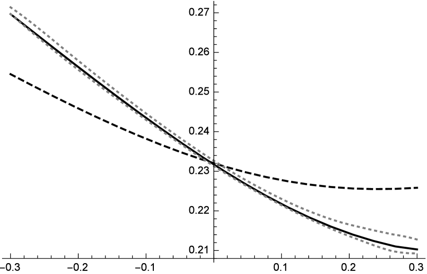
Figure 3: Implied volatility (IV) is plotted as a function of $\log$-strike $k:=\log K$ for the model of Section 5.3. The dashed line corresponds to the IV induced by $u^{(0)}(t,x)$. The solid line corresponds to the IV induced by $u^{(3)}(t,x)$. The dotted lines correspond to the $95\%$ confidence interval of IV resulting form a Monte Carlo simulation. We use parameters given in equation (5.19).

and, using Theorem 3.7, we compute the approximate prices $u^{(0)}(t,x;k)$ and $u^{(3)}(t,x;k)$ of a series of European puts with strike prices $k=\log K\in[-0.3,0.3]$ (we once again add the parameter $k$ to the arguments of $u^{(n)}$ to emphasize the dependence of $u^{(n)}$ on the $\log$ strike price $k$). We also compute the exact price $u$ using Monte Carlo simulation. After converting prices to implied volatilities we plot the results in Figure 3. We observe a nearly exact match between the induced implied volatilities $\text{IV}[u^{(3)}(t,x;k)]$ and $\text{IV}[u(t,x;k)]$.

5.4 Yields and credit spreads in the JDCEV setting

Consider a defaultable bond, written on $S$, that pays one dollar at time $T>t$ if no default occurs prior to maturity (i.e., $S_{T}>0$, $\zeta>T$) and pays zero dollars otherwise. Then the time $t$ value of the bond is given by

$$V_{t} =\mathbb{E}[\mathbb{I}_{\{\zeta>T\}}|X_{t}]=\mathbb{I}_{\{\zeta>t\}}u(t,X_{t};T), u(t,X_{t};T) =\mathbb{E}[e^{-\int_{t}^{T}\gamma(s,X_{s})ds}|X_{t}].$$ (5.20)

We add the parameter $T$ to the arguments of $u$ to indicate dependence of $u$ on the maturity date $T$. Note that $u(t,x;T)$ is both the price of a bond and the conditional survival probability: $\mathbb{Q}(\zeta>T|X_{t}=x,\zeta>t)$. The yield $Y(t,x;T)$ of such a bond, on the set $\{\zeta>t\}$, is defined as

$$Y(t,x;T) :=\frac{-\log u(t,x;T)}{T-t}.$$ (5.21)

The credit spread is defined as the yield minus the risk-free rate of interest. Obviously, in the case of zero interest rates, we have: yield $=$ credit spread.

In Carr and Linetsky (2006), the authors introduce a class of unified credit-equity models known as Jump to Default Constant Elasticity of Variance or JDCEV. Specifically, in the time-homogeneous case, the underlying $S$ is described by (2.1) with

$$a(x) =\frac{1}{2}\delta^{2}e^{2\beta x}, \gamma(x) =b+c\,\delta^{2}e^{2\beta x}, \nu(x,dz) =0,$$ (5.22)

where $\delta>0$, $b\geq 0$, $c\geq 0$. We will restrict our attention to cases in which $\beta<0$. From a financial perspective, this restriction makes sense, as it results in volatility and default intensity increasing as $S\to 0^{+}$, which is consistent with the leverage effect. Note that when $c>0$, the asset $S$ may only go to zero via a jump from a strictly positive value. That is, according to the Feller boundary classification for one-dimensional diffusions (see Borodin and Salminen (2002), p.14), the endpoint $-\infty$ is a natural boundary for the killed diffusion $X$ (i.e., the probability that $X$ reaches $-\infty$ in finite time is zero). The survival probability $u(t,x;T)$ in this setting is computed in Mendoza-Arriaga et al. (2010), equation (8.13). We have

$$u(t,x;T) =\sum_{n=0}^{\infty}\bigg{(}e^{-(b+\omega n)(T-t)}\frac{\Gamma(1+c/|\beta|)\Gamma(n+1/(2|\beta|))}{\Gamma(\nu+1)\Gamma(1/(2|\beta|))n!}$$ (5.23)

$$\qquad\times A^{1/(2|\beta|)}e^{x}\exp\left(-Ae^{-2\beta x}\right){}_{1}F_{1}(1-n+c/|\beta|;\nu+1;Ae^{-2\beta x})\bigg{)}$$ (5.24)

where ${}_{1}F_{1}$ is the Kummer confluent hypergeometric function, $\Gamma(x)$ is a Gamma function and

$$\nu =\frac{1+2c}{2|\beta|}, A =\frac{b}{\delta^{2}|\beta|}, \omega =2|\beta|b.$$ (5.25)

We compute $u(t,x;T)$ using both equation (5.24) (truncating the infinite series at $n=70$) as well as using Theorem 3.7. We use the Taylor series expansion of $\mathscr{A}$ expansion of Example 3.2 with $\bar{x}=X_{t}$. After computing bond prices, we then calculate the corresponding credit spreads using (5.21). Approximate spreads are denoted

$$Y^{(n)}(t,x;T) :=\frac{-\log u^{(n)}(t,x;T)}{T-t}.$$ (5.26)

The survival probabilities are and the corresponding yields are plotted in Figure 4. Values for the yields from Figure 4 can also be found in Table 2.

Remark 5.1.

To compute survival probabilities $u(t,x;T)$, one assumes a payoff function $h(x)=1$ and obtains

$$u(t,x;T)=\int_{\mathbb{R}}p(t,x;T,y)dy=\hat{p}(t,x;T,0).$$

Thus, when computing survival probabilities and/or credit spreads, no numerical integration is required. Rather, one uses (3.25) and easily obtains

$$u_{0}(t,x;T) =e^{-\left(b+\delta^{2}ce^{2x\beta}\right)\tau},$$ (5.27)

$$u_{1}(t,x;T) =e^{-\left(b+\delta^{2}ce^{2x\beta}\right)\tau}\left(-\delta^{2}bce^{2x\beta}\tau^{2}\beta+\frac{1}{2}\delta^{4}ce^{4x\beta}\tau^{2}\beta-\delta^{4}c^{2}e^{4x\beta}\tau^{2}\beta\right),$$ (5.28)

$$u_{2}(t,x;T) =e^{-\left(b+\delta^{2}ce^{2x\beta}\right)\tau}\Big{(}-\delta^{4}ce^{4x\beta}\tau^{2}\beta^{2}-\frac{2}{3}\delta^{2}b^{2}ce^{2x\beta}\tau^{3}\beta^{2}+\delta^{4}bce^{4x\beta}\tau^{3}\beta^{2}$$ (5.29)

$$\qquad-2\delta^{4}bc^{2}e^{4x\beta}\tau^{3}\beta^{2}-\frac{1}{3}\delta^{6}ce^{6x\beta}\tau^{3}\beta^{2}+2\delta^{6}c^{2}e^{6x\beta}\tau^{3}\beta^{2}$$ (5.30)

$$\qquad-\frac{4}{3}\delta^{6}c^{3}e^{6x\beta}\tau^{3}\beta^{2}+\frac{1}{2}\delta^{4}b^{2}c^{2}e^{4x\beta}\tau^{4}\beta^{2}-\frac{1}{2}\delta^{6}bc^{2}e^{6x\beta}\tau^{4}\beta^{2}+\delta^{6}bc^{3}e^{6x\beta}t^{4}\beta^{2}$$ (5.31)

$$\qquad+\frac{1}{8}\delta^{8}c^{2}e^{8x\beta}\tau^{4}\beta^{2}-\frac{1}{2}\delta^{8}c^{3}e^{8x\beta}\tau^{4}\beta^{2}+\frac{1}{2}\delta^{8}c^{4}e^{8x\beta}\tau^{4}\beta^{2}\Big{)}.$$ (5.32)

where $\tau:=T-t$. It is interesting to note that

$$u^{(n)}(t,x;T) =\sum_{k=0}^{n}u_{k}(t,x;T)=e^{-\left(b+\delta^{2}ce^{2x\beta}\right)\tau}\left(1+\mathscr{O}(\tau^{2})\right),$$ (5.33)

which guarantees that the $\partial_{\tau}u^{(n)}|_{\tau=0}<0$ (i.e., as $\tau$ increases from zero, the approximate survival probability decreases, as expected).

5.5 Hermite vs Taylor approximations

We are interested in comparing the relative accuracy of the Taylor series and Hermite polynomial approximations (examples 3.2 and 3.4). To this end, we consider the Constant Elasticity of Variance (CEV) model of Cox (1975). The $\log$ dynamics are given by

$$a(x) =\frac{1}{2}\delta^{2}e^{2(\beta-1)x}, \nu(x,dz) =0, \gamma(x) =0, \beta \in[0,1],$$ (5.34)

We consider two approximations for the variance function $a$ – Taylor and Hermite. We have

$$\text{Taylor}: a_{\text{T}}^{(n)}(x) :=\sum_{k=0}^{n}\frac{\partial_{x}^{k}a(\bar{x})}{k!}(x-\bar{x})^{k},$$ (5.35)

$$\text{Hermite}: a_{\text{H}}^{(n)}(x) :=\sum_{k=0}^{n}\langle a,\mathbf{H}_{k}(\cdot-\bar{x})\rangle_{\Gamma}\mathbf{H}_{k}(x-\bar{x}),$$ (5.36)

Fix a maturity date $T$ and let $t<T$. Denote by $u(t,x;K)$ the price at time $t<T$ of a call option with strike price $K$. The exact call option price is given in Cox (1975). Denote by $u_{\text{T}}^{(n)}(t,x;K)$ the $n$th order approximation of a call price, as obtained using the Taylor series approximation of $a$. Likewise, denote by $u_{\text{H}}^{(n)}(t,x;K)$ the $n$th order approximation of a call price, as obtained using the Hermite polynomial approximation of $a$. In figure 5 we plot as a function of $\log$ moneyness $k:=(\log K-x)$ the exact implied volatility $\text{IV}[u(t,x;K)]$ as well as the Taylor and Hermite approximations of implied volatility $\text{IV}[u_{\text{T}}^{(n)}(t,x;K)]$ and $\text{IV}[u_{\text{H}}^{(n)}(t,x;K)]$ for $n=\{0,1,2,3,4\}$. We also plot, as a function of $x$ the exact diffusion coefficient $a(x)$ as well as the Taylor and Hermite approximations of the diffusion coefficient $a_{\text{T}}^{(n)}(x)$ and $a_{\text{H}}^{(n)}(x)$ for $n=\{0,1,2,3,4\}$. It is clear from Figure 5 that the Taylor expansion $a_{\text{T}}^{(n)}(x)$ provides a more accurate approximation of $a(x)$ than the Hermite expansion $a_{\text{H}}^{(n)}(x)$ for every $n\leq 4$. Not surprisingly, Figure 5 also shows that implied volatility induced by the Taylor expansion $\text{IV}[u_{\text{T}}^{(n)}(t,x;K)]$ provides a more accurate approximation of the exact implied volatility $\text{IV}[u(t,x;K)]$ than does the Hermite approximation $\text{IV}[u_{\text{H}}^{(n)}(t,x;K)]$. Though, for $n=4$, both approximations are remarkably accurate for $\log$ moneyness $k\in(-0.4,0.4)$.

5.6 Accuracy: jumps vs no jumps

In this example, we examine (numerically) whether or not the addition of jumps affects the accuracy of our asymptotic approximation for Call prices. To this end, we consider the CEV-like Lévy-type process with Gaussian jumps, introduced in Section 5.1. We fix the following parameters:

$$\delta =0.20, \beta =0.5, m =-0.1, \eta =0.2, S_{0}=e^{x} =1, T-t =0.5.$$ (5.37)

We consider two scenarios: $\lambda=0$ (no jumps) and $\lambda=0.2$ (with jumps). In each scenario we compute our third order approximation for Call prices $u^{(3)}(t,x;K)$ using the Taylor series approximation (Example 3.2). We also compute, in the case of no jumps, the exact call price using the formulas given in Cox (1975). In the case where the jump intensity $\lambda$ is non-zero, we compute a 95% confidence interval for call prices via Monte Carlo simulation. Finally, call prices are converted to implied volatilities: $\text{IV}[u(t,x;K)]$. The results are plotted in Figure 6.

6 Proof of Theorem 4.4

For sake of simplicity we only prove the assertion when the default intensity and mean jump size are zero ${\gamma}=m=0$, when the jump intensity and diffusion component are time-independent $a(t,x)\equiv a(x)$, $\lambda(t,x)\equiv\lambda(x)$ and when the standard deviation of the jumps is constant $\delta(x)\equiv\delta$. Thus we consider the integro-differential operator

$$Lu(t,x) ={\partial}_{t}u(t,x)+\frac{a(x)}{2}({\partial}_{xx}-{\partial}_{x})u(t,x)-\lambda(x)\left(e^{\frac{\delta^{2}}{2}}-1\right){\partial}_{x}u(t,x)$$

$$\qquad+\lambda(x)\int_{{\mathbb{R}}}\left(u(t,x+z)-u(t,x)\right)\nu_{\delta^{2}}(dz),$$

with

$$\nu_{\delta^{2}}(dz) =\frac{1}{\sqrt{2\pi}\delta}e^{-\frac{z^{2}}{2\delta^{2}}}dz.$$ (6.1)

We will give some details on how to extend the proof to the general case at the end of the section. Our idea is to use our expansion as a parametrix. That is, our expansion will serve as the starting point of the classical iterative method introduced by Levi (1907) to construct the fundamental solution $p(t,x;T,y)$ of $L$. Specifically, as in Pagliarani et al. (2013), we take as a parametrix our $N$-th order approximation $p^{(N)}(t,x;T,y)$ with $\bar{x}=y$ in (4.10)-(4.11). The case $\bar{x}=x$ can be analogously proved by using the backward parametrix approach (see Corielli et al. (2011)). For sake of brevity we skip the details for the latter case.

By analogy with the classical approach (see, for instance, Friedman (1964) and Di Francesco and Pascucci (2005), Pascucci (2011) for the pure diffusive case, or Garroni and Menaldi (1992) for the integro-differential case), we have

$$p(t,x;T,y)=p^{(N)}(t,x;T,y)+\int_{t}^{T}\int_{{\mathbb{R}}}p^{(0)}(t,x;s,{\xi})\Phi(s,{\xi};T,y)d{\xi}ds,$$ (6.2)

where $\Phi$ is determined by imposing the condition

$$0=Lp(t,x;T,y)=Lp^{(N)}(t,x;T,y)+\int_{t}^{T}\int_{{\mathbb{R}}}Lp^{(0)}(t,x;s,{\xi})\Phi(s,{\xi};T,y)d{\xi}ds-\Phi(t,x;T,y).$$

Equivalently, we have

$$\Phi(t,x;T,y)=Lp^{(N)}(t,x;T,y)+\int_{t}^{T}\int_{{\mathbb{R}}}Lp^{(0)}(t,x;s,{\xi})\Phi(s,{\xi};T,y)d{\xi}ds,$$

and therefore by iteration

$$\Phi(t,x;T,y)=\sum_{n=0}^{\infty}Z^{(N)}_{n}(t,x;T,y),$$ (6.3)

where

$$Z^{(N)}_{0}(t,x;T,y) :=Lp^{(N)}(t,x;T,y),$$ (6.4)

$$Z^{(N)}_{n+1}(t,x;T,y) :=\int_{t}^{T}\int_{{\mathbb{R}}}Lp^{(0)}(t,x;s,{\xi})Z^{(N)}_{n}(s,{\xi};T,y)d{\xi}ds.$$ (6.5)

The proof of Theorem 4.4 is based on several technical lemmas which we relegate to Section 6.3. In particular, we will use such preliminary estimates to provide pointwise bounds for each of the terms $Z^{(N)}_{n}$ in (6.3). Finally, these bounds combined with formula (6.2) give the estimate of $\left|p(t,x;T,y)-p^{(N)}(t,x;T,y)\right|$.

For any ${\alpha},\theta>0$ and ${\ell}\geq 0$, consider the integro-differential operators

$$L^{{\alpha},\theta,{\ell}}u(t,x) ={\partial}_{t}u(t,x)+\frac{{\alpha}}{2}({\partial}_{xx}-{\partial}_{x})u(t,x)-{\ell}\left(e^{\frac{\theta}{2}}-1\right){\partial}_{x}u(t,x)+{\ell}\int_{{\mathbb{R}}}\left(u(t,x+z)-u(t,x)\right)\nu_{\theta}(dz),$$ (6.6)

$$\bar{L}^{{\alpha},\theta,{\ell}}u(t,x) ={\partial}_{t}u(t,x)+\frac{{\alpha}}{2}{\partial}_{xx}u(t,x)+{\ell}\int_{{\mathbb{R}}}\left(u(t,x+z)-u(t,x)\right)\nu_{\theta}(dz).$$ (6.7)

The function $\Gamma^{{\alpha},\theta,{\ell}}(t,x;T,y):=\Gamma^{{\alpha},\theta,{\ell}}(T-t,x-y)$ where

$$\Gamma^{{\alpha},\theta,{\ell}}(t,x) :=e^{-{\ell}t}\sum_{n=0}^{\infty}\frac{({\ell}t)^{n}}{n!}\Gamma_{n}^{{\alpha},\theta,{\ell}}(t,x),$$ (6.8)

$$\Gamma_{n}^{{\alpha},\theta,{\ell}}(t,x) :=\frac{1}{\sqrt{2\pi({\alpha}t+n\theta)}}\exp\left(-\frac{\left(x-\left(\frac{{\alpha}}{2}+{\ell}e^{\frac{\theta}{2}}-{\ell}\right)t\right)^{2}}{2({\alpha}t+n\theta)}\right),$$ (6.9)

is the fundamental solution of $L^{{\alpha},\theta,{\ell}}$. Analogously, the function $\bar{\Gamma}^{{\alpha},\theta,{\ell}}(t,x;T,y):=\bar{\Gamma}^{{\alpha},\theta,{\ell}}(T-t,x-y)$ where

$$\bar{\Gamma}^{{\alpha},\theta,{\ell}}(t,x) :=e^{-{\ell}t}\sum_{n=0}^{\infty}\frac{({\ell}t)^{n}}{n!}\bar{\Gamma}_{n}^{{\alpha},\theta}(t,x),$$ (6.10)

$$\bar{\Gamma}_{n}^{{\alpha},\theta}(t,x) :=\frac{1}{\sqrt{2\pi({\alpha}t+n\theta)}}\exp\left(-\frac{x^{2}}{2({\alpha}t+n\theta)}\right),$$ (6.11)

is the fundamental solution of $\bar{L}^{{\alpha},\theta,{\ell}}$. Note that under our assumptions, at order zero, by (4.4)-(4.5) we have

$$p^{(0)}(t,x;T,y)=\Gamma^{a\left(y\right),\delta^{2},\lambda(y)}(t,x;T,y).$$ (6.12)

We also recall the definition of convolution operator $\mathscr{C}_{\theta}$:

$$\mathscr{C}_{\theta}f(x)=\mathscr{C}^{x}_{0,\theta}f(x):=\int_{{\mathbb{R}}}f(x+z)\frac{1}{\sqrt{2\pi\theta}}e^{-\frac{z^{2}}{2\theta}}dz.$$ (6.13)

Note that, for any $\theta>0$, we have

$$\mathscr{C}_{\theta}\Gamma^{{\alpha},\theta,{\ell}}(t,\cdot)(x) =e^{-{\ell}t}\sum_{n=0}^{\infty}\frac{({\ell}t)^{n}}{n!}\Gamma_{n+1}^{{\alpha},\theta,{\ell}}(t,x),$$ (6.14)

$$\mathscr{C}_{\theta}\bar{\Gamma}^{{\alpha},\theta,{\ell}}(t,\cdot)(x) =e^{-{\ell}t}\sum_{n=0}^{\infty}\frac{({\ell}t)^{n}}{n!}\bar{\Gamma}_{n+1}^{{\alpha},\theta}(t,x),$$ (6.15)

with $\bar{\Gamma}_{n}^{{\alpha},\theta}$ and $\Gamma_{n}^{{\alpha},\theta,{\ell}}$ as in (6.9) and (6.11) respectively.

Proposition 6.1.

For any $c>1$ and ${\tau}>0$, there exists a positive constant $C$, only dependent on $c,{\tau},M,N$, and $(\|a_{i}\|_{\infty},\|\lambda_{i}\|_{\infty})_{i=1,\cdots,N+1}$, such that

$$\big{|}Z^{(N)}_{n}(t,x;T,y)\big{|}\leq\frac{C^{n+1}{(T-t)^{\frac{\min{(1,N)}+n-1}{2}}}}{\sqrt{n!}}\left(1+\|\lambda_{1}\|_{\infty}\mathscr{C}_{cM}^{n+1}\right)\,\bar{\Gamma}^{cM,cM,cM}(t,x;T,y),$$ (6.16)

for any $n\in\mathbb{N}_{0}$, $x,y\in{\mathbb{R}}$ and $t,T\in{\mathbb{R}}$ with $0<T-t\leq{\tau}$.

The proof of Proposition 6.1 is postponed to Section 6.1. We are now in position to prove Theorem 4.4. Indeed, by equations (6.2), (6.3) and Proposition 6.1 we have

$$\big{|}p(t,x;T,y)-p^{(N)}(t,x;T,y)\big{|}$$

$$\leq\sum_{n=0}^{\infty}\frac{C^{n+1}}{\sqrt{n!}}\int_{t}^{T}{(T-s)^{\frac{\min{(1,N)}+n-1}{2}}}\int_{{\mathbb{R}}}p^{(0)}(t,x;s,{\xi})\ \left(1+\|\lambda_{1}\|_{\infty}\mathscr{C}_{cM}^{n+1}\right)\bar{\Gamma}^{cM,cM,cM}(s,{\xi};T,y)d{\xi}ds$$

(and by Lemma 6.4 with $$\eta=0$$)

$$\leq\sum_{n=0}^{\infty}\frac{C^{n+1}}{\sqrt{n!}}\int_{t}^{T}{(T-s)^{\frac{\min{(1,N)}+n-1}{2}}}\int_{{\mathbb{R}}}\bar{\Gamma}^{cM,cM,cM}(t,x;s,{\xi})\ \left(1+\|\lambda_{1}\|_{\infty}\mathscr{C}_{cM}^{n+1}\right)\bar{\Gamma}^{cM,cM,cM}(s,{\xi};T,y)d{\xi}ds$$ .

Now, by the semigroup property

$$\int_{{\mathbb{R}}}\mathscr{C}_{\theta}^{k}\bar{\Gamma}^{\alpha,\theta,{\ell}}(t,x;s,{\xi})\mathscr{C}_{\theta}^{N}\bar{\Gamma}^{\alpha,\theta,{\ell}}(s,{\xi};T,y)\,d{\xi}=\mathscr{C}_{\theta}^{k+N}\bar{\Gamma}^{\alpha,\theta,{\ell}}(t,x;T,y),\qquad k,N\in\mathbb{N}_{0},$$ (6.17)

we get

$$\big{|}p(t,x;T,y)-p^{(N)}(t,x;T,y)\big{|} \leq 2\,{(T-s)^{\frac{\min{(1,N)}+1}{2}}}\left(\sum_{n=0}^{\infty}\frac{C^{n+1}(T-t)^{\frac{n}{2}}}{\sqrt{n!}}\left(1+\|\lambda_{1}\|_{\infty}\mathscr{C}_{cM}^{n+1}\right)\bar{\Gamma}^{cM,cM,cM}(t,x;T,y)\right),$$

for any $x,y\in{\mathbb{R}}$ and $t,T\in{\mathbb{R}}$ with $0<T-t\leq{\tau}$, and since

$$\sum_{n=0}^{\infty}\frac{C^{n+1}(T-t)^{\frac{n}{2}}}{\sqrt{n!}}\,\mathscr{C}_{cM}^{n+1}\bar{\Gamma}^{cM,cM,cM}(t,x;T,y)$$

can be easily checked to be convergent, this concludes the proof of Theorem 4.4.

We conclude this section with a brief discussion on how to drop the additional hypothesis on the coefficients introduced at the beginning of the section. In order to include state-dependency in the standard deviation of the jumps, i.e. $\delta=\delta(x)$, no modification is required in the first part of the proof since all the preliminary lemmas in Section 6.3 naturally apply to the general case. On the other hand, the proof of Proposition 6.1 requires some simple modifications to account for the additional terms in the expansion introduced by the state dependency of the convolution operator (see Proposition 4.1). To extend the proof to non-null mean of the jumps, i.e. $m=m(x)\neq 0$, it is enough to extend Lemmas 6.4-6.10 to the more general functions such as

$$\Gamma^{{\alpha},m,\theta,{\ell}}(t,x) :=e^{-{\ell}t}\sum_{n=0}^{\infty}\frac{({\ell}t)^{n}}{n!}\Gamma_{n}^{{\alpha},m,\theta,{\ell}}(t,x),$$ (6.18)

$$\Gamma_{n}^{{\alpha},m,\theta,{\ell}}(t,x) :=\frac{1}{\sqrt{2\pi({\alpha}t+n\theta)}}\exp\left(-\frac{\left(x+nm-\left(\frac{{\alpha}}{2}+{\ell}e^{\frac{\theta}{2}}-{\ell}\right)t\right)^{2}}{2({\alpha}t+n\theta)}\right).$$ (6.19)

As for the time-dependency of the coefficients $a(t,x)$ and $\gamma(t,x)$, the proof easily follows by the regularity hypothesis iii) in Assumption 4.3.

6.1 Proof of Proposition 6.1

The proof of Proposition 6.1 is based on the two following propositions.

Proposition 6.2.

For any $c>1$ and ${\tau}>0$, there exists a positive constant $C$, only dependent on $c,{\tau},M,\|\lambda_{1}\|_{\infty}$ and $\|a_{1}\|_{\infty}$, such that

$$\left|(x-y)^{2-n}(\partial_{xx}-\partial_{x})p_{n}(t,x;T,y)\right|\leq C(1+\|\lambda_{1}\|_{\infty}\mathscr{C}_{cM})\ \bar{\Gamma}^{cM,cM,cM}(t,x;T,y),$$ (6.20)

for any $n\in\{0,1\}$, $x,y\in{\mathbb{R}}$ and $t,T\in{\mathbb{R}}$ with $0<T-t\leq{\tau}$.

Proof.

Recalling the expression of $p_{0}(t,x;T,y)\equiv p^{(0)}(t,x;T,y)$ in (6.12), the case $n=0$ directly follows from Lemmas 6.5, 6.8 and 6.4 with $\eta=0$.

For the case $n=1$ we first observe that, by Theorem 3.7 along with Proposition 4.1, the function $p_{1}(t,x;T,y)$ takes the form

$$p_{1}(t,x;T,y)=\left((T-t)(x-y)+\frac{(T-t)^{2}}{2}J\right)\mathscr{A}_{1}p^{(0)}(t,x;T,y),$$ (6.21)

where $J$ is the operator

$$J=a_{0}(2\partial_{x}-1)-\lambda_{0}\left(e^{\frac{\delta^{2}}{2}}-1+\delta^{2}\partial_{x}\mathscr{C}_{\delta^{2}}\right),$$ (6.22)

whereas $\mathscr{A}_{1}$ acts as

$$\mathscr{A}_{1} =a_{1}(\partial_{xx}-\partial_{x})-\lambda_{1}\left(\left(e^{\frac{\delta^{2}}{2}}-1\right)\partial_{x}-\mathscr{C}_{\delta^{2}}+1\right),$$ (6.23)

and $\mathscr{C}_{\delta^{2}}$ is the convolution operator defined in (6.13). Therefore, we have

$$(x-y)(\partial_{xx}-\partial_{x})v_{1}(t,x;T,y) =(T-t)(x-y)\left((x-y)(\partial_{xx}-\partial_{x})+2\partial_{x}-1\right)\mathscr{A}_{1}p^{(0)}(t,x;T,y)$$

$$\quad+\frac{(T-t)^{2}}{2}(x-y)J(\partial_{xx}-\partial_{x})\mathscr{A}_{1}p^{(0)}(t,x;T,y),$$

In the computations that follow below, in order to shorten notation, we omit the dependence of $t,x,T,y$ in any function. By the commutative property of the operators $\partial_{x}$ and $\mathscr{C}$, and by applying Lemmas 6.5, 6.6 and 6.8 with $\eta=1$, there exists a positive constant $C_{1}$ only dependent on $c,{\tau},M,\|\lambda_{1}\|_{\infty}$ and $\|a_{1}\|_{\infty}$ such that

$$|(T-t)(x-y)\left((x-y)(\partial_{xx}-\partial_{x})+2\partial_{x}-1\right)a_{1}(\partial_{xx}-\partial_{x})p^{(0)}| \leq C_{1}\Gamma^{ca(y),c\delta^{2},\lambda(y)},$$ (6.24)

$$\left|(T-t)(x-y)\left((x-y)(\partial_{xx}-\partial_{x})+2\partial_{x}-1\right)\lambda_{1}\left(\left(e^{\frac{\delta^{2}}{2}}-1\right)\partial_{x}+1\right)p^{(0)}\right| \leq C_{1}\left(\Gamma^{ca(y),c\delta^{2},\lambda(y)}+\Gamma^{ca(y),4c\delta^{2},\lambda(y)}\right),$$ (6.25)

$$\frac{(T-t)^{2}}{2}|(x-y)J(\partial_{xx}-\partial_{x})a_{1}(\partial_{xx}-\partial_{x})p^{(0)}| \leq C_{1}\left(\Gamma^{ca(y),c\delta^{2},\lambda(y)}+\Gamma^{ca(y),4c\delta^{2},\lambda(y)}\right),$$ (6.26)

$$\frac{(T-t)^{2}}{2}\left|(x-y)J(\partial_{xx}-\partial_{x})\lambda_{1}\left(\left(e^{\frac{\delta^{2}}{2}}-1\right)\partial_{x}+1\right)p^{(0)}\right| \leq C_{1}\left(\Gamma^{ca(y),c\delta^{2},\lambda(y)}+\Gamma^{ca(y),4c\delta^{2},\lambda(y)}\right),$$ (6.27)

for any $x,y\in{\mathbb{R}}$ and $t,T\in{\mathbb{R}}$ with $0<T-t\leq{\tau}$. Analogously, by the commutative property of $\partial_{x}$ and $\mathscr{C}$, and by applying Lemmas 6.8, 6.5, 6.9 and 6.7 with $\eta=2$, there exists a positive constant $C_{2}$ only dependent on $c,{\tau},M,\|\lambda_{1}\|_{\infty}$ and $\|a_{1}\|_{\infty}$ such that

$$|(T-t)(x-y)\left((x-y)(\partial_{xx}-\partial_{x})+2\partial_{x}-1\right)\lambda_{1}\mathscr{C}_{\delta^{2}}p^{(0)}| \|\lambda_{1}\|_{\infty}\leq C_{2}\,\left(\mathscr{C}_{c\delta^{2}}\Gamma^{ca(y),c\delta^{2},\lambda(y)}+\mathscr{C}_{4c\delta^{2}}\Gamma^{ca(y),4c\delta^{2},\lambda(y)}\right),$$ (6.28)

$$\frac{(T-t)^{2}}{2}|(x-y)J(\partial_{xx}-\partial_{x})\lambda_{1}\mathscr{C}_{\delta^{2}}p^{(0)}| \leq\|\lambda_{1}\|_{\infty}\,C_{2}\left(\mathscr{C}_{c\delta^{2}}\Gamma^{ca(y),c\delta^{2},\lambda(y)}+\mathscr{C}_{4c\delta^{2}}\Gamma^{ca(y),4c\delta^{2},\lambda(y)}\right),$$ (6.29)

for any $x,y\in{\mathbb{R}}$ and $t,T\in{\mathbb{R}}$ with $0<T-t\leq{\tau}$. Then, (6.20) follows from (6.27) and (6.29) by applying Lemma 6.4 with $\eta=0$ and $\eta=1$ respectively. ∎

Proposition 6.3.

For any $c>1$ and ${\tau}>0$, there exists a positive constant $C$, only dependent on $c,{\tau},M,\|\lambda_{1}\|_{\infty}$ and $\|a_{1}\|_{\infty}$, such that

$$\left|(x-y)^{2-n}\left(\left(e^{\frac{\delta^{2}}{2}}-1\right)\partial_{x}+\mathscr{C}_{\delta^{2}}-1\right)p_{n}(t,x;T,y)\right|\leq C(1+\mathscr{C}_{cM})\,\bar{\Gamma}^{cM,cM,cM}(t,x;T,y),$$ (6.30)

for any $n\in\{0,1\}$, $x,y\in{\mathbb{R}}$ and $t,T\in{\mathbb{R}}$ with $0<T-t\leq{\tau}$.

Proof.

For simplicity we only prove the thesis for $n=0$. The proof for $n=1$ is entirely analogous to that of Proposition 6.2. Once again, hereafter we omit the dependence of $t,x,T,y$ in any function we consider. Recalling the expression of $p_{0}(t,x;T,y)\equiv p^{(0)}(t,x;T,y)$ in (6.12), by Lemmas 6.5, 6.8 and 6.9, there exists a positive constant $C_{1}$ only dependent on $c,{\tau},M$ such that

$$\left|(x-y)^{2}\left(\left(e^{\frac{\delta^{2}}{2}}-1\right)\partial_{x}+\mathscr{C}_{\delta^{2}}-1\right)v_{0}\right|\leq C_{1}\left(\Gamma^{ca(y),4c\delta^{2},\lambda(y)}+(1+\mathscr{C}_{16c\delta^{2}})\Gamma^{ca(y),16c\delta^{2},\lambda(y)}\right),$$

for any $x,y\in{\mathbb{R}}$ and $t,T\in{\mathbb{R}}$ with $0<T-t\leq{\tau}$. Then, (6.30) follows from Lemma 6.4 with $\eta=0$ and with $\eta=1$. ∎

We are now in position to prove Proposition 6.1.

Proof of Proposition 6.1.

We first prove the case $N=1$. Let us define the operators

$$L_{0}=\partial_{t}+\mathscr{A}_{0},\qquad L_{1}=\partial_{t}+\mathscr{A}_{0}+(x-y)\mathscr{A}_{1}.$$

Let us recall that, by (3.12) and (3.13) with $n=1$, we have

$$L_{0}p_{0}=0,\qquad L_{0}p_{1}=-(L_{1}-L_{0})p_{0}.$$

Thus, by (6.4) we have

$$Z^{(1)}_{0}(t,x;T,y)=Lp^{(1)}(t,x;T,y) =Lp_{0}(t,x;T,y)+Lp_{1}(t,x;T,y)$$

$$=(L-L_{1})p_{0}(t,x;T,y)+(L-L_{0})p_{1}(t,x;T,y),$$

where $(L-L_{0})$ and $(L-L_{1})$ are explicitly given by

$$(L-L_{0}) =(a(x)-a(y))(\partial_{xx}-\partial_{x})+(\lambda(x)-\lambda(y))\left(\left(e^{\frac{\delta^{2}}{2}}-1\right)\partial_{x}+\mathscr{C}_{\delta^{2}}-1\right),$$ (6.31)

$$(L-L_{1}) =(a(x)-a(y)-a^{\prime}(y)(x-y))(\partial_{xx}-\partial_{x})$$ (6.32)

$$\quad+(\lambda(x)-\lambda(y)-\lambda^{\prime}(y)(x-y))\left(\left(e^{\frac{\delta^{2}}{2}}-1\right)\partial_{x}+\mathscr{C}_{\delta^{2}}-1\right).$$ (6.33)

Thus, by the Lipschitz assumptions on $a$, $\lambda$ and their first order derivatives, we obtain

$$|Z^{(1)}_{0}(t,x;T,y)| \leq\|a_{2}\|_{\infty}|x-y|^{2}|(\partial_{xx}-\partial_{x})p_{0}(t,x;T,y)|+\|a_{1}\|_{\infty}|x-y||(\partial_{xx}-\partial_{x})p_{1}(t,x;T,y)|$$ (6.34)

$$\qquad\ +\|\lambda_{2}\|_{\infty}|x-y|^{2}\left|\left(\left(e^{\frac{\delta^{2}}{2}}-1\right)\partial_{x}+\mathscr{C}_{\delta^{2}}-1\right)p_{0}(t,x;T,y)\right|$$ (6.35)

$$\qquad\ +\|\lambda_{1}\|_{\infty}|x-y|\left|\left(\left(e^{\frac{\delta^{2}}{2}}-1\right)\partial_{x}+\mathscr{C}_{\delta^{2}}-1\right)p_{1}(t,x;T,y)\right|.$$ (6.36)

and, as $\|\lambda_{1}\|_{\infty}=0$ implies $\|\lambda_{2}\|_{\infty}=0$, by Propositions 6.2 and 6.3 there exists a positive constant $C$, only dependent on $c,{\tau},M$,$\|\lambda_{1}\|_{\infty}$,$\|\lambda_{2}\|_{\infty}$, $\|a_{1}\|_{\infty}$ and $\|a_{2}\|_{\infty}$, such that (6.16) holds for $N=1$ and $n=0$. To prove the general case, we proceed by induction on $n$. First note that, by (3.12) we have

$$|Lp^{(0)}(t,x;T,y)| =|(L-L_{0})p^{(0)}(t,x;T,y)|$$ (6.37)

(and by (6.31) and the Lipschitz property of $${\alpha},\lambda$$)

$$\leq\|a_{1}\|_{\infty}|x-y||(\partial_{xx}-\partial_{x})p^{(0)}(t,x;T,y)|$$ (6.38)

$$\quad\ +\|\lambda_{1}\|_{\infty}|x-y|\left|\left(\left(e^{\frac{\delta^{2}}{2}}-1\right)\partial_{x}+\mathscr{C}_{\delta^{2}}-1\right)p^{(0)}(t,x;T,y)\right|$$ (6.39)

(and by applying Lemmas 6.4, 6.5, 6.8 and 6.9 with $$\eta=0,1$$)

$$\leq C_{0}\left(\frac{1}{\sqrt{T-t}}+\|\lambda_{1}\|_{\infty}\mathscr{C}_{cM}\right)\bar{\Gamma}^{cM,cM,cM}(t,x;T,y),$$ (6.40)

for any $x,y\in{\mathbb{R}}$ and $t,T\in{\mathbb{R}}$ with $0<T-t\leq{\tau}$, and where $C_{0}$ is a positive constant only dependent on $c,{\tau},M,\|\lambda_{1}\|_{\infty}$ and $\|a_{1}\|_{\infty}$. Assume now (6.16) holds for $n\geq 0$. Then by (6.5) we obtain

$$|Z^{(1)}_{n+1}(t,x;T,y)| \leq\int_{t}^{T}\int_{{\mathbb{R}}}|Lp^{(0)}(t,x;s,{\xi})||Z^{(1)}_{n}(s,{\xi};T,y)|d{\xi}ds$$ (6.41)

(and by inductive hypothesis and by (6.40))

$$\leq\frac{C^{n+1}C_{0}}{\sqrt{n!}}\int_{t}^{T}(T-s)^{\frac{n}{2}}\int_{{\mathbb{R}}}\left(\frac{1}{\sqrt{s-t}}+\|\lambda_{1}\|_{\infty}\mathscr{C}_{cM}\right)\bar{\Gamma}^{cM,cM,cM}(t,x;s,{\xi})$$ (6.42)

$$\quad\cdot\left(1+\|\lambda_{1}\|_{\infty}\mathscr{C}_{cM}^{n+1}\right)\bar{\Gamma}^{cM,cM,cM}(s,{\xi};T,y)d{\xi}ds.$$ (6.43)

Now, by the semigroup property (6.17), and by the fact that

$$\int_{t}^{T}\frac{(T-s)^{\frac{n}{2}}}{\sqrt{s-t}}ds=\frac{\sqrt{\pi}(T-t)^{\frac{n+1}{2}}\Gamma_{E}\left(\frac{2+n}{2}\right)}{\Gamma_{E}\left(\frac{3+n}{2}\right)}\leq\frac{{\kappa}(T-t)^{\frac{n+1}{2}}}{\sqrt{n+1}},$$ (6.44)

with ${\kappa}=\sqrt{2}\pi$, we obtain

$$|Z^{(1)}_{n+1}(t,x;T,y)| \leq\frac{C^{n+1}C_{0}}{\sqrt{n!}}\left(\frac{{\kappa}(T-t)^{\frac{n+1}{2}}}{\sqrt{n+1}}\left(1+\|\lambda_{1}\|_{\infty}\mathscr{C}_{cM}^{n+1}\right)\right)\bar{\Gamma}^{cM,cM,cM}(t,x;T,y)$$ (6.45)

$$\quad+\frac{C^{n+1}C_{0}}{\sqrt{n!}}\left(\frac{2(T-t)^{\frac{n+2}{2}}}{n+2}\|\lambda_{1}\|_{\infty}\left(\mathscr{C}_{cM}+\|\lambda_{1}\|_{\infty}\mathscr{C}_{cM}^{n+2}\right)\right)\bar{\Gamma}^{cM,cM,cM}(t,x;T,y).$$ (6.46)

Now, by Lemma 6.10 we have

$$\mathscr{C}_{cM}^{n+1}\bar{\Gamma}^{cM,cM,cM}(t,x;T,y) \leq 2\,\mathscr{C}_{cM}^{n+2}\bar{\Gamma}^{cM,cM,cM}(t,x;T,y),$$ (6.47)

$$\mathscr{C}_{cM}\bar{\Gamma}^{cM,cM,cM}(t,x;T,y) \leq\sqrt{n+2}\,\mathscr{C}_{cM}^{n+2}\bar{\Gamma}^{cM,cM,cM}(t,x;T,y).$$ (6.48)

Inserting the above results into (6.46) we obtain

$$|Z^{(1)}_{n+1}(t,x;T,y)| \leq\frac{C^{n+1}C_{0}}{\sqrt{n!}}\frac{(T-t)^{\frac{n+1}{2}}}{\sqrt{n+1}}\left({\kappa}+2\|\lambda_{1}\|_{\infty}\left({\kappa}+\sqrt{{\tau}}(1+\|\lambda_{1}\|_{\infty})\right)\mathscr{C}_{cM}^{n+2}\right)\bar{\Gamma}^{cM,cM,cM}(t,x;T,y)$$ (6.49)

$$\leq\frac{C^{n+1}C_{1}(T-t)^{\frac{n+1}{2}}}{\sqrt{(n+1)!}}\left(1+\|\lambda_{1}\|_{\infty}\mathscr{C}_{cM}^{n+2}\right)\bar{\Gamma}^{cM,cM,cM}(t,x;T,y),$$ (6.50)

where

$$C_{1}=2C_{0}\left({\kappa}+\sqrt{{\tau}}(1+\|\lambda_{1}\|_{\infty})\right).$$ (6.51)

Now, without loss of generality we can assume $C_{1}\leq C$, and thus we obtain (6.16) for $n+1$.

The proof for $N>1$ is based on the same arguments. However, in the general case the technical details become significantly more complicated. In practice, proceeding by induction, one can extend Propositions 6.2 and Proposition 6.3 to a general $n\in{\mathbb{N}}$. Eventually, after proving the identity

$$Lp^{(N)}(t,x;T,y)=\sum_{n=0}^{N}(L-L_{n})p_{N-n}(t,x;T,y),$$ (6.52)

one will be able to prove the estimate (6.16) on $\big{|}Z^{(N)}_{n}(t,x;T,y)\big{|}$ for a generic $N\geq 1$. Finally, the case $N=0$ is simpler because the identity (6.52) simply reduces to

$$Lp^{(0)}(t,x;T,y)=(L-L_{0})p_{0}(t,x;T,y),$$ (6.53)

and the proof becomes a simple application of Lemmas 6.4-6.10. ∎

6.2 Discussion on the difference with respect to the diffusion case

It has been proved by Pagliarani et al. (2013) that, in the purely diffusive case (i.e $\lambda\equiv 0$), error bounds analogous to (4.19) hold with

$$g_{N}(s)=\mathscr{O}\left(s^{\frac{N+1}{2}}\right),\quad\textrm{as }s\to 0^{+}.$$

In other words, the rate of convergence of the $N$-th order approximation as $t\to T^{-}$ is proportional to $(T-t)^{\frac{N+1}{2}}$. The expansion $\sum_{n}p_{n}(t,x;T,y)$ is thus asymptotically convergent in $T-t$. On the other hand, Theorem 4.4 shows that, when considering non-null Lévy measures, the rate of convergence do not improve for $N$ greater than $1$.

The reasons for this discrepancy can be found in the different asymptotic behaviors of the leading term $p_{0}(t,x;T,y)=\Gamma^{a\left(y\right),\delta^{2},\lambda(y)}(t,x;T,y)$ in the fundamental solution expansion of $L$, with and without jumps. Indeed, while the short-time asymptotic behavior at the pole $x=y$ does not change whether $\lambda\equiv 0$ or not, namely $p_{0}(t,x;T,x)\sim\frac{1}{\sqrt{T-t}}$ as $T-t$ goes to $0$, the asymptotic behavior away from the pole radically changes when passing from the purely diffusion to the jump-diffusion case. In particular, by (6.8)-(6.9)-(6.12) it is clear that in general $p_{0}(t,x;T,y)\sim T-t$ as $T-t$ goes to $0$. On the other hand, in the particular case of $L$ being strictly differential, i.e. $\lambda\equiv 0$, the leading term reduces to

$$p_{0}(t,x;T,y)=\Gamma^{a\left(y\right),0,0}(t,x;T,y)=\Gamma_{0}^{a\left(y\right),0,0}(t,x;T,y),$$

which is the Gaussian fundamental solution of a heat-type operator, and thus tends to $0$ exponentially as $T-t$ goes to $0$. For this reason, the differential version of Lemma 6.9 becomes

$$|x-y|\Gamma^{a\left(y\right),0,0}(t,x;T,y)\leq C\sqrt{T-t}\,\Gamma^{ca\left(y\right),0,0}(t,x;T,y),$$ (6.54)

as it is also clear by Lemma 6.8 with $n=0$. Due to this fact, in the purely diffusive case, higher order polynomials of the kind $(x-y)^{N+1}$ arising from the $N$-th order Taylor expansion of the operator $L$, allow to gain an accuracy factor equal to $(T-t)^{\frac{N+1}{2}}$. On the contrary, in the jump-diffusion case, such polynomials can be only used to cancel out the negative powers of the time introduced by the space derivatives, by combining Lemma 6.5 and Lemma 6.8.

6.3 Pointwise estimates

In the rest of the section, we will always assume that

$$M^{-1}\leq{\alpha},\theta\leq M,\qquad 0\leq{\ell}\leq M.$$ (6.55)

Even if not explicitly stated, all the constants appearing in the estimates (6.56), (6.57), (6.59), (6.63), (6.66) and (6.70) of the following lemmas will depend also on $M$.

Lemma 6.4.

For any $T>0$ and $c>1$ there exists a positive constant $C$ such that

$$\mathscr{C}_{\theta}^{\eta}\Gamma^{{\alpha},\theta,{\ell}}(t,x)\leq C\,\mathscr{C}_{cM}^{\eta}\bar{\Gamma}^{cM,cM,cM}(t,x),$$ (6.56)

for any $t\in(0,T]$, $x\in{\mathbb{R}}$ and $\eta\in\mathbb{N}_{0}$.

Proof.

For any $n\geq 0$ we have

$$\Gamma_{n}^{{\alpha},\theta,{\ell}}(t,x)\leq\sqrt{c}Mq_{n}(t,x)\bar{\Gamma}_{n}^{cM,cM}(t,x),$$

where

$$q_{n}(t,x)=\exp\left(-\frac{\left(x-\left(\frac{{\alpha}}{2}+{\ell}e^{\frac{\theta}{2}}-{\ell}\right)t\right)^{2}}{2({\alpha}t+n\theta)}+\frac{x^{2}}{2cM(t+n)}\right).$$

A direct computation shows that

$$\max_{x\in{\mathbb{R}}}q_{n}(t,x) =\exp\left(\frac{s^{2}\left(\alpha+2\left(e^{\frac{\theta}{2}}-1\right){\ell}\right)^{2}}{8\left(cM(n+s)-s\alpha-n\delta^{2}\right)}\right)\leq\exp\left(\frac{T\left(\alpha+2\left(e^{\frac{{\theta}}{2}}-1\right){\ell}\right)^{2}}{8(cM-{\alpha})}\right),$$

for any $t\in(0,T]$, $n\geq 0$ and ${\alpha},\theta,{\ell}$ in (6.55). Then the thesis is a straightforward consequence of the fact that $q_{n}(t,x)$ is bounded on $(0,T]\times{\mathbb{R}}$, uniformly with respect to $n\geq 0$ and ${\alpha},\theta,{\ell}$ in (6.55). ∎

Lemma 6.5.

For any $T>0$, $k\in{\mathbb{N}}$ and $c>1$, there exists a positive constant $C$ such that

$$\left|\partial_{x}^{k}\Gamma_{n}^{{\alpha},\theta,{\ell}}(t,x)\right|\leq\frac{C}{({\alpha}t+n\theta)^{k/2}}\Gamma_{n}^{c{\alpha},c\theta,{\ell}}(t,x),$$ (6.57)

for any $x\in{\mathbb{R}}$, $t\in]0,T]$ and $n\in{\mathbb{N}}_{0}$.

Proof.

For any $k\geq 1$ we have

$$\partial_{x}^{k}\Gamma_{n}^{{\alpha},\theta,{\ell}}(t,x)=\frac{1}{({\alpha}t+n\theta)^{k/2}}\Gamma_{n}^{{\alpha},\theta,{\ell}}(t,x)p_{k}\left(\frac{x-\left(\frac{{\alpha}}{2}+{\ell}e^{\frac{\theta}{2}}-{\ell}\right)t}{\sqrt{{\alpha}t+n\theta}}\right),$$

where $p_{k}$ is a polynomial of degree $k$. To prove the Lemma we will show that there exists a positive constant $C$, which depends only on $m,M,T,c$ and $k$, such that

$$\left(\frac{\left|x-\left(\frac{{\alpha}}{2}+{\ell}e^{\frac{\theta}{2}}-{\ell}\right)t\right|}{\sqrt{{\alpha}t+n\theta}}\right)^{j}\Gamma_{n}^{{\alpha},\theta,{\ell}}(t,x) \leq C\,\Gamma_{n}^{c{\alpha},c\theta,{\ell}}(t,x),\qquad j\leq k.$$ (6.58)

Proceeding as above, we set

$$\left(\frac{\left|x-\left(\frac{{\alpha}}{2}+{\ell}e^{\frac{\theta}{2}}-{\ell}\right)t\right|}{\sqrt{{\alpha}t+n\theta}}\right)^{j}\Gamma_{n}^{{\alpha},\theta,{\ell}}(t,x)=\Gamma_{n}^{c{\alpha},c\theta,{\ell}}(t,x)q_{n,j}(t,x),$$

where

$$q_{n,j}(t,x)=\left(\frac{\left|x-\left(\frac{{\alpha}}{2}+{\ell}e^{\frac{\theta}{2}}-{\ell}\right)t\right|}{\sqrt{{\alpha}t+n\theta}}\right)^{j}\exp\left(-\frac{\left(x-\left(\frac{{\alpha}}{2}+{\ell}e^{\frac{\theta}{2}}-{\ell}\right)t\right)^{2}}{2({\alpha}t+n\theta)}+\frac{\left(x-\left(\frac{c{\alpha}}{2}+{\ell}e^{\frac{c\theta}{2}}-{\ell}\right)t\right)^{2}}{2(c{\alpha}t+nc\theta)}\right).$$

Then the thesis follows from the boundedness of $q_{n,j}$ on $(0,T]\times{\mathbb{R}}$, uniformly with respect to $n\geq 0$ and ${\alpha},\theta,{\ell}$ in (6.55). Indeed the maximum of $q_{n,j}$ can be computed explicitly and we have

$$\lim_{n\to\infty}\left(\max_{x\in{\mathbb{R}},\ t\in]0,T]}q_{n,j}(t,x)\right)=\left(\frac{cj}{(c-1)e}\right)^{\frac{j}{2}}.$$

∎

Lemma 6.6.

For any $T>0$ and $\eta\in{\mathbb{N}}$, there exists a positive constant $C$ such that

$${\ell}t\,\mathscr{C}_{\theta}^{\eta}\Gamma^{{\alpha},\theta,{\ell}}(t,x)\leq C\,\Gamma^{{\alpha},2(\eta+1)\theta,{\ell}}(t,x)$$ (6.59)

for any $t\in(0,T]$ and $x\in{\mathbb{R}}$.

Proof.

We first prove there exists a constant $C_{0}$, which depends only on $m,M,T$ and $\eta$, such that

$$\Gamma_{n+\eta}^{{\alpha},\theta,{\ell}}(t,x) \leq C_{0}\,\Gamma_{n}^{{\alpha},2(\eta+1)\theta,{\ell}}(t,x),$$ (6.61)

$$\Gamma_{\eta}^{{\alpha},\theta,{\ell}}(t,x) \leq C_{0}\,\Gamma_{1}^{{\alpha},2(\eta+1)\theta,{\ell}}(t,x),$$ (6.62)

for any $t\in]0,T]$, $x\in{\mathbb{R}}$, $n\geq 1$ and ${\alpha},\theta,{\ell}$ in (6.55). To prove (6.61) we observe that

$$\Gamma_{n+\eta}^{{\alpha},\theta,{\ell}}(t,x)\leq\frac{1}{\sqrt{2\pi({\alpha}t+(n+\eta)\theta)}}\exp\left(-\frac{\left(x-\left(\frac{{\alpha}}{2}+{\ell}e^{(\eta+1)\theta}-{\ell}\right)t\right)^{2}}{2({\alpha}t+2n(\eta+1)\theta)}\right)q_{n}(t,x),$$

where

$$q_{n}(t,x)=\exp\left(-\frac{\left(x-\left(\frac{{\alpha}}{2}+{\ell}e^{\frac{\theta}{2}}-{\ell}\right)t\right)^{2}}{2({\alpha}t+(n+\eta)\theta)}+\frac{\left(x-\left(\frac{{\alpha}}{2}+{\ell}e^{(\eta+1)\theta}-{\ell}\right)t\right)^{2}}{2({\alpha}t+2n(\eta+1)\theta)}\right).$$

Now it is easy to check that

$$\max_{x\in{\mathbb{R}}}q_{n}(t,x)=\exp\left(\frac{\left(e^{(1+\eta)\theta}-e^{\frac{\theta}{2}}\right)^{2}t^{2}{\ell}^{2}}{2(n-\eta+2n\eta)\theta}\right)\leq\exp\left(\frac{\left(e^{(1+\eta)\theta}-e^{\frac{\theta}{2}}\right)^{2}t^{2}{\ell}^{2}}{2\eta\theta}\right).$$

for any $t\geq 0$. Thus $q_{n}$ is bounded on $(0,T]\times{\mathbb{R}}$, uniformly with respect to $n\in{\mathbb{N}}$ and ${\alpha},\theta,{\ell}$ in (6.55). To see the above bound, simply observe that

$$\frac{\sqrt{\alpha t+2n(\eta+1)\theta}}{\sqrt{\alpha t+(\eta+n)\theta}}\leq\sqrt{2(\eta+1)}.$$

The proof of (6.62) is completely analogous. Finally, by (6.61)-(6.62) we have

$${\ell}t\,\mathscr{C}_{\theta}^{\eta}\Gamma^{{\alpha},\theta,{\ell}}(t,x) =e^{-{\ell}t}{\ell}t\,\Gamma_{\eta}^{{\alpha},\theta,{\ell}}(t,x)+{\ell}t\,e^{-{\ell}t}\sum_{n=1}^{\infty}\frac{({\ell}t)^{n}}{n!}\Gamma_{n+\eta}^{{\alpha},\theta,{\ell}}(t,x)$$

$$\leq C_{0}\left(e^{-{\ell}t}{\ell}t\,\Gamma_{1}^{{\alpha},2(\eta+1)\theta,{\ell}}(t,x)+{\ell}t\,e^{-{\ell}t}\sum_{n=1}^{\infty}\frac{({\ell}t)^{n}}{n!}\Gamma_{n}^{{\alpha},2(\eta+1)\theta,{\ell}}(t,x)\right)$$

$$\leq C_{0}(1+MT)\ \Gamma^{{\alpha},2(\eta+1)\theta,{\ell}}(t,x).$$

∎

Lemma 6.7.

For any $T>0$ and $\eta\in{\mathbb{N}}$ with $\eta\geq 2$, there exists a positive constant $C$ such that

$$\mathscr{C}_{\theta}^{\eta}\Gamma^{{\alpha},\theta,{\ell}}(t,x)\leq C\,\mathscr{C}_{2\eta\theta}\Gamma^{{\alpha},2\eta\theta,{\ell}}(t,x)$$ (6.63)

for any $t\in(0,T]$ and $x\in{\mathbb{R}}$.

Proof.

By (6.61)

$$\mathscr{C}_{\theta}^{\eta}\Gamma^{{\alpha},\theta,{\ell}}(t,x)=e^{-{\ell}t}\sum_{n=0}^{\infty}\frac{({\ell}t)^{n}}{n!}\Gamma^{{\alpha},\theta,{\ell}}_{n+1+(\eta-1)}(t,x)\leq C\,e^{-{\ell}t}\sum_{n=0}^{\infty}\frac{({\ell}t)^{n}}{n!}\Gamma^{{\alpha},2\eta\theta,{\ell}}_{n+1}(t,x)=C\,\mathscr{C}_{2\eta\theta}\Gamma^{{\alpha},2\eta\theta,{\ell}}(t,x).$$ (6.65)

∎

Lemma 6.8.

For any $T>0$, $\eta\in{\mathbb{N}}$ and $c>1$, there exists a positive constant $C$ such that

$$\left(\frac{\left|x\right|}{\sqrt{{\alpha}t+n\theta}}\right)^{\eta}\Gamma_{n}^{{\alpha},\theta,{\ell}}(t,x) \leq C\Gamma_{n}^{c{\alpha},c\theta,{\ell}}(t,x),$$ (6.66)

for any $x\in{\mathbb{R}}$, $t\in(0,T]$ and $n\in{\mathbb{N}}_{0}$.

Proof.

We first show that there exist three constants $C_{1}=C_{1}(M,T,\eta,c)$, $C_{2}=C_{2}(\eta,c)$ and $C_{3}=C_{3}(M,T,\eta,c)$ such that

$$e^{-\frac{\left(x-\left(\frac{{\alpha}}{2}+{\ell}e^{\frac{\theta}{2}}-{\ell}\right)t\right)^{2}}{2({\alpha}t+n\theta)}} \leq C_{1}e^{-\frac{x^{2}}{2c^{1/3}({\alpha}T+n\theta)}},$$ (6.67)

$$\left(\frac{\left|x\right|}{\sqrt{{\alpha}t+n\theta}}\right)^{\eta}e^{-\frac{x^{2}}{2c^{1/3}({\alpha}T+n\theta)}} \leq C_{2}e^{-\frac{x^{2}}{2c^{2/3}({\alpha}T+n\theta)}},$$ (6.68)

$$e^{-\frac{x^{2}}{2c^{2/3}({\alpha}T+n\theta)}} \leq C_{3}e^{-\frac{\left(x-\left(\frac{c{\alpha}}{2}+{\ell}e^{\frac{c\theta}{2}}-{\ell}\right)t\right)^{2}}{2c({\alpha}t+n\theta)}},$$ (6.69)

for any $x\in{\mathbb{R}}$, $t\in(0,T]$ and $n\geq 0$. In order to prove (6.67) we consider

$$q_{n}(t,x)=\exp\left(-\frac{\left(x-\left(\frac{{\alpha}}{2}+{\ell}e^{\frac{\theta}{2}}-{\ell}\right)t\right)^{2}}{2({\alpha}t+n\theta)}+\frac{x^{2}}{2c^{1/3}({\alpha}t+n\theta)}\right),$$

and show that

$$\max_{x\in{\mathbb{R}}}q_{n}(t,x)=\exp\left(\frac{\left(\frac{{\alpha}}{2}+{\ell}e^{\frac{\theta}{2}}-{\ell}\right)^{2}t^{2}}{2(c^{1/3}-1)\left(t\alpha+n\theta\right)}\right)\leq\exp\left(\frac{\left(\frac{{\alpha}}{2}+{\ell}e^{\frac{\theta}{2}}-{\ell}\right)^{2}T}{2(c^{1/3}-1)}\right),$$

for any $t\in(0,T]$. Thus $q_{n}$ is bounded on $(0,T]\times{\mathbb{R}}$, uniformly in $n\geq 0$ and ${\alpha},\theta,{\ell}$ in (6.55). The proof of (6.69) is completely analogous. Equation (6.68) comes directly by setting

$$C_{2}=\max_{a\in{\mathbb{R}}^{+}}\left(a^{\eta}e^{-\frac{a^{2}}{2c^{1/3}}+\frac{a^{2}}{2c^{2/3}}}\right)=e^{-\frac{\eta}{2}}\left(\frac{c^{1/3}\sqrt{\eta}}{\sqrt{c^{1/3}-1}}\right)^{\eta}.$$

Now, by (6.67) we have

$$\left(\frac{\left|x\right|}{\sqrt{{\alpha}t+n\theta}}\right)^{\eta}\Gamma_{n}^{{\alpha},\theta,{\ell}}(t,x) \leq C_{1}\left(\frac{\left|x\right|}{\sqrt{{\alpha}t+n\theta}}\right)^{\eta}\frac{e^{-\frac{x^{2}}{2c^{1/3}({\alpha}T+n\theta)}}}{\sqrt{2\pi({\alpha}T+n\theta)}}$$

(by (6.68))

$$\leq C_{1}C_{2}\frac{e^{-\frac{x^{2}}{2c^{2/3}({\alpha}T+n\theta)}}}{\sqrt{2\pi({\alpha}T+n\theta)}}$$

(by (6.69))

$$\leq C_{1}C_{2}C_{3}\sqrt{c}\ \Gamma_{n}^{c{\alpha},c\theta,{\ell}}(t,x).$$

∎

Lemma 6.9.

For any $T>0$, $c>1$ and $j\in{\mathbb{N}}\cup\{0\}$ there exists a positive constant $C$ such that

$$|x|\mathscr{C}^{j}_{\theta}\Gamma^{{\alpha},\theta,{\ell}}(t,x)\leq C\,\left(\mathscr{C}^{j}_{c\theta}\Gamma^{c{\alpha},c\theta,{\ell}}(t,x)+\mathscr{C}^{j}_{4c\theta}\Gamma^{c{\alpha},4c\theta,{\ell}}(t,x)\right),$$ (6.70)

for any $t\in(0,T]$ and $x\in{\mathbb{R}}$.

Proof.

By Lemma 6.8 there is a constant $C_{0}$, only dependent on $m,M,T$ and $c$, such that

$$|x|\mathscr{C}^{j}_{\theta}\Gamma^{{\alpha},\theta,{\ell}}(t,x) \leq C_{0}e^{-{\ell}t}\sum_{n=0}^{\infty}\frac{({\ell}t)^{n}}{n!}\sqrt{{\alpha}t+(n+j)\theta}\Gamma_{n+j}^{c{\alpha},c\theta,{\ell}}(t,x)$$

$$\leq C_{0}\sqrt{M}(\sqrt{T}+j)\mathscr{C}^{j}_{c\theta}\Gamma^{c{\alpha},c\theta,{\ell}}(t,x)+C_{0}\sqrt{M}e^{-{\ell}t}\sum_{n=0}^{\infty}\frac{({\ell}t)^{n}}{n!}n\Gamma_{n+j}^{c{\alpha},c\theta,{\ell}}(t,x)$$

$$\leq C_{0}\sqrt{M}(\sqrt{T}+j)\mathscr{C}^{j}_{c\theta}\Gamma^{c{\alpha},c\theta,{\ell}}(t,x)+C_{0}M^{\frac{3}{2}}t\,\mathscr{C}^{j+1}_{c\theta}\Gamma^{c{\alpha},c\theta,{\ell}}(t,x),$$

for any $t\in(0,T]$ and $x\in{\mathbb{R}}$ and ${\alpha},\theta,{\ell}$ in (6.55). Therefore, the thesis follows from Lemma 6.6 for $j=0$ and from Lemma 6.7 for $j\geq 1$. ∎

Lemma 6.10.

For any $T>0$ and $\eta,k\in{\mathbb{N}}$ we have

$$\mathscr{C}_{\theta}^{\eta}\bar{\Gamma}^{{\alpha},\theta,{\ell}}(t,x)\leq\sqrt{k+1}\,\mathscr{C}_{\theta}^{\eta+k}\bar{\Gamma}^{{\alpha},\theta,{\ell}}(t,x),\qquad t\in]0,T],\ x\in{\mathbb{R}}.$$ (6.71)

Proof.

A direct computation shows that

$$\max_{x\in{\mathbb{R}}}\frac{\bar{\Gamma}^{{\alpha},\theta}_{n+\eta}(t,x)}{\bar{\Gamma}^{{\alpha},\theta}_{n+\eta+k}(t,x)}=\frac{\sqrt{{\alpha}t+(n+\eta+k)\theta}}{\sqrt{{\alpha}t+(n+\eta)\theta}}\leq\sqrt{k+1},$$ (6.72)

for any $t\leq T$, $n\geq 0$, $\eta\geq 1$ and ${\alpha},\theta,{\ell}$ in (6.55). This concludes the proof. ∎

$n=1$	$n=1$	$n=1$
$n=2$	$n=2$	$n=2$
$n=3$	$n=3$	$n=3$
$n=4$	$n=4$	$n=4$
$T-t=1.0$	$T-t=3.0$	$T-t=5.0$

Figure 1: Using the model considered in Section 5.1 we plot $p^{(n)}(t,x;T,y)$ (solid black) and $p^{(n-1)}(t,x;T,y)$ (dashed black) as a function of $y$ for $n=\{1,2,3,4\}$ and $t=\{1.0,3.0,5.0\}$ years. For all plots we use the Taylor series expansion of Example 3.2. Note that as $n$ increases $p^{(n)}$ and $p^{(n-1)}$ become nearly indistinguishable. Numerical values for $\sup_{y}|p^{(n)}(t,x;T,y)-p^{(n-1)}(t,x;T,y)|$ as well as computation times are given in Table 1. In all plots we use the parameter values are those listed in equation (5.3).

$\sup_{y}|p^{(n)}(t,x;T,y)-p^{(n-1)}(t,x;T,y)|$

$n$	$T-t=1$	$T-t=3$	$T-t=5$
1	0.1232	0.1138	0.1078
2	0.0083	0.0160	0.0217
3	0.0014	0.0056	0.0118
4	0.0004	0.0028	0.0088

Computation time relative to $p^{(0)}$

$n$	$T-t=1$	$T-t=3$	$T-t=5$
1	1.14	1.07	1.04
2	1.59	1.50	1.45
3	2.32	2.28	2.21
4	3.46	3.30	3.25

Table 1: Numerical results from Figure 1. Left: We list as a function of $n$ and $T-t$ the maximum difference between $p^{(n)}(t,x;T,y)$ and $p^{(n-1)}(t,x;T,y)$. The supremum is taken over the range of values for $y$ shown in Figure 1. Right: We list as a function of $n$ and $T-t$ the average computation time of $p^{(n)}$ relative to $p^{(0)}$. Relative computation times are described in the last paragraph of Section 5.1. In both tables we use the parameter values listed in equation (5.3).

Figure 2: Implied volatility (IV) is plotted as a function of $\log$-strike $k:=\log K$ for the model of Section 5.2. The dashed line corresponds to the IV induced by $u^{(0)}(t,x)$. The solid line corresponds to the IV induced by $u^{(2)}(t,x)$. To compute $u^{(i)}(t,x)$, $i\in\{0,2\}$, we use the Taylor series expansion of Example 3.2 The crosses correspond to the IV induced by the exact price, which is computed by truncating (5.6) at $n=8$. Truncating (5.6) at $n=8$ ensures a high degree of accuracy since, according to Jacquier and Lorig (2013), the error in implied volatility encountered by truncating the series at any $n\geq 4$ is less than $10^{-4}$. Parameters for this plot are given in (5.10).

Figure 4: Left: survival probabilities $u(t,x;T):=\mathbb{Q}_{x}[\zeta>T|\zeta>t]$ for the JDCEV model described in Section 5.4. The dotted line, dashed line and solid line correspond to the approximations $u^{(0)}(t,x;T)$, $u^{(1)}(t,x;T)$ and $u^{(2)}(t,x;T)$ respectively, all of which are computed using Remark 5.1. The crosses indicate the exact survival probability, computed by truncating equation (5.24) at $n=70$. Our numerical tests indicate that truncating (5.24) at any $n\geq 40$ resulted in numerical values of $u$ that differ by less than $10^{-5}$. Right: the corresponding yields $Y^{(n)}(t,x;T):=-\log(u^{(n)}(t,x;T))/(T-t)$ on a defaultable bond. The parameters used in the plot are as follows: $x=\log(1)$, $\beta=-1/3$, $b=0.01$, $c=2$ and $a=0.3$.

$T-t$	$Y$	$Y-Y^{(0)}$	$Y-Y^{(1)}$	$Y-Y^{(2)}$
1.0	0.1835	-0.0065	0.0022	0.0001
2.0	0.1777	-0.0123	0.0048	0.0003
3.0	0.1720	-0.0180	0.0071	0.0003
4.0	0.1663	-0.0237	0.0089	-0.0001
5.0	0.1605	-0.0295	0.0099	-0.0006
6.0	0.1548	-0.0352	0.0102	-0.0011
7.0	0.1493	-0.0407	0.0101	-0.0013
8.0	0.1442	-0.0458	0.0095	-0.0011
9.0	0.1394	-0.0506	0.0087	-0.0005
10.0	0.1351	-0.0549	0.0077	0.0007

Table 2: The yields $Y(t,x;T)$ on the defaultable bond described in Section 5.4: exact ($Y$) and $n$th order approximation ($Y^{(n)}$). We use the following parameters: $x=\log(1)$, $\beta=-1/3$, $b=0.01$, $c=2$ and $\delta=0.3$.

$n=0$	$n=0$
$n=1$	$n=1$
$n=2$	$n=2$
$n=3$	$n=3$
$n=4$	$n=4$

Figure 5: We consider the CEV model described in Section 5.5 with $x=0$, $T-t=1$, $\delta=0.2$ and $\beta=1/2$. LEFT: We plot as a function of $\log$ moneyness $(\log K-x)$ the exact implied volatility $\text{IV}[u(t,x;K)]$ (solid) as well as the Taylor and Hermite approximations: $\text{IV}[u_{\text{T}}^{(n)}(t,x;K)]$ (dashed) and $\text{IV}[u_{\text{H}}^{(n)}(t,x;K)]$ (dotted). RIGHT: We plot as a function of $x$ the exact diffusion coefficient $a(x)$ (solid) as well as the $n$th order Taylor and Hermite approximations: $a_{\text{T}}^{(n)}(x)$ (dashed) and $a_{\text{H}}^{(n)}(x)$ (dotted).

Figure 6: Implied volatility (IV) is plotted as a function of $\log$-strike $k:=\log K$ for the model of Section 5.6. The solid line corresponds to the implied volatility induced by the exact call price in the case of no jumps. The dotted lines indicate the $95\%$ confidence interval of implied volatility, computed via Monte Carlo simulation, for the model with jumps. The dashed lines correspond to the implied volatility induced by our 3rd order Taylor series approximation: $\text{IV}[u^{(3)}(t,x;K)]$. Note that the bottom dashed line and the solid line are nearly indistinguishable, while the top dashed line falls strictly within the two dotted lines.

References

- Ait-Sahalia and Jacod (2012) Ait-Sahalia, Y. and J. Jacod (2012). Analyzing the spectrum of asset returns: Jump and volatility components in high frequency data. Journal of Economic Literature 50(4), 1007–50.
- Almendral and Oosterlee (2005) Almendral, A. and C. W. Oosterlee (2005). Numerical valuation of options with jumps in the underlying. Appl. Numer. Math. 53(1), 1–18.
- Andersen and Andreasen (2000) Andersen, L. and J. Andreasen (2000). Jump-diffusion processes: Volatility smile fitting and numerical methods for option pricing. Review of Derivatives Research 4(3), 231–262.
- Barndorff-Nielsen (1998) Barndorff-Nielsen, O. (1998). Processes of normal inverse Gaussian type. Finance and Stochastics 2, 41–68.
- Benhamou et al. (2009) Benhamou, E., E. Gobet, and M. Miri (2009). Smart expansion and fast calibration for jump diffusions. Finance and Stochastics 13(4), 563–589.
- Bielecki and Rutkowski (2001) Bielecki, T. and M. Rutkowski (2001). Credit Risk: Modelling, Valuation and Hedging. Springer.
- Borodin and Salminen (2002) Borodin, A. and P. Salminen (2002). Handbook of Brownian motion: facts and formulae. Birkhauser.