Backbone structure of the Edwards-Anderson spin-glass model

Abstract

We study the ground-state spatial heterogeneities of the Edwards-Anderson spin-glass model with both bimodal and Gaussian bond distributions. We characterize these heterogeneities by using a general definition of bond rigidity, which allows us to classify the bonds of the system into two sets, the backbone and its complement, with very different properties. This generalizes to continuous distributions of bonds the well known definition of a backbone for discrete bond distributions. By extensive numerical simulations we find that the topological structure of the backbone for a given lattice dimensionality is very similar for both discrete and continuous bond distributions. We then analyze how these heterogeneities influence the equilibrium properties at finite temperature and we discuss the possibility that a suitable backbone picture can be relevant to describe spin-glass phenomena.

I Introduction

Spin glasses are the paradigm of systems exhibiting both quenched disorder and frustration Binder1986 . In such magnetic materials, static and dynamical behaviors are far from being completely understood. Even though in the absence of an external magnetic field, experiments, theory, and numerical simulations agree on the existence of a phase transition at a finite temperature, there is still controversy regarding the true nature of the low temperature phase. In this matter, two different theories have dominated the field for many years. One of them uses the concept of replica symmetry breaking Parisi1983 to go beyond mean-field methods, and predicts that spin glasses have a nontrivial phase space broken in many ergodic components and with an ultrametric topology. Unlike this complex scenario, the phenomenological droplet picture Fisher1986 postulates a simpler structure for the phase space, with only two pure states related to each other by an up-down symmetry. Most of the experimental and numerical results have been interpreted in the light of these two theories. As the controversy persists, there have been other attempts to explain, within a single framework, many of the results reported in the literature Krzakala2000 ; Palassini2000 ; Marinari2001 ; Middleton2001 ; Katzgraber2001 ; NewmanStein ; Lamarcq2002 .

Recently a new approach Roma2006 ; Roma2007a ; Roma2007b ; Roma2010a ; Roma2010b ; Rubio2010a ; Rubio2010b has been put forward that can provide a new way to reinterpret some of the numerical and theoretical data in the literature. Based on the same spirit as the droplet picture, which focuses on the ground state (GS) and its excitations, in this approach the spatial heterogeneities of the GS play a fundamental role in describing the low-temperature behavior of the system. In the Edwards-Anderson $\pm J$ model EA , which has a degenerate GS, these heterogeneities are characterized by the backbone, defined as the union of the rigid lattice and the solidary spins. This rigid lattice Barahona1982 is the set of bonds (called rigid bonds) which do not change its condition (satisfied or frustrated) in all the configurations of the GS. The remaining ones, called flexible bonds, form the flexible lattice. The solidary spins are the spins which maintain their relative orientation in all configurations of the GS (the remaining spins are called nonsolidary spins).

It has been shown Roma2006 ; Roma2007a ; Roma2007b ; Roma2010a ; Roma2010b ; Rubio2010a ; Rubio2010b that the backbone structure is closely linked to the static and the dynamical behavior of the Edwards-Anderson $\pm J$ model. For instance, in the out-of-equilibrium dynamics the mean flipping time probability distribution function has two main peaks corresponding to fast and slow degrees of freedom Ricci-Tersenghi2000 , and in Refs. Roma2006, ; Roma2010a, it was shown that these peaks are directly related to the nonsolidary and the solidary spins, respectively. In addition, for long simulation times the clusters of nonsolidary spins satisfy the fluctuation-dissipation theorem, whereas the solidary spins violate this relation, even below the critical temperature Roma2007b . Thus, the backbone and its complement can be associated with a spin-glass phase and a paramagnetic phase, respectively.

These numerical results suggest that a suitable backbone picture can be relevant to describe the physics of spin glasses. However, in order to build a more comprehensive theory we need to define the backbone in other disordered and frustrated systems Roma2010b . Here we generalize the concept of bond rigidity, which allows us to speak of the rigid structure of each sample, to cover the cases of Ising models with nondegenerate GS Roma2010b . In the next sections we show that using this idea it is possible to define a backbone having the same physical and topological properties as in spin-glass systems with degenerate GS.

The paper is structured as follows. In Sec. II we present the Edwards-Anderson model for bimodal and Gaussian distributions of bonds and we define the concepts of rigidity and rigid structure. In Sec.III a numerical study of the topology of this structure, including a percolation analysis, is presented, as well as a study of some physical properties. In the last section we discuss our results and some conclusions are drawn. In particular, we address the important issue of temperature-chaos, an effect present in spin glasses and common to both, the droplet McKay1982 ; Bray1987 and the mean-field pictures Rizzo2003 ; Parisi2010 . This phenomenon refers to the fragility of the equilibrium state on small temperature changes. Recent simulation studies Katzgraber2007 ; Fernandez2013 of the Edwards-Anderson model show that, even for small systems, some rare samples are significantly affected by temperature chaos. In this context, because the phenomenological backbone picture relies on simulations of very small lattices, it could be argued that our findings are not relevant to finite temperature in the thermodynamic limit. We argue that, if the concept of bond rigidity is interpreted in terms of “effective interactions,” it is reasonable to expect that the GS structures we are considering are linked to the finite-temperature behavior of the system.

II The Edwards-Anderson model and the GS rigid structure

We start by considering the Hamiltonian of the Edwards-Anderson spin-glass model EA :

$$\mathcal{H}=-\sum_{(i,j)}J_{ij}\sigma_{i}\sigma_{j},$$ (1)

where the sum runs over the nearest-neighbor sites of either a two-dimensional (2D) square or a three-dimensional (3D) cubic lattice of linear dimension $L$ and $\sigma_{i}=\pm 1$ are $N$ Ising spin variables. The coupling constants $J_{ij}$ are independent random variables chosen from a bimodal distribution,

$$D_{\mathrm{B}}(J_{ij})=\frac{1}{2}\left[\delta(J_{ij}-1)+\delta(J_{ij}+1)\right],$$ (2)

or a Gaussian distribution,

$$D_{\mathrm{G}}(J_{ij})=\frac{1}{\sqrt{2\pi}}\exp(-J_{ij}^{2}/2),$$ (3)

for which the mean value is zero and the variance is $1$. These are the most often used bond distributions. Hereafter, the versions of the Edwards-Anderson model where interactions are drawn from Eqs. (2) and (3) are called EAB and EAG, respectively. The samples analyzed were generated with both periodic-free boundary conditions (pfbc) and periodic-periodic boundary conditions (ppbc) in 2D, whereas in 3D only periodic boundary conditions in all directions were used.

As discussed in the Introduction, for the EAB model, and for any Ising system with a degenerate GS, it is possible to define a rigid lattice and a set of solidary spins, which can in turn be used to define a backbone. These definitions, however, make use of the degeneracy of the GS and thus cannot be used in a system with a single GS. To understand how to generalize the definitions for such systems, following Ref. Roma2010b, we consider the Edwards-Anderson model with a continuous distribution of bonds that consists of the superposition of two Gaussian functions of width (variance) $\epsilon$ centered at $J=\pm 1$. We call this the EAB-$\epsilon$ model. If $\epsilon$ is small enough, the physical properties of each sample of the EAB-$\epsilon$ model will be very close to the ones of its EAB “companion sample,” obtained by replacing each ferromagnetic (antiferromagnetic) bond $J_{ij}$ by $+1$($-1$). In particular, the GS configurations of the companion sample correspond to the lowest excited states of the EAB-$\epsilon$ sample. It seems reasonable to define the backbone of this system as the same set of spins and bonds as in the companion sample. Thus, the spins and bonds of this backbone have the same orientations and condition, respectively, in the lowest excited states of the EAB-$\epsilon$ sample. This example suggests that, to generalize the definition of backbone to an arbitrary model, it is necessary to consider not only the GS but also the low-excitation levels. In particular the rigidity of each bond should be a parameter taking a continuum of values, instead of only two (rigid-flexible) as in the EAB model. A definition was proposed in Ref. Roma2010b, , and is as follows. Consider a sample of the Edwards-Anderson model with an arbitrary bond distribution (discrete or continuous). For each bond $J_{ij}$ we define its rigidity as $r_{ij}=U_{ij}-U$, where $U$ is the GS energy of the sample and $U_{ij}$ is the lowest energy for which the bond $J_{ij}$ is frustrated (satisfied) if it is satisfied (frustrated) in the GS. The rigid structure (RS) of a sample is then defined as a lattice where each bond $J_{ij}$ has been replaced by its rigidity $r_{ij}$. As shown in the following sections, the set of the most rigid bonds of the RS seems to behave as a backbone of the EAG model.

III Numerical results

To find the RS of each sample, for both the EAB and the EAG, the method we use is very similar to that used to find the rigid lattice of the EAB model Roma2010b ; Ramirez2004 . Assuming that one has an algorithm for obtaining GS configurations, a scheme of the procedure is as follows:

1. A GS configuration, $C$, is found and its energy $U$ is stored.

2. A bond $J_{ij}$ is chosen.

3. One of the spins joined by the bond $J_{ij}$, i.e. either $\sigma_{i}$ or $\sigma_{j}$, is flipped. This changes the “condition” of the bond from satisfied to frustrated or viceversa.

4. The orientations of the spins $\sigma_{i}$ and $\sigma_{j}$ are frozen.

5. For this “constrained” system a GS configuration $C^{*}$ is found, and its energy $U_{ij}$ is stored.

6. The rigidity of the selected bond is calculated as $r_{ij}=U_{ij}-U$.

7. The process is repeated from step (2) until the rigidity of every bond has been calculated.

Note that the number of GSs that have to be calculated to obtain the RS is equal to the number of bonds. Furthermore, note that only the energy of the GS is really necessary for this procedure to work.

In the procedure above it is assumed that the algorithm for finding the GS is deterministic. But for some systems, if the sample size is not very small, only probabilistic algorithms are available, i.e., algorithms whose output is a GS configuration with a probability smaller than $1$. In this case, the only modification to the previous procedure is that, in steps (1) and (5), we perform $n$ independent runs of the probabilistic algorithm [evidently, if in step (5) we obtain $U_{ij}=U$, no further runs are performed], in order to find a reliable GS configuration.

For lattices with ppbc we use a parallel tempering Monte Carlo algorithm Geyer1991 ; Hukushima1996 . It has recently been shown that this technique is a powerful heuristic method for reaching the GS of the EAB and the EAG models in both 2D and 3D lattices Roma2009 . As many independent runs of this algorithm are needed to determine the RS of each sample, we have only been able to study lattice sizes of the EAB (EAG) model up to $L=22$ ($L=16$) in 2D and $L=10$ ($L=8$) in 3D. For simplicity, in all cases we used $m=20$ replicas of the system, and the highest and lowest temperatures were set at $T_{1}=1.6$ and $T_{m}=0.1$. For each model with ppbc, Tables 1 and 2 list the remaining parameters used in our simulations for the different lattice sizes: the total number of Monte Carlo sweeps $N_{\mathrm{sw}}$, the number of samples $N_{\mathrm{sa}}$, and the parameter $n$.

Table 1: Simulations parameters for the 2D EAB and EAG models with ppbc (see text).

		EAB				EAG
$L$	$n$	$N_{\mathrm{sw}}$	$N_{\mathrm{sa}}$	$L$	$n$	$N_{\mathrm{sw}}$	$N_{\mathrm{sa}}$
$6-16$	$8$	$2\times 10^{4}$	$10^{4}$	$6-12$	$8$	$10^{5}$	$10^{4}$
$18$	$10$	$10^{5}$	$6\times 10^{3}$	$14$	$12$	$2\times 10^{5}$	$5\times 10^{3}$
$20$	$10$	$10^{5}$	$3\times 10^{3}$	$16$	$10$	$6\times 10^{5}$	$3\times 10^{3}$
$22$	$10$	$2.5\times 10^{5}$	$2\times 10^{3}$

Table 2: Simulations parameters for the 3D EAB and EAG models (see text).

		EAB				EAG
$L$	$n$	$N_{\mathrm{sw}}$	$N_{\mathrm{sa}}$	$L$	$n$	$N_{\mathrm{sw}}$	$N_{\mathrm{sa}}$
$4$	$10$	$5\times 10^{3}$	$10^{4}$	$4$	$10$	$2\times 10^{4}$	$10^{4}$
$6$	$10$	$2\times 10^{4}$	$10^{4}$	$5$	$10$	$5\times 10^{4}$	$10^{4}$
$8$	$10$	$7\times 10^{5}$	$10^{3}$	$6$	$10$	$3\times 10^{5}$	$10^{4}$
$10$	$40$	$2\times 10^{6}$	$10^{2}$	$7$	$12$	$5\times 10^{5}$	$3\times 10^{3}$
				$8$	$12$	$10^{6}$	$10^{3}$

For planar lattices it is well known that the problem of finding GS configurations can be mapped to a minimum-weighted perfect matching problem, which can be solved exactly in polynomial time (i.e, in time proportional to some power of $L$) Hartmannlibro . Then, to study 2D samples with pfbc, we have used one implementation of the Blossom algorithm Blossom which has allowed us to obtain the RS of larger systems sizes. Tables 3 shows the corresponding parameters. The largest sample size that we have studied is $L=60$, which is smaller than the sizes studied in Ref. Roma2010b, , because to determine the RS many more GSs are needed than for the rigid lattice.

Table 3: Parameters for the 2D EAB and EAG models with pfbc (see text).

	EAB		EAG
$L$	$N_{\mathrm{sa}}$	$L$	$N_{\mathrm{sa}}$
$10-30$	$10^{4}$	$10-30$	$10^{4}$
$40$	$6\times 10^{3}$	$40$	$2\times 10^{3}$
$50$	$2\times 10^{3}$	$50$	$10^{3}$
$60$	$3\times 10^{2}$	$60$	$5\times 10^{2}$

III.1 Rigidity distribution

Figure 1: (Color online) Rigidity distributions for the 2D EAB and EAG models model. (a) EAB model with ppbc ($L=22$). The inset shows the height of each bar as a function of $1/L$. (b) 2D EAG model, with ppbc ($L=16$) and pfbc ($L=60$). The curves correspond to Gaussian fits [see Eq.(4)]. The inset shows a comparison between $P_{L}(r)$ and $P^{*}_{L}(r^{*})$ for samples with pfbc.

We begin by analyzing the rigidity distribution, $P_{L}(r)$, for 2D models. Figure 1 (a) shows this distribution for the 2D EAB model with ppbc and lattice size $L=22$. Bonds with rigidity $r=0$ are flexible bonds while the remaining ones form the rigid lattice. For lattices with ppbc, the only possible non-zero rigidity values are $r=4$ and $r=8$, i.e., the energy difference between the GS and the first and second excited states, respectively. By extrapolating toward the thermodynamic limit, we obtain the asymptotic rigidity distribution, given by the following: $P(0)=0.48(1)$, $P(4)=0.49(1)$ and $P(8)=0.028(1)$ [see the inset in Fig.1(a)]. For samples with with pfbc we obtain similar, but smaller, values because the presence of the free boundary generates two additional bars at $r=2$ and $r=6$. Even though these bars must vanish in the thermodynamic limit, for $L=60$ they are still significant (comprising approximately $8\%$ of the bonds), which is consistent with the large finite size effects found for other quantities in this system Roma2010b ; Hartmann2001 .

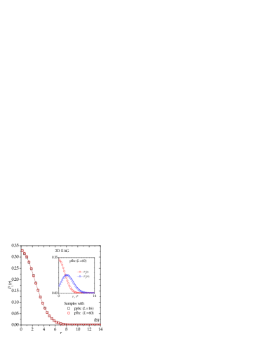
We turn now to the 2D EAG model. Figure 1(b) shows a comparison between the rigidity distributions for systems with ppbc ($L=16$) and with pfbc ($L=60$). Note that finite size effects are not relevant in this case. $P_{L}(r)$ is a continuous function taking appreciable values within a similar range of rigidity as for the 2D EAB model.

Interestingly, the distributions obtained differ substantially from what is obtained by considering locally defined quantities. For each bond $J_{ij}$ of a given sample, we define its local rigidity as $r^{*}_{ij}=U^{*}_{ij}-U$, where $U$ is the GS energy and $U^{*}_{ij}$ is the smallest of the energies of the two configurations obtained by flipping either the spin $\sigma_{i}$ or the spin $\sigma_{j}$. The inset of Fig.1(b) shows, for the 2D EAG model, that the distribution of rigidity $P_{L}(r)$ and the distribution of local rigidity, $P_{L}^{*}(r^{*})$, differ markedly. The local rigidity is closely related to the local fields Marshall1960 ; Klein1963 : The rigidity of a bond is simply the minimum between the absolute local fields, at $T=0$, of spins $i$ and $j$. There is also a factor $2$ that arises from the fact that the rigidity is calculated as an energy difference. The distribution of local fields at $T=0$ has been calculated for the EAG in 2D and 3D, and the curves are very similar to the distribution of local rigidities Boettcher2008 . The rigidity distribution $P_{L}(r)$ [Fig.1(b)] can be well fitted by a Gaussian function,

$$Q(x)=\frac{\sqrt{8/\pi}}{w}\exp\left(-\frac{2x^{2}}{w^{2}}\right),$$ (4)

where $w$ is a constant. For example, for the 2D EAG with ppbc we obtain $w=4.89(1)$.

Figure 2: Map plot of the “average rigidity lattice” for two samples of the 2D (a) EAB and (b) EAG models of $L=60$. In both figures the grayscale is the same and the average rigidity values are 0 (white), 2, 4, 6 and 8 (black).

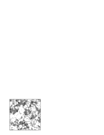
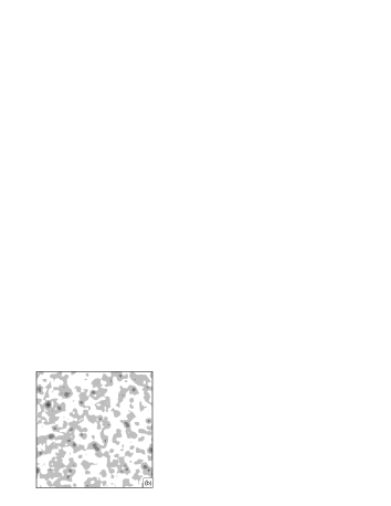
Another important feature of the RS is its spatial distribution. Figure 2 (a) shows a map plot representing the RS of a 2D sample of the EAB model with pfbc and linear size $L=60$. This map plot was generated from an “average rigidity lattice,” where the shade of gray at each site value is given by the average rigidity $\bar{r}$ of the four bonds connecting with this site. It can be observed that bonds with similar rigidity are segregated. Figure 2 (b) shows that this occurs also for a 2D sample of the EAG model and that there are small differences between their spatial rigidity distributions.

Figure 3: (Color online) (a) Rigidity distribution for the 3D EAB model ($L=10$). The inset shows the peaks height of the distribution as function of $1/L$. (b) Rigidity distribution for the 3D EAG model for different lattice sizes as indicated, and for the 2D EAG model (samples of size $L=16$ with ppbc). The inset shows a comparison between $P(r)$ and $P^{*}(r^{*})$ for 3D samples.

Next, we analyze the rigidity distribution $P_{L}(r)$ for the 3D models. Figure 3 (a) shows this distribution for samples of the EAB model of size $L=10$. Now the only possible non-zero rigidity values are $r=4$, $r=8$ and $r=12$, which form the rigid lattice. By extrapolating toward the thermodynamic limit we obtain the following asymptotic distribution: $P(0)=0.45(3)$, $P(4)=0.47(2)$, $P(8)=0.07(1)$ and $P(12)=0.0016(4)$ [see the inset in Fig.3(a)]. Figure 3(b) shows the distribution $P_{L}(r)$ for different lattice sizes of the 3D EAG model. It can again be seen that the shape of $P_{L}(r)$ is unaffected by finite-size effects and that the distribution for $L=8$ can be well fitted by Eq.(4) with $w=5.61(2)$. A comparison with the rigidity distribution of the 2D EAG model shows that the range of nonvanishing values of $r$ in 3D is slightly larger, in agreement with our observations for the 3D EAB model. By comparing $P_{L}(r)$ with the distribution of local rigidity $P_{L}^{*}(r^{*})$ [the inset in Fig.3(b)], it is once again clear that both functions differ substantially. In addition, by means of a qualitative analysis of the rigidity structure, we have observed that a rigidity segregation also emerges in 3D models.

III.2 Percolation of the RS in the EAB model

In this and in the next subsection, we discuss how to use the RS to determine which part of the system has the relevant properties to be called a backbone. But first we need to address the question of which properties are to be considered relevant. We assume that there is a close connection between the topological features of the sets of bonds with a similar rigidity and the equilibrium critical behavior of a given spin-glass model. The main conjecture, proposed in Ref. Roma2010b, , is that, in a system with quenched disorder, it is the rigidity $r_{ij}$, and not the bond strength $J_{ij}$, the quantity that gives the magnitude of the “effective interaction” between spins $i$ and $j$. If this is true, then the backbone of a spin-glass model with a finite (zero) critical temperature should have a percolation cluster with a finite (zero) rigidity value. In addition, within this cluster the correlation length should diverge at the critical point. To address this issue, in the following we analyze the percolation properties of sets with similar rigidities.

It is very difficult to make a direct study of percolation of the different sets in the EA models, because the systems whose RS can be obtained are too small Roma2010b . To overcome this problem, we follow here a more complex, but more conclusive, approach Vogel1998a ; Vogel1998b ; Roma2010b . In a nutshell, what we do, for each structure to be analyzed, is to build a curve of percolation probabilities and to extract a percolation threshold from it. Then we compare this threshold with the estimated size of the corresponding structure in the thermodynamic limit. If this last number is larger than the threshold, we conclude that the structure percolates in the thermodynamic limit. In the following the procedure is explained in more detail for the EAB model, where the rigidity can only take discrete values.

Figure 4: (Color online) Percolation probability $R_{L}^{A}$ for the 2D EAB model (ppbc), for the substructures of the RS with (a) $r=0$ and (b) $r=4$. The insets show $P_{L}(r)$ and the effective thresholds for the percolation criteria $I$ and $A$, as a function of $L^{-1/\nu}$ for (a) $r=0$ and (b) $r=4$.

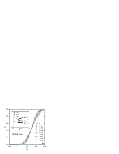
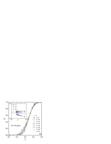
For the set of bonds having the same rigidity $r$, we define $R^{U}_{L}(h_{r})$ and $R^{I}_{L}(h_{r})$ Yonezawa1989 as the probabilities that this set percolates along at least one lattice direction, and simultaneously along all independent lattice directions, respectively, if the size of the set is between $h_{r}$ and $h_{r}+\Delta h$ (sizes are given as fractions over the total number of bonds). We also define the arithmetic mean of these quantities as $R^{A}_{L}(h_{r})\equiv[R^{U}_{L}(h_{r})+R^{I}_{L}(h_{r})]/2$.

Figures 4(a) and 4(b) show, for the 2D EAB model with ppbc, the percolation probability function $R^{A}_{L}$ of the substructures with $r=0$ and $r=4$, respectively, for different lattice sizes (we show only the percolation criterion $A$ because for this model it is the quantity less sensitive to finite size effects). Calculations were performed using the algorithm of Hoshen-Kopelman Hoshen1976 . As for small lattice sizes the fractions of rigid bonds such as $h_{0}$ and $h_{4}$ have a very wide distribution Roma2010b , the curves in these figures extend over almost the entire range of this variable, from 0 to 1. In all cases, we have used a bin width of $\Delta h=0.05$. Error bars were calculated using a bootstrap method numerical but they are omitted when they are smaller than the symbol size.

Although the crossing points that define the percolation thresholds are easy to establish, we perform for each set a standard analysis of the data, in order to improve the accuracy of the values obtained Yonezawa1989 ; Roma2010b . First, each curve is fitted with an error function using a least-mean-squares method. Then the concentration at which the slope of the fitting curve is largest is taken as an effective threshold $h^{\mathcal{X}}_{rc}(L)$, where $\mathcal{X}$ denotes the percolation criterion used: $U$, $I$ or $A$. $h^{\mathcal{X}}_{rc}(L)$ is expected to follow the law Stauffer1985

$$h^{\mathcal{X}}_{rc}(L)=h_{rc}+C^{\mathcal{X}}L^{-1/\nu},$$ (5)

where $C^{\mathcal{X}}$ is a non-universal constant and $\nu$ is the critical exponent associated to the correlation length. As in a previous work Roma2010b , for the 2D EAB model we have used $\nu=4/3$, corresponding to 2D random percolation Stauffer1985 .

The inset in Fig. 4(a) shows the mean fraction of bonds with $r=0$, $P_{L}(0)$, and the effective thresholds for the three percolation criteria. To calculate an estimate of the percolation thresholds at the thermodynamic limit, we have extrapolated the data by means of a linear fit. We obtain the following limits: $P(0)=0.49(1)$, $h_{0c}^{I}=0.506(6)$, $h_{0c}^{U}=0.48(1)$ and $h_{0c}^{A}=0.484(8)$ [we determine a somewhat different limit of $P(0)$ from the one calculated above, because here the fit is carried out using $L^{-1/\nu}$]. These values are too close to be useful to decide whether the substructure with $r=0$ percolates. Unfortunately, even though larger sizes are available, the situation is very similar in the case of the 2D EAB model with pfbc. On the other hand, for the substructure with $r=4$, we obtain the following: $P(4)=0.483(6)$, $h_{4c}^{I}=0.53(1)$, $h_{4c}^{U}=0.51(2)$ and $h_{4c}^{A}=0.52(1)$ [see the inset in Fig. 4 (b)]. If the percolation threshold $h_{4c}^{U}$ is discarded, because of large finite-size effects, the conclusion is that this substructure has not percolated. The structure with $r=8$ has not been analyzed because its size is too small.

For 3D lattices we have used $\nu=0.9$, and only the percolation criterion I because the others are affected by large finite size effects. In the thermodynamic limit we obtain the following: $P(0)=0.45(1)>h_{0c}^{I}=0.24(1)$ and $P(4)=0.48(2)>h_{4c}^{I}=0.30(1)$. Thus, unlike what happens in 2D, in 3D both sets with $r=0$ and $r=4$ percolate. The simultaneous percolation of two different structures in 3D systems has also been found in other contexts Isichenko1992 .

It is interesting to note that the percolation properties of the set of bonds with $r=4$ is very similar to what has been found for the whole rigid lattice Roma2010b , which comprises all bonds with $r\geq 4$. This is because bonds with $r=8$ in 2D, and with $r=8$ and $r=12$ in 3D, can only form small and compact clusters that fill the interstices of the larger substructure with $r=4$.

The idea that the structure with $r=4$ dominates the physical behavior of the backbone is supported by the analysis of the function $F_{J}(r,T)$, defined as the mean value of the fraction of bonds with rigidity $r$ which, at temperature $T$, have the same condition (satisfied or frustrated) as in the GS. It is easy to see that, when $T\to 0$, those bonds with non zero rigidity frozen and then $F_{J}(r,T)\to 1$, while for $T\to\infty$ the mean fraction $F_{J}(r,T)\to 1/2$. Figure 5(a) shows the sample average of this fraction, $F(r,T)$, for the 2D ($L=16$ with ppbc) and the 3D ($L=8$) EAB models [as bonds with $r=0$ do not have a defined condition on the GS, we have set $F(0,T)=1/2$ for any $T$] Note2 . With decreasing temperature, Fig. 5(a) shows that bonds with large rigidity freeze faster than those with small rigidity. This gives support to our conjecture that it is the rigidity $r_{ij}$, and not the bond strength $J_{ij}$, that gives the magnitude of the effective interaction between spins $i$ and $j$ (recall that in the EAB we have $|J_{ij}|=1$). In particular for the 3D EAB model and close to the critical temperature $T_{c}\approx 1.12$ Katzgraber2006 , we see that bonds with $r=12$ and $8$ are almost completely frozen, while only the bonds with $r=4$ are affected by thermal fluctuations. But it is precisely this substructure that percolates in the thermodynamic limit. Thus, it is reasonable to assume that, at the critical point, it is in this region that there is a divergence of the correlation length.

Figure 5: (Color online) $F(r,T)$ as function of $r$ for (a) the 2D and the 3D EAB models and for (b) the 2D and the 3D EAG models. Curves are given for different temperatures as indicated.

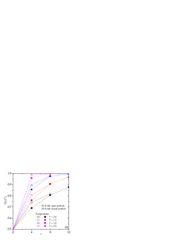
Figure 5(b) shows the same function $F(r,T)$ for the 2D and the 3D EAG models, for lattice sizes of $L=16$ and $L=8$, respectively. We observe a similar behavior to that of the EAB, but now for models with continuous bond and rigidity distributions. Notice that close to $T_{c}\approx 0.95$ Katzgraber2006 , bonds with a rigidity between $r\approx 2$ and $r\approx 4$ are affected by thermal fluctuations.

Remarkably, $F(r,T)$ is very well fitted by the functional form $1/(1+\exp(-ar/T))$, where the parameter $a$ is close to $2$ for all models. This represents the probability that a system with only two levels, with an energy difference of $a\,r$, is in the GS. We emphasize that this result is not a trivial consequence of the definition of bond rigidity, because the $r$ values are a measure of the energy difference between the GS and the low-excitation levels (where entropic effects are not taken into account), whereas the function $F(r,T)$ is calculated in equilibrium, where the dynamics takes place at finite temperature and the system explores configurations corresponding to highly excited levels.

III.3 Percolation of the RS in the EAG model

To study percolation in the EAG model, we choose to break the RS into two sets, one formed by the bonds with rigidity $r\geq r_{\textrm{min}}$, $\Omega(r_{\textrm{min}})$, and another set $\Omega^{*}(r_{\textrm{min}})$ comprising the remaining bonds, where $r_{\textrm{min}}$ is a given rigidity value. This choice is motivated by the existence of the rigid and the flexible lattices in EAB systems. Besides, the study of the percolation of smaller structures (centered around given values of $r$) is not possible in our case because the size of the systems used is too small.The sizes of the sets $\Omega(r_{\textrm{min}})$ and $\Omega^{*}(r_{\textrm{min}})$, denoted as $h_{x}$ and $h_{x}^{*}=1-h_{x}$, respectively, have large variations for different samples. However, in the previous section we have shown that the rigidity distribution $P_{L}(r)$ shows almost no dependence on sample size for the EAG, and thus the same happens for the sample averages of $h_{x}$, denoted as $X(r_{\textrm{min}})$.

Figure 6: (Color online) Percolation probability $R_{L}^{A}$ curves for (a) the 2D (ppbc) and (b) the 3D EAG models for $r_{\textrm{min}}=2.5$ and $r_{\textrm{min}}=4$, respectively. The insets show for each model, the comparison between $h_{xc}$ and $X$, and between $h^{*}_{xc}$ and $1-X$, as functions of $r_{\textrm{min}}$.

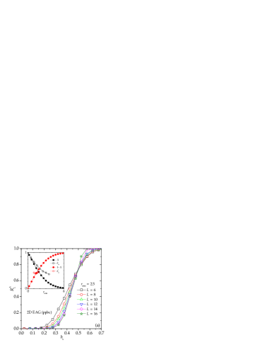
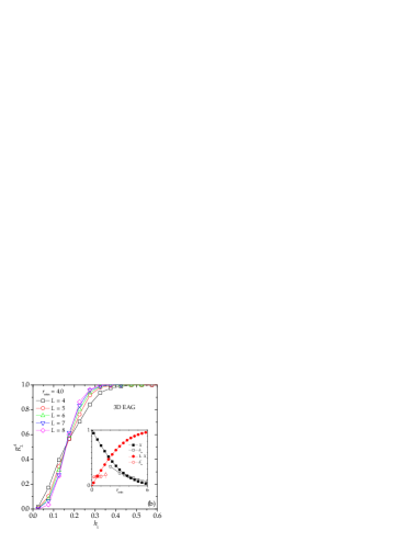
Similarly to what we have done for the EAB models, for each value ​​of $r_{\textrm{min}}$ we calculate a percolation threshold $h_{xc}(r_{\textrm{min}})$ and then we compare this number to the corresponding $X(r_{\textrm{min}})$: If $h_{xc}<X$ the set $\Omega$ percolates. Figure 6(a) shows the curves of the percolation probability $R_{L}^{A}$ for the 2D EAG model with ppbc for $r_{\textrm{min}}=2.5$. In this case the percolation threshold is (calculated as in the previous section) $h_{xc}(2.5)=0.48(2)$, and $X(2.5)=0.31(1)$; therefore ,the set $\Omega(2.5)$ does not percolate. For too-small or too-large values of $r_{\textrm{min}}$ the calculation of the threshold becomes impossible because of the small size of the corresponding sets in the samples available to us.

The inset in Fig. 6(a) shows the comparison between $h_{xc}$ and $X$ as function of $r_{\textrm{min}}$. Extrapolating we can deduce that, for the 2D EAG model with ppbc, the set $\Omega(r_{\textrm{min}})$ percolates when $r_{\textrm{min}}\to 0$, which is consistent with a vanishing $T_{c}$ for this model (this is similar to what happens for the 2D EAB model).

Now we consider the complementary set $\Omega^{*}(r_{\textrm{min}})$ composed by the bonds with $r<r_{\textrm{min}}$. For this set the percolation threshold is denoted as $h^{*}_{xc}(r_{\textrm{min}})$. Comparing this quantity with the fraction $1-X(r_{\textrm{min}})$, we can find whether the bonds with the lowest rigidity percolate in the thermodynamic limit. The inset in Fig. 6 (a) shows this comparison. As we can see for the 2D EAG model, when $r_{\textrm{min}}\gtrsim 1.3$ the set $\Omega^{*}(r_{\textrm{min}})$ percolates.

For the 3D EAG model the situation differs. Figure 6(b) shows that, for the set $\Omega(r_{\textrm{min}})$, the percolation probability $R_{L}^{A}$ curves for $r_{\textrm{min}}=4$ intersect at $h_{xc}(4)=0.16(1)$, a value very close to $X(4)=0.163(1)$. In turn, the inset shows that $h_{xc}$ and $X$ cross at a value of $r_{\textrm{min}}$ close to 4. On the other hand, for the complementary set $\Omega^{*}(r_{\textrm{min}})$, the inset in Fig. 6(b) also shows that the curves of $h^{*}_{xc}$ and $1-X$ cross at $r_{\textrm{min}}\approx 0.6$. Thus, for $0.16<r_{min}<4$ both sets, $\Omega(r_{\textrm{min}})$ and $\Omega^{*}(r_{\textrm{min}})$, percolate.

III.4 The backbone of the EAG models

Figure 7: (Color online) Rigidity distributions $P_{L}(r)$, $P_{L}^{S}(r)$, and $P_{L}^{F}(r)$ (see text) for (a) the 2D ($L=16$ with ppbc) and (b) the 3D ($L=8$) EAG models. The vertical dotted lines marks the value of $r_{\textrm{min}}=1.3$.

In the previous sections we have shown that the percolation properties of the RS for the EAG and the EAB models are very similar. In the following we show that there are values of $r_{\textrm{min}}$ for which the physical properties of the sets $\Omega(r_{\textrm{min}})$ and $\Omega^{*}(r_{\textrm{min}})$ are equivalent, respectively, to those of the backbone and its complement in EAB models.

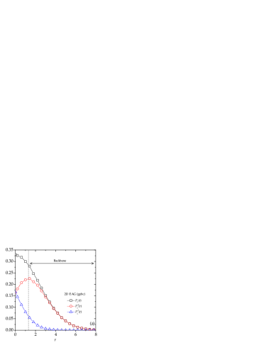
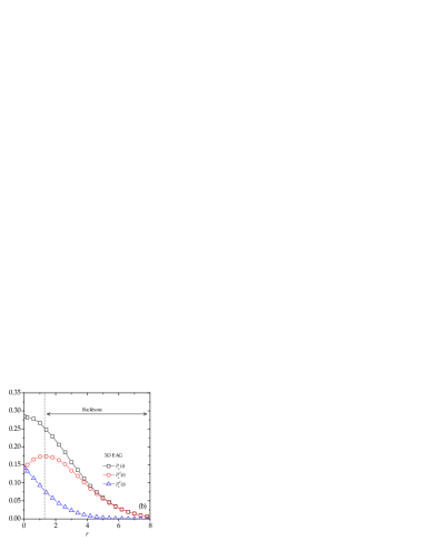
Figures 7(a) and 7(b) show, for the 2D and the 3D EAG models, a comparison between the rigidity distributions for all bonds, $P_{L}(r)$, for the bonds that are satisfied in the GS, $P_{L}^{S}(r)$, and for the bonds that are frustrated in the GS, $P_{L}^{F}(r)$. Obviously the distributions must satisfy $P_{L}(r)=P_{L}^{S}(r)+P_{L}^{F}(r)$. Note that the distributions $P_{L}^{S}(r)$ and $P_{L}^{F}(r)$ are not normalized to unity because their integrals are equal to, respectively, the fractions of satisfied and frustrated bonds of the GS. In both cases, for large values of $r_{\textrm{min}}$, almost all the bonds in the set $\Omega(r_{\textrm{min}})$ are satisfied in the GS. However, even though with decreasing $r_{\textrm{min}}$ the size of the set $\Omega(r_{\textrm{min}})$ increases, the fraction of frustrated bonds is rather small. A change of trend occurs when the $P_{L}^{S}(r)$ distribution reaches its maximum: For smaller values of $r_{\textrm{min}}$ the set $\Omega(r_{\textrm{min}})$ begins to incorporate highly frustrated regions. Remarkably, this maximum happens approximately at $r_{\textrm{min}}\approx 1.3$ for both, the 2D and the 3D EAG models.

Interestingly, for the 2D EAG model we have shown in the previous subsection that at $r_{\textrm{min}}=1.3$ the complementary set $\Omega^{*}(1.3)$ is very close to the percolation thresholds, whereas the set $\Omega(1.3)$ does not percolate. Therefore, it seems reasonable to define the backbone of this system as the set $\Omega(1.3)$. This choice gives a backbone having the $60\%$ of the bonds of the system and a fraction of frustrated bonds in the GS of only $0.085$.

Figure 8: (Color online) Average energies per bond $u(T)$, $u_{\Omega}(T)$ and $u_{\Omega^{*}}(T)$ (see text) for (a) the 2D ($L=16$ with ppbc) and (b) the 3D ($L=8$) EAG models. In both cases $r_{\textrm{min}}=1.3$ was chosen. Insets show the curve of $u_{\Omega^{*}}(T)$ for different values of $r_{\textrm{min}}$.

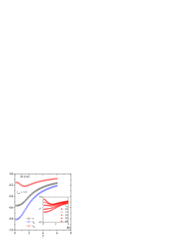
In the EAB model, several observables behave differently when they are calculated within or outside of the backbone, such as the average energy per bond Roma2010b . For example, when this quantity is evaluated outside the backbone, it has a minimum at low temperature. To perform a similar analysis for the EAG models, we define $u(T)$, $u_{\Omega}(T)$, and $u_{\Omega^{*}}(T)$ as the average energies per bond at temperature $T$ of, respectively, the whole system and the sets $\Omega$ and $\Omega^{*}$ for a given $r_{\textrm{min}}$.

Figure 8(a) shows, for the 2D EAG model, these energies as functions of $T$ for $r_{\textrm{min}}=1.3$. Just as in the 2D EAB model Roma2010b , there is a very broad minimum in the curve of $u_{\Omega^{*}}(T)$. For higher (lower) values of $r_{\textrm{min}}$, the inset in that figure shows that the minimum disappears (becomes narrower).

For the 3D EAG model, Fig. 8(b) and its inset show that for some values of $r_{\textrm{min}}$ around $1.3$, the curves of $u_{\Omega^{*}}(T)$ display a minimum. Our calculations suggest that a suitable backbone could be defined in the range $[0.6-2.0]$, since all these structures have similar topological characteristics. However, in the following we use $r_{\textrm{min}}=1.3$ to define the backbone of the 3D EAG model. This set has $64\%$ of the bonds of the system and a fraction of frustrated bonds in the GS of $0.163$.

Note that, whereas the percentage of bonds comprising the backbone is only slightly larger in 3D than in 2D, in 3D the fraction of those bonds that are frustrated is twice that in 2D. The same is obtained for the EAB models: The backbone (defined as the set of bonds with rigidity $r\geq 4$) comprises approximately $52\%$ of the system in 2D and $54\%$ in 3D, and the fraction of frustrated bonds is $0.05$ in 2D and $0.1$ in 3D Roma2010b .

Finally, we analyze the internal structure of the backbone by studying the cluster number distribution, $n_{s}$, i.e., the number of clusters of size $s$. For the random bond percolation at the critical concentration, it is expected that this distribution follows a power law

$$n_{s}\propto s^{-\tau},$$ (6)

where $\tau$ is a critical exponent Stauffer1985 . Because large samples are needed, in 2D we have restricted our analysis to lattices with pfbc of size $L=60$. Figure 9(a) shows, for the 2D EAB model, the cluster number distribution calculated for a range of $h_{x}$ centered at $0.55$, the mean fraction of bonds with rigidity $r\geq 4$. Fitting the curve we obtain $\tau=1.95(5)$. On the other hand, we have also calculated this distribution for the backbone of the 2D EAG model ($r_{\textrm{min}}=1.3$), for two different ranges of $h_{x}$: one centered at $h^{*}_{xc}(1.3)=0.68$ and another at $X(1.3)=0.6$ [see the inset in Fig. 6 (a)]. For these ranges we obtain, respectively, $\tau=2.03(8)$ and $\tau=1.98(4)$. Whatever the model or the range, the exponent values are very close to $\tau=187/91\approx 2.05$, the corresponding exponent for the 2D random percolation universality class Stauffer1985 .

Figure 9: (Color online) Cluster number distributions for the EAB and EAG models for (a) 2D ($L=60$ with pfbc) and (b) 3D ($L=8$) lattices. The distributions are calculated for different ranges.

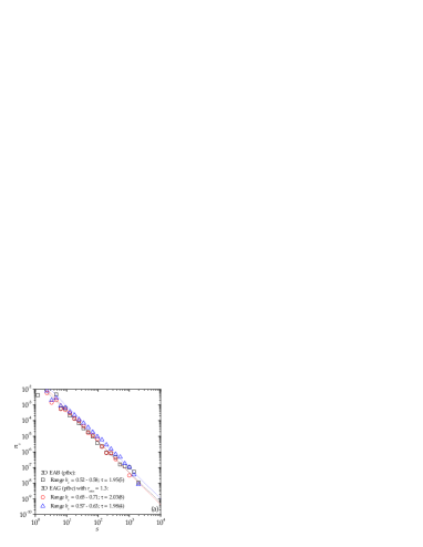
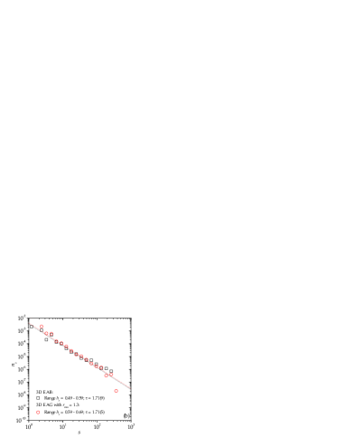
For 3D systems Fig. 9(b) shows the cluster number distributions for both the 3D EAB model for a range centered at $0.54$ (the mean fraction of bonds with rigidity $r\geq 4$), and the 3D EAG model for a range centered at $X(1.3)=0.64$ [see the inset in Fig. 6 (b)]. We obtain, respectively, $\tau=1.71(9)$ and $\tau=1.71(5)$, values that clearly differ from the accepted exponent $\tau=2.2$ of random percolation in 3D Stauffer1985 . This difference is presumably due to the fact that, unlike the 2D case, here the mean size of the backbone tends to a value far from the percolation threshold. Nevertheless, for the small sizes considered, we see that the cluster number distributions for both 3D models follows a power law with the same exponent. These results show that the internal structures of the backbones of systems with bimodal and Gaussian bond distributions are similar.

IV Discussion and conclusions

It has recently been shown that in EA models with a discrete distribution of bonds, and therefore with a degenerate ground state, it is possible to find a set of bonds, called backbone, which is closely related to the heterogeneities of the GS structure, and that may be used to have a better understanding of the physical properties of such systems. More specifically, the backbone and its complement seem to influence both the equilibrium and the out-of-equilibrium dynamics of the EAB models Roma2006 ; Roma2007b ; Roma2010a ; Roma2010b ; Rubio2010a ; Rubio2010b . Here we have shown that in systems with continuous distributions of bonds it is possible to define a continuous version of bond rigidity, which in turn leads to the definition of a backbone. Even though there is a certain degree of arbitrariness in the choice of the threshold rigidity value that defines the backbone, we have shown here that the resulting structure shares most of the topological characteristics and physical properties of the backbone of EAB systems.

We have also argued that the reason why sets of bonds with different rigidities (as the backbone and its complement) have different physical properties, is that the rigidity provides more physical information than the bond strength. It could even be thought that the rigidity $r_{ij}$ in some way encodes the magnitude of the effective interaction between spins $\sigma_{i}$ and $\sigma_{j}$. To provide additional evidence that the backbone is not directly related to bond strengths, we calculate for the 2D and the 3D EAG models the probability distribution that a bond has strength $J$ and rigidity $r$. Dividing this function by $D_{\mathrm{G}}(J)$, the Gaussian bond distribution, we obtain the conditional probability density $W(J,r)$ which, for fixed value of $r$, is normalized to unity.

Figures 10(a) and 10(b) show the map plots of $W(J,r)$ for, respectively, the 2D and the 3D EAG models. For relatively large values of $|J|$ and $r$ both distributions develop two arms. Thus, for most of the bonds in this range their strength is proportional to their rigidity. This is to be expected, since these bonds must be surrounded by many others of lower strength, and then the changes in the GS energy (and therefore in the rigidity), produced by changing the condition of a bond of great magnitude, should depend primarily on the value of $|J|$. In other words, the rigidity of a high-strength bond seems to be, on average, a trivial quantity Note1 .

Figure 10: Map plot of the conditional probability density $W(J,r)$ for (a) the 2D ($L=60$ with pfbc) and (b) the 3D ($L=8$) EAG models. The horizontal dotted lines marks the value of $r_{\textrm{min}}=1.3$.

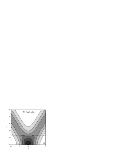
On the other hand, for intermediate and low values of $|J|$ and $r$, the function $W(J,r)$ for both the 2D EAG and the 3D EAG models has a square shape in which the approximate proportionality between the strength of a given bond and its rigidity is lost. For example in the 3D case, Fig. 10(b) shows that $W(J,r)$ is almost constant on the region given by $-1\lesssim J\lesssim 1$ and $1\lesssim r\lesssim 2$. The same applies to bonds with $|J|\approx 1$ which have, with equal probability, a rigidity between $0\leq r\lesssim 2$. These examples show that the intermediate region of parameters, where many of the bonds that make up the backbone are located, and where the thermal critical (in 3D) fluctuations are important, is nontrivial.

As mentioned in Sec. I, temperature chaos McKay1982 ; Bray1987 ; Rizzo2003 ; Parisi2010 is an important issue which must be reconciled with this phenomenological backbone picture. If our results were interpreted as a suggestion that ground state excitations can have an influence on finite temperature dynamics, the phenomenon of temperature chaos would imply that the backbone can only be relevant for the physics of small systems. However, what we argue here is that the system can be divided into two macroscopic sectors where the effective interactions between spins, which we assume are temperature-independent quantities, seem to differ markedly. The GS and its excitations are only used as tools to find which spins and bonds comprise those sectors. Once the sample has been so divided, the information about the states is no longer necessary. In other words, we do not make any assumptions about the magnitude of the overlap between states at finite temperature and the GS and its excitations. Therefore, in principle, we would expect that this physical separation of the system is also valid for macroscopic samples. However, this conjecture can only be confirmed by performing simulations in those rare small samples where temperature chaos has been shown to be present Katzgraber2007 ; Fernandez2013 .

The topological characteristics of the backbone may also be relevant for a better understanding of the physical behavior of other random systems. For example, Tsomokos et al. Tsomokos2011 predict that if the backbone of the 2D EAB model does not percolate, in the random-field toric code model there may exist a new intermediate quantum phase where topological and spin-glass order coexist. Our calculations suggest that this could also be the case for both 2D models. In addition, in a recent study of the out-of-equilibrium dynamics of the 2D $\pm J$ Potts model at low-temperature, numerical evidence has been found that hints at the existence of an underlying backbone structure for this system Ferrero2012 . Unfortunately, the RS studied there is defined only for models with Ising spins (the $q=2$ case in the $\pm J$ Potts model correspond to the EAB model). Although a general procedure to obtain the backbone of an arbitrary system has not yet been found, we believe that the progress made here represents a significant step in this direction. We hope that a further generalization of the rigid structure analyzed here will make it possible to identify the backbone of more complex disordered models.