MCMC Bayesian Estimation in FIEGARCH Models

Abstract

Bayesian inference for fractionally integrated exponential generalized autoregressive conditional heteroskedastic (FIEGARCH) models using Markov Chain Monte Carlo (MCMC) methods is described. A simulation study is presented to access the performance of the procedure, under the presence of long-memory in the volatility. Samples from FIEGARCH processes are obtained upon considering the generalized error distribution (GED) for the innovation process. Different values for the tail-thickness parameter $\nu$ are considered covering both scenarios, innovation processes with lighter ($\nu<2$) and heavier ($\nu>2$) tails than the Gaussian distribution ($\nu=2$). A sensitivity analysis is performed by considering different prior density functions and by integrating (or not) the knowledge on the true parameter values to select the hyperparameter values.

Key words: Bayesian inference, MCMC, FIEGARCH processes, Long-range dependence.

1 Introduction

ARCH-type (Autoregressive Conditional Heteroskedasticity) and stochastic volatility (Breidt et al., 1998) models are commonly used in financial time series modeling to represent the dynamic evolution of volatilities. By ARCH-type models we mean not only the ARCH model proposed by Engle (1982) but also several generalizations that were lately proposed.

Among the most popular generalizations of the ARCH model is the generalized ARCH (GARCH) model, introduced by Bollerslev (1986), for which the conditional variance depends not only on the $p$ past values of the process (as in the ARCH model), but also on the $q$ past values of the conditional variance. Although the ARCH and GARCH models are widely used in practice, they do not take into account the asymmetry in the volatility, that is, the fact that volatility tends to rise in response to “bad” news and to fall in response to “good” news. As an alternative, Nelson (1991) introduces the exponential GARCH (EGARCH) model. This model not only describes the asymmetry on the volatility, but also have the advantage that the positivity of the conditional variance is always attained since it is defined in terms of the logarithm function.

The fractionally integrated EGARCH (FIEGARCH) and fractionally integrated GARCH (FIGARCH) models proposed, respectively, by Bollerslev and Mikkelsen (1996) and Baillie et al. (1996), generalize the EGARCH (Nelson, 1991) and the GARCH (Bollerslev, 1986) models, respectively. FIEGARCH models have not only the capability of modeling clusters of volatility (as ARCH and GARCH models do) and capturing its asymmetry (as the EGARCH model does) but they also take into account the characteristic of long memory in the volatility (as the FIGARCH model does). The non-stationarity of FIGARCH models (in the weak sense) makes this class of models less attractive for practical applications. Another drawback of the FIGARCH models is that we must have $d\geq 0$ and the polynomial coefficients in its definition must satisfy some restrictions so the conditional variance will be positive. FIEGARCH models do not have this problem since the variance is defined in terms of the logarithm function, moreover, they are weak stationary whenever the long memory parameter $d$ is smaller than 0.5 (Lopes and Prass, 2013).

A complete study on the theoretical properties of FIEGARCH processes is presented in Lopes and Prass (2013). The authors also conduct a simulation study to analyze the finite sample performance of the quasi-maximum likelihood (QML) procedure on parameter estimation. The QML procedure became popular for two main reasons. First, the expression for the quasi-likelihood function is simpler for the Gaussian case than when considering, for example, the Student’s $t$ or the generalized error distribution (GED). Second, since the parameters of the distribution function are not estimated, the dimension of the optimization problem is reduced. On the other hand, the results in Lopes and Prass (2013) indicate that, although the QML presents a relatively good performance when the sample size is 2000 and the estimation improves as the sample size increases, it does so very slowly.

In this work we propose the use of Bayesian methods using Monte Carlo simulation techniques on the estimation of the FIEGARCH model parameters. This procedure is usually considered to analyze financial time series assuming stochastic volatility models (see, for example, Meyer and Yu, 2000), mostly because of the difficulty on applying traditional statistical techniques due to the complexity of the likelihood function. To generate samples from the joint posterior distribution for the parameters of interest we use MCMC (Markov Chain Monte Carlo) methods as the Gibbs Sampling algorithm (see, for example, Gelfand and Smith, 1990; Casela and George, 1992) or the Metropolis-Hastings algorithm (see, for example, Smith and Roberts, 1993; Chib and Greenberg, 1995). These samples are generated from all conditional posterior distributions for each parameter given all the other parameters and the data.

A simulation study is conducted to access the finite sample performance of the procedure proposed here, under the presence of long-memory in the volatility. The samples from FIEGARCH processes are obtained upon considering the GED for the innovation process. Taking into account that financial time series are usually characterized by heavy tailed distributions, different values for the tail-thickness parameter $\nu$ are considered covering both scenarios: innovation processes with lighter and heavier tails than the Gaussian distribution. A sensitivity analysis is performed by considering different prior density functions and by integrating (or not) the knowledge on the true parameter values to select the hyperparameter values.

The paper is organized as follows. In Section 2 a review on the definition and main properties of FIEGARCH processes is presented. Section 3 describes the parameter estimation procedure when Bayesian inference using MCMC is considered. Section 4 describes the steps used in the simulation study, such as the data generating process, the prior selection procedure and the performance measures considered. This section also reports the simulation results. Section 5 concludes the paper.

2 FIEGARCH Processes

Let $(1-\mathcal{B})^{-d}$ be the operator defined by its Maclaurin series expansion, namely,

$$(1-\mathcal{B})^{-d}=\sum_{k=0}^{\infty}\frac{\Gamma(k+d)}{\Gamma(k+1)\Gamma(d)}:=\sum_{k=0}^{\infty}\tau_{d,k}\,\mathcal{B}^{k},$$ (1)

where $\tau_{d,k}:=\frac{\Gamma(k+d)}{\Gamma(k+1)\Gamma(d)}$, for all $k\geq 1$, $\Gamma(\cdot)$ is the gamma function and $\mathcal{B}$ is the backward shift operator defined by $\mathcal{B}^{k}(X_{t})=X_{t-k}$, for all $k\in\mathds{N}$.

Assume that $\alpha(\cdot)$ and $\beta(\cdot)$ are polynomials of order $p$ and $q$, respectively, defined by

$$\alpha(z)=\sum_{i=0}^{p}(-\alpha_{i})z^{i}\quad\mbox{ and}\quad\beta(z)=\sum_{j=0}^{q}(-\beta_{j})z^{j},$$ (2)

with $\alpha_{0}=\beta_{0}=-1$. If $\alpha(\cdot)$ and $\beta(\cdot)$ have no common roots and $\beta(z)\neq 0$ in the closed disk $\{z:|z|\leq 1\}$, then the function $\lambda(\cdot)$, defined by

$$\lambda(z)=\frac{\alpha(z)}{\beta(z)}(1-z)^{-d}:=\sum_{k=0}^{\infty}\lambda_{d,k}z^{k},\quad\mbox{ for all }|z|<1,$$ (3)

is analytic in the open disc $\{z:|z|<1\}$, for any $d>0$, and in the closed disk $\{z:|z|\leq 1\}$, whenever $d\leq 0$. Therefore, $\lambda(\cdot)$ is well defined and the power series representation in (3) is unique. More specifically, the coefficients $\lambda_{d,k}$, for all $k\in\mathds{N}$, are given by (see Lopes and Prass, 2013)

$$\lambda_{d,0}=1\quad\mbox{ and}\quad\lambda_{d,k}=-\alpha_{k}^{*}+\sum_{i=0}^{k-1}\lambda_{i}\sum_{j=0}^{k-i}\beta_{j}^{*}\delta_{d,k-i-j},\ \mbox{ for all }\ k\geq 1,$$ (4)

where

$$\alpha_{m}^{*}:=\left\{\begin{array}[]{ccc}\alpha_{m},&\mbox{ if}&0\leq m\leq p;\vspace{.3cm}\\ 0,&\mbox{ if}&m>p;\end{array}\right.\quad\beta_{m}^{*}:=\left\{\begin{array}[]{ccc}\beta_{m},&\mbox{ if}&0\leq m\leq q;\vspace{.3cm}\\ 0,&\mbox{ if}&m>q;\end{array}\right.$$ (5)

and $\delta_{d,j}:=\tau_{-d,j}$, for all $j\in\mathds{N}$, are the coefficients obtained upon replacing $-d$ by $d$ in (1), that is

$$\sum_{k=0}^{\infty}\delta_{d,k}\mathcal{B}^{k}:=\sum_{j=0}^{\infty}\tau_{-d,j}\mathcal{B}^{j}=(1-\mathcal{B})^{d}.$$

Let $\theta,\gamma\in\mathds{R}$ and $\{Z_{t}\}_{t\in\mathds{Z}}$ be a sequence of independent and identically distributed (i.i.d.) random variables, with zero mean and variance equal to one. Assume that $\theta$ and $\gamma$ are not both equal to zero and define $\{g(Z_{t})\}_{t\in\mathds{Z}}$ by

$$g(Z_{t})=\theta Z_{t}+\gamma[|Z_{t}|-\mathds{E}(|Z_{t}|)],\quad\mbox{ for all }t\in\mathds{Z}.$$ (6)

It follows that (see Lopes and Prass, 2013) $\{g(Z_{t})\}_{t\in\mathds{Z}}$ is a strictly stationary and ergodic process. Moreover, since $\mathds{E}(Z_{0}^{2})<\infty$, then $\{g(Z_{t})\}_{t\in\mathds{Z}}$ is also weakly stationary with mean zero (therefore a white noise process) and variance $\sigma^{2}_{g}$ given by

$$\sigma^{2}_{g}=\theta^{2}+\gamma^{2}-[\gamma\mathds{E}(|Z_{0}|)]^{2}+2\,\theta\,\gamma\,\mathds{E}(Z_{0}|Z_{0}|).$$ (7)

Now, for any $d<0.5$ and $\omega\in\mathds{R}$, let $\{X_{t}\}_{t\in\mathds{Z}}$ be the stochastic process defined by

$$X_{t}\, =\,\sigma_{t}Z_{t},$$ (8)

$$\ln(\sigma_{t}^{2}) \,=\,\omega+\frac{\alpha(\mathcal{B})}{\beta(\mathcal{B})}(1-\mathcal{B})^{-d}g(Z_{t-1})$$

$$=\omega+\sum_{k=0}^{\infty}\lambda_{d,k}g(Z_{t-1-k}),\quad\mbox{ for all }t\in\mathds{Z}.$$ (9)

Then $\{X_{t}\}_{t\in\mathds{Z}}$ is a Fractionally Integrated EGARCH process, denoted by FIEGARCH$(p,d,q)$ (Bollerslev and Mikkelsen, 1996).

The properties of FIEGARCH$(p,d,q)$ processes, with $d<0.5$, are given below (the proofs of these properties can be found in Lopes and Prass, 2013). Henceforth GED$(\nu)$ denotes the generalized error distribution with tail thickness parameter $\nu$.

Proposition 1.

Let $\{X_{t}\}_{t\in\mathds{Z}}$ FIEGARCH$(p,d,a)$ process. Then the following properties hold:

1. $\{\ln(\sigma_{t}^{2})\}_{t\in\mathds{Z}}$ is a stationary (weakly and strictly) and an ergodic process and the random variable $\ln(\sigma_{t}^{2})$ is almost surely finite, for all $t\in\mathds{Z}$;

2. if $d\in(-1,0.5)$ and $\alpha(z)\neq 0$, for $|z|\leq 1$, the process $\{\ln(\sigma_{t}^{2})\}_{t\in\mathds{Z}}$ is invertible;

3. $\{X_{t}\}_{t\in\mathds{Z}}$ and $\{\sigma_{t}^{2}\}_{t\in\mathds{Z}}$ are strictly stationary and ergodic processes;

4. if $\{Z_{t}\}_{t\in\mathds{Z}}$ is a sequence of i.i.d. GED$(\nu)$ random variables, with $v>1$, zero mean and variance equal to one, then $\mathds{E}(X_{t}^{r})<\infty$ and $\mathds{E}(\sigma_{t}^{2r})<\infty$, for all $t\in\mathds{Z}$ and $r>0$.

3 Parameter Estimation: Bayesian Inference using MCMC

Let $\nu$ be the parameter (or vector of parameters) associated to the probability density function of $Z_{0}$ and denote by

• $\boldsymbol{\eta}=(\nu,d,\theta,\gamma,\omega,\alpha_{1},\cdots,\alpha_{p},\beta_{1},\cdots,\beta_{q})^{\prime}:=(\eta_{1},\eta_{2},\cdots,\eta_{5+p+q})^{\prime}$ the vector of unknown parameters in (9);

• $\boldsymbol{\eta}_{(-i)}$ the vector containing all parameters in $\boldsymbol{\eta}$ except $\eta_{i}$, for each $i\in\{1,\cdots,5+p+q\}$;

• $p_{\mbox{\tiny$Z$}}(\cdot|\nu)$ the probability density function of $Z_{0}$ given $\nu$;

• $\mathcal{F}_{t}$ the $\sigma$-algebra generated by $\{Z_{s}\}_{s\leq t}$;

• $p_{\mbox{\tiny$X_{t}$}}(\cdot|\boldsymbol{\eta},\mathcal{F}_{t-1})$ the probability density function of $X_{t}$ given $\boldsymbol{\eta}$ and $\mathcal{F}_{t-1}$, for all $t\in\mathds{Z}$.

From (9) it is evident that, given $\boldsymbol{\eta}$, $\sigma_{t}$ is a $\mathcal{F}_{t-1}$-measurable random variable. Moreover, since $X_{t}=\sigma_{t}Z_{t}$ and $p_{\mbox{\tiny$Z$}}(\cdot|\nu,\mathcal{F}_{t-1})=p_{\mbox{\tiny$Z$}}(\cdot|\nu)$, the following equality holds

$$p_{\mbox{\tiny$X_{t}$}}(x_{t}|\boldsymbol{\eta},\mathcal{F}_{t-1})=\frac{1}{\sigma_{t}}p_{\mbox{\tiny$Z$}}\big{(}x_{t}\sigma_{t}^{-1}|\nu\big{)},\quad\mbox{with}\quad\sigma_{t}=\exp\bigg{\{}\frac{1}{2}\bigg{[}\omega+\sum_{k=0}^{\infty}\lambda_{d,k}g(z_{t-1-k})\bigg{]}\bigg{\}},$$ (10)

for all $x_{t}\in\mathds{R}$ and $t\in\mathds{Z}$. Furthermore, from (10), the conditional probability of $\boldsymbol{X}:=(X_{1},\cdots,X_{n})^{\prime}$ given $\boldsymbol{\eta}$ and $\mathcal{F}_{0}$ can be written as

$$p_{\mbox{\tiny$\boldsymbol{X}$}}\big{(}x_{1},\cdots,x_{n}|\boldsymbol{\eta},\mathcal{F}_{0}\big{)} =p_{\mbox{\tiny$X_{n}$}}(x_{n}|\boldsymbol{\eta},x_{n-1},\cdots,x_{1},\mathcal{F}_{0})\times\cdots\times p_{\mbox{\tiny$X_{1}$}}(x_{1}|\boldsymbol{\eta},\mathcal{F}_{0})$$

$$=\prod_{t=1}^{n}\frac{1}{\sigma_{t}}p_{\mbox{\tiny$Z$}}\big{(}x_{t}\sigma_{t}^{-1}|\nu\big{)}.$$ (11)

Given any $I_{0}\in\mathcal{F}_{0}$, select a prior conditional density function $p_{\mbox{\tiny$I_{0}$}}(\cdot|\boldsymbol{\eta})$ for $I_{0}$ given $\boldsymbol{\eta}$. Also, select a prior density function $\pi_{i}(\cdot)$ for $\eta_{i}$ and a prior conditional probability density function $p_{\mbox{\tiny$(-i)$}}(\cdot|\eta_{i})$ for $\boldsymbol{\eta}_{(-i)}$ given $\eta_{i}$, for each $i\in\{1,\cdots,5+p+q\}$.

Observe that, by applying the Bayes’ rule, the conditional probability density function of $\eta_{i}$ given $\boldsymbol{X}$, $\boldsymbol{\eta}_{(-i)}$ and any $I_{0}$, can be written as

$$p\big{(}\eta_{i}|\boldsymbol{X},\boldsymbol{\eta}_{(-i)},I_{0}\big{)}=\frac{p_{\mbox{\tiny$\boldsymbol{X}$}}\big{(}\boldsymbol{X}|\boldsymbol{\eta},I_{0}\big{)}\times p_{\mbox{\tiny$I_{0}$}}\big{(}I_{0}|\boldsymbol{\eta}\big{)}\times p_{\mbox{\tiny$(-i)$}}(\boldsymbol{\eta}_{(-i)}|\eta_{i})\times\pi_{i}(\eta_{i})}{p_{\mbox{\tiny$(-i)$}}\big{(}\boldsymbol{X},\boldsymbol{\eta}_{(-i)},I_{0}\big{)}},$$ (12)

for each $i\in\{1,\cdots,5+p+q\}$, where $p_{\mbox{\tiny$\boldsymbol{X}$}}\big{(}\cdot|\boldsymbol{\eta},\mathcal{F}_{0}\big{)}$ is given in (11) and $p_{\mbox{\tiny$(-i)$}}\big{(}\cdot,\cdot,\cdot\big{)}$ is the joint probability density function of $\boldsymbol{X}$, $\boldsymbol{\eta}_{(-i)}$ and $I_{0}$, which does not depend on $\eta_{i}$.

The parameter estimation is then carried out by using the MCMC method as described below.

3.1 Gibbs Sampling with Metropolis Steps

Gibbs sampling (Geman and Geman, 1984; Gelfand and Smith, 1990) is a popular MCMC algorithm for obtaining a sequence of random samples from multivariate probability distribution when direct sampling is difficult. The algorithm assumes that the conditional distribution of each random variable is known and it is easy to sample from it. The steps of the sampling procedure are the following.

1. Set an arbitrary initial value for the vector of parameters $\boldsymbol{\eta}$, namely,
   $\boldsymbol{\eta}^{(0)}=(\eta_{1}^{(0)},\cdots,\eta_{5+p+q}^{(0)})^{\prime}$. Let $m=0$;

2. Given the sample $\boldsymbol{\eta}^{(m)}=(\eta_{1}^{(m)},\cdots,\eta_{5+p+q}^{(m)})^{\prime}$,

   1. generate   $\eta_{1}^{(m+1)}$   from    $p\big{(}\eta_{1}|\boldsymbol{X},\eta_{2}^{(m)},\eta_{3}^{(m)},\cdots,\eta_{5+p+q}^{(m)},I_{0}\big{)}$;

   2. generate   $\eta_{2}^{(m+1)}$   from    $p\big{(}\eta_{2}|\boldsymbol{X},\eta_{1}^{(m+1)},\eta_{3}^{(m)},\cdots,\eta_{5+p+q}^{(m)},I_{0}\big{)}$;
      x                 $\vdots$                  $\vdots$                  $\vdots$
      

   3. generate   $\eta_{5+p+q}^{(m+1)}$   from    $p\big{(}\eta_{5+p+q}|\boldsymbol{X},\eta_{1}^{(m+1)},\cdots\eta_{4+p+q}^{(m+1)},I_{0}\big{)}$;

3. Once the vector $\boldsymbol{\eta}^{(m+1)}=(\eta_{1}^{(m+1)},\cdots,\eta_{5+p+q}^{(m+1)})^{\prime}$ is obtained, return to step 2, with $m=m+1$, until $m=N$, where $N$ is the desired sample size.

When it is not possible to sample directly from $p\big{(}\eta_{i}|\boldsymbol{X},\boldsymbol{\eta}_{(-i)},I_{0}\big{)}$, for one or more $i\in\{1,\cdots,5+p+q\}$, an alternative option is to consider a combination of Gibbs sampler and Metropolis-Hastings (Metropolis et al., 1953; Hastings, 1970) algorithms. This method is usually referred to as Gibbs sampler with Metropolis steps. In this case, to draw the random variate $\eta_{i}$, one shall follow the same steps 1-3 just described. However, instead of sampling directly from $p\big{(}\eta_{i}|\boldsymbol{X},\boldsymbol{\eta}_{(-i)},\mathcal{F}_{0}\big{)}$, one shall consider the Metropolis-Hastings algorithm with $p\big{(}\eta_{i}|\boldsymbol{X},\boldsymbol{\eta}_{(-i)},\mathcal{F}_{0}\big{)}$ as the invariant (target) distribution.

Metropolis-Hastings algorithm is easy to implement since it does not require knowing the normalization constant $p_{\mbox{\tiny$(-i)$}}\big{(}\boldsymbol{X},\boldsymbol{\eta}_{(-i)},I_{0}\big{)}$, defined in (12). For simplicity of notation, in what follows $p_{*}(\cdot)$ shall denote any one of the non-normalized probability density function which corresponds to $p\big{(}\eta_{i}|\boldsymbol{X},\boldsymbol{\eta}_{(-i)},\mathcal{F}_{0}\big{)}$, for $i\in\{1,\cdots,5+p+q\}$. The Metropolis-Hastings sampling procedure consists if the following steps.

1. Select a transition kernel(also called proposal distribution) $q(\cdot|\cdot)$ for which the sampling procedure is known.

2. Set an arbitrary initial value $y_{0}$ for the chain. Let $m=0$.

3. Generate a draw $\xi$ from $q(\cdot|y_{m})$.

4. Calculate $\alpha(y_{m},\xi)=\displaystyle\min\bigg{\{}1,\frac{p_{*}(\xi)q(y_{m}|\xi)}{p_{*}(y_{m})q(\xi|y_{m})}\bigg{\}}.$

5. Draw $u\sim\mathcal{U}[0,1]$.

6. Define $y_{m+1}=\left\{\begin{array}[]{cl}\xi,&\mbox{if}\,\,u<\alpha(y_{m},\xi);\\ y_{m},&\mbox{otherwhise}.\end{array}\right.$

7. If $m+1<N$ (where $N$ is the desired sample size), let $m=m+1$ and go to Step 3.

Remark 1.

  

1. When considering Gibbs sampler with Metropolis steps only one iteration of Metropolis-Hastings algorithm is performed for each Gibbs sampler iteration.

2. In both cases, Gibbs sampler and Metropolis-Hastings algorithm, it is advised to discard the first $B$ (for some $B<N$) observations (that is, the burn-in sample) to assure the chain convergence.

3. The sample obtained from the algorithm described above is not independent. An alternative is to run parallel chains instead. Another common strategy to reduce sample autocorrelations is thinning the Markov chain, that is, to keep only every $k$-th simulated draw from each sequence. There is some controversy surrounding the question of whether or not it is better to run one long chain or several shorter ones (Gelman and Rubin, 1992; Geyer, 1992). Also, MacEachern and Berliner (1994) show that one always get more precise posterior estimates if the entire Markov chain is used instead of the thinned one.

4 Simulation Study

This simulation study considers FIEGARCH$(0,d,0)$ processes. Under this scenario, the vector of unknown parameters is $\boldsymbol{\eta}=(\nu,d,\theta,\gamma,\omega)^{\prime}:=(\eta_{1},\cdots,\eta_{5})^{\prime}$. The Bayesian inference approach, using MCMC to obtain posterior density functions, is used to estimate the parameters of the model.

4.1 Data Generating Process

The samples from FIEGARCH$(0,d,0)$ processes are obtained by setting the following.

• $Z_{0}\sim\mbox{GED}(\nu)$, with zero mean and variance equal to one. Thus,

  $$p_{\mbox{\tiny$Z$}}(z|\nu)=\frac{\nu\exp\big{\{}-\frac{1}{2}|z\lambda_{\nu}^{-1}|^{\nu}\big{\}}}{\lambda_{\nu}2^{1+1/\nu}\Gamma(1/\nu)},\quad\lambda_{\nu}=\bigg{[}2^{-2/\nu}\frac{\Gamma(1/\nu)}{\Gamma(3/\nu)}\bigg{]}^{1/2}\!\!\!\!\!\!\!,\quad\quad\mbox{for all }z\in\mathds{R};$$

• $d\in\{0.10,\,0.25,\,0.35,\,0.45\}$ and $\nu\in\{1.1,1.5,1.9,2.5,5\}$;

• for all models, $\omega=-5.40$, $\theta=-0.15$ and $\gamma=0.24$. These values are close to the ones already observed in practical applications (see, for instance, Nelson, 1991; Bollerslev and Mikkelsen, 1996; Ruiz and Veiga, 2008; Lopes and Prass, 2013).

• the infinite sum in (9) is truncated at $m^{*}=50,000$.

For each combination of $d$ and $\nu$, a sample $\{z_{t}\}_{t=-m^{*}}^{n}$, of size $m^{*}+n+1$, is drawn from the GED($\nu$) distribution and then the sample $\{x_{t}\}_{t=1}^{n}$, from the FIEGARCH$(0,d,0)$ process, is obtained through the relation

$$\quad\ln(\sigma_{t}^{2})=\omega+\sum_{k=0}^{m^{*}}\lambda_{d,k}g(z_{t-1-k})\quad\mbox{and }\quad x_{t}=\sigma_{t}z_{t},\quad\mbox{for all }t=1,\cdots,n.$$

4.2 Parameter Estimation Settings

The samples from the posterior distributions are obtained by considering the Gibbs sampler algorithm with Metropolis steps as described in Section 3. The transition kernel $q(\cdot|\cdot)$ considered in the Metropolis-Hastings algorithm is the function defined as

$$q(x|y)=f(x;y,\sigma,a,b),$$

where $f(\cdot;\cdot,\cdot,\cdot,\cdot)$ is the truncated normal density function, defined as

$$f(x;\mu,\sigma,a,b)=\left\{\begin{array}[]{cl}\displaystyle\frac{1}{\sigma}\frac{\phi\big{(}\frac{x-\mu}{\sigma}\big{)}}{\Phi\big{(}\frac{b-\mu}{\sigma}\big{)}-\Phi\big{(}\frac{a-\mu}{\sigma}\big{)}},&\mbox{if }a\leq x\leq b,\vspace{0.3cm}\\ 0,&\mbox{otherwise},\end{array}\right.$$

where $\phi(\cdot)$ and $\Phi(\cdot)$ are, respectively, the probability density and cumulative distribution functions of the standard normal distribution; $a,b\in\mathds{R}$ are, respectively, the lower and upper limits of the distribution’s support; $\mu$ and $\sigma$ denote, respectively, the distribution’s (non-truncated version).

To select a reasonable $\boldsymbol{\eta}^{(0)}$, $p_{\mbox{\tiny$\boldsymbol{X}$}}\big{(}\boldsymbol{X}|\boldsymbol{\eta},\mathcal{F}_{0}\big{)}$ is calculated for different combinations of $\nu,d,\theta,\gamma$ and $\omega$. Then $\boldsymbol{\eta}^{(0)}$ is defined as the vector $\boldsymbol{\eta}=(\nu,d,\theta,\gamma,\omega)^{\prime}$ with higher likelihood function value. To eliminate any dependence on the initial $\boldsymbol{\eta}^{(0)}$ a burn-in of size 1000 is considered.

A sample obtained by the method being described will probably present significative correlation. However, due to the ergodicity property of the Markov chain, the estimation of the mean is not affect by the correlation in the sample. Therefore, to avoid unnecessary computational work, which ultimately would not lead to improvement in terms of parameter estimation, thinning is not implemented. Nevertheless, an example showing the influence of using the entire chain, the thinned chain or only the first 1000 observations of the entire chain (after burn-in) is provided in the following.

Example 1.

Let $\boldsymbol{\eta}=(\nu,d,\theta,\gamma,\omega)^{\prime}:=(\eta_{1},\cdots,\eta_{5})^{\prime}$ and assume that

$$\pi_{i}(\eta_{i})=\left\{\begin{array}[]{cl}c_{i},&\mbox{if }\eta_{i}\in I_{i};\\ 0,&\mbox{otherwise};\end{array}\right.\quad\mbox{for each }\quad i\in\{1,\cdots,5\},$$ (13)

with $c_{1}=1$, $c_{2}=c_{3}=c_{4}=2$, $c_{5}=1/30$, $I_{1}=(0,\infty)$, $I_{2}=[0,0.5]$, $I_{3}[-0.5,0]$, $I_{4}=I_{2}$ and $I_{5}=[-15,15]$.

In the sequel, $\{\eta_{i}^{(k)}\}_{k=1}^{\mathfrak{n}}$ denotes the chain of size $\mathfrak{n}$ obtained from the posterior distribution of $\eta_{i}$, upon considering the prior $\pi_{i}(\eta_{i})$ defined in (13), for each $i\in\{1,\cdots,5\}$. Also, $\mathfrak{b}$, $\mathfrak{t}$ and $N$ denote, respectively, the burn-in size, the thinning parameter and the sample size of the thinned chain obtained from $\{\eta_{i}^{(k)}\}_{k=1}^{\mathfrak{n}}$, for any $i\in\{1,\cdots,5\}$.

Figure 1 presents the graph of $\{\eta_{i}^{(k)}\}_{k=1}^{\mathfrak{n}}$, for each $i\in\{1,\cdots,5\}$, with $\mathfrak{n}=$ 200,801. Figure 1 also shows the thinned chain of size $N=1000$ obtained by considering $\mathfrak{b}=1000$ and $\mathfrak{t}=200$. Furthermore, Figure 1 gives the sample of size 1000, obtained from $\{\eta_{i}^{(k)}\}_{k=1}^{\mathfrak{n}}$ by considering a burn-in equal to 1000 and no thinning, for each $i\in\{1,\cdots,5\}$. The true parameter values of the FIEGARCH$(0,d,0)$ model corresponding to these graphs are $\nu_{0}=1.9$, $d_{0}=0.25$, $\theta_{0}=-0.15$, $\gamma_{0}=0.24$ and $\omega_{0}=-5.4$. Figure 2 gives the histogram and kernel density functions corresponding to each sample in Figure 1. The graphs of the prior $\pi_{i}(\eta_{i})$ defined in (13), for $i\in\{1,\cdots,5\}$, are represented in Figure 2 by the dashed lines. For a better visualization of the posterior distributions, in Figure 2, the range for the $x$-axis was restricted to the intervals $[-1.5,2.5]$, $[-0.5,0]$, $[0,0.5]$ and $[-5.6,-5.1]$, respectively, for the parameters $\nu,\theta,\gamma$ and $\omega$.

$\nu$	$d$	$\theta$	$\gamma$	$\omega$

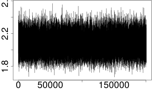
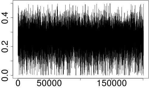
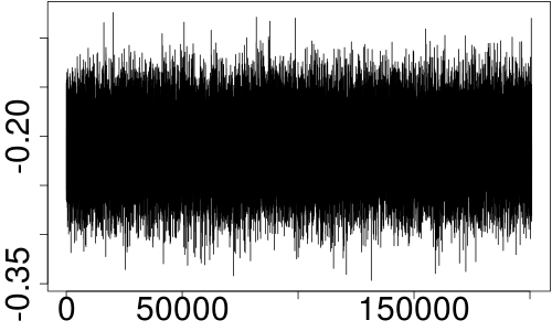
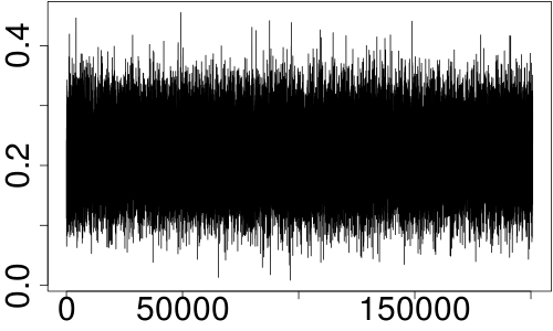
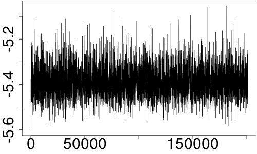
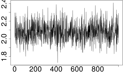
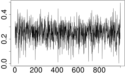
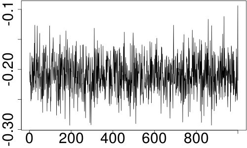
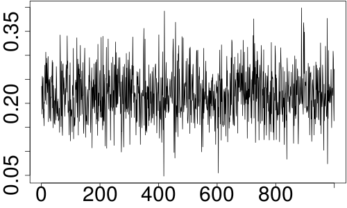
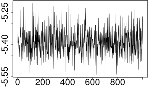
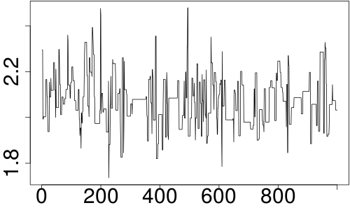
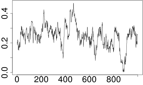
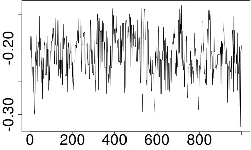
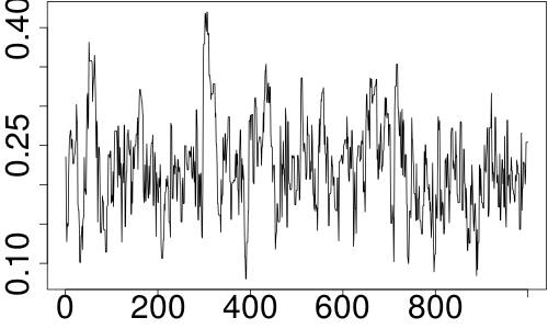
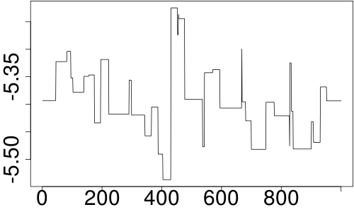
Figure 1: Original chain with sample size 200801 (top row). Thinned chain with sample size 1000 and thinning parameter equal to 200 (middle row). Unthinned chain with sample size 1000 (bottom row). For the middle and bottom rows the burn-in size is equal to 1000. The true parameter values of the FIEGARCH$(0,d,0)$ model corresponding to these graphs are $\nu_{0}=1.9$, $d_{0}=0.25$, $\theta_{0}=-0.15$, $\gamma_{0}=0.24$ and $\omega_{0}=-5.4$.

$\nu$	$d$	$\theta$	$\gamma$	$\omega$

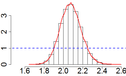
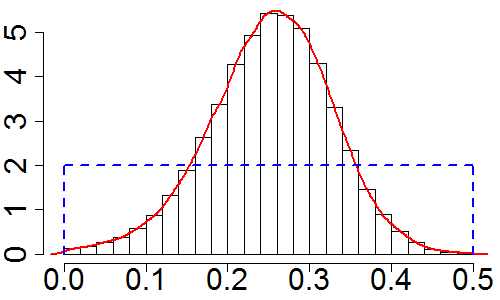
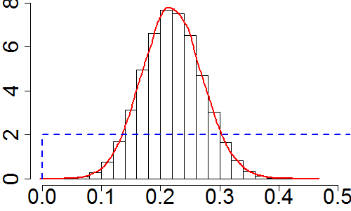
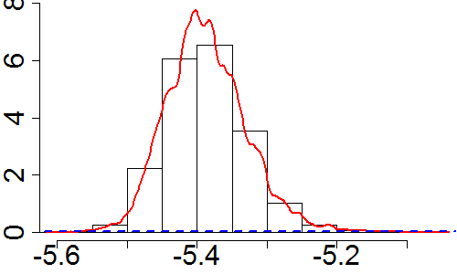
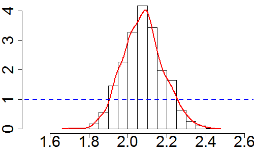
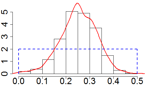
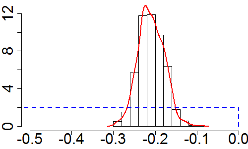
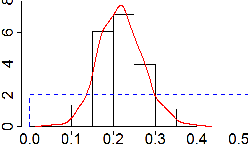
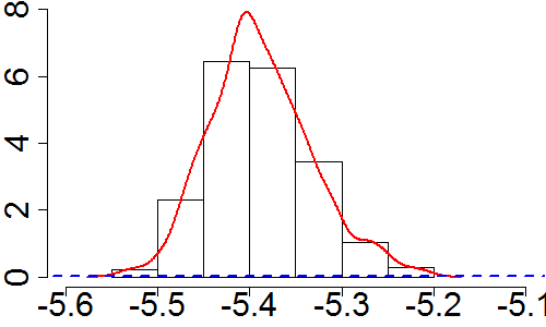
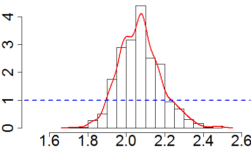
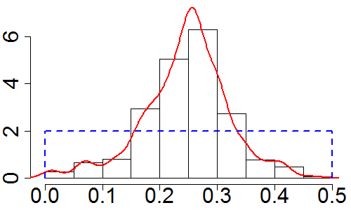
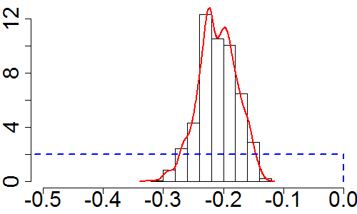
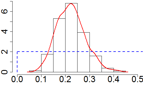
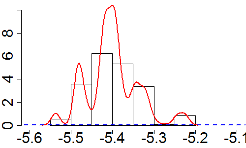
Figure 2: Histogram and kernel density functions for the original chain with sample size 200801 (top row); the thinned chain with sample size 1000 and thinning parameter equal to 200 (middle row) and the unthinned chain with sample size 1000 (bottom row). For the middle and bottom rows the burn-in size is equal to 1000. The dashed lines correspond to the graphs of the priors $\pi_{i}(\eta_{i})$ defined in (13), for $i\in\{1,\cdots,5\}$. The range for the $x$-axis was restricted to the intervals $[-1.5,2.5]$, $[-0.5,0]$, $[0,0.5]$ and $[-5.6,-5.1]$, respectively, for the parameters $\nu,\theta,\gamma$ and $\omega$. The true parameter values of the FIEGARCH$(0,d,0)$ model corresponding to these graphs are $\nu_{0}=1.9$, $d_{0}=0.25$, $\theta_{0}=-0.15$, $\gamma_{0}=0.24$ and $\omega_{0}=-5.4$.

As shown in Figure 1 (see also Table 1), the mean of the posterior distribution does not change significantly when the entire sample or the thinned chain is considered instead of the unthinned one. On the other hand, Figure 2 reinforces the idea that the entire chain gives better estimates for the density function (notice that the curves in the graphs are smoother). Although the thinned chain is not as efficient as the entire chain, it still provides better estimates for the density function than the unthinned one.

Table 1 presents the summary statistics for the samples obtained from the posterior distribution for each parameter of the FIEGARCH$(0,d,0)$ model. This table considers the entire, thinned and unthinned chains. The statistics reported in this table are the sample mean ($\bar{\eta}_{i}$), the sample standard deviation ($\mbox{sd}_{\eta_{i}}$) and the 95% credibility interval $CI_{0.95}(\eta_{i})$ for the parameter $\eta_{i}$ in $\boldsymbol{\eta}=(\nu,d,\theta,\gamma,\omega)^{\prime}:=(\eta_{1},\cdots,\eta_{5})^{\prime}$, for each $i\in\{1,\cdots,5\}$. The true parameter values considered for this illustration are $\nu_{0}\in\{1.1,1.5,2.5,5.0\}$, $d_{0}=0.25$, $\theta_{0}=-0.15$, $\gamma_{0}=0.24$ and $\omega_{0}=-5.4$.

Table 1: Summary for the entire, thinned (thinning parameter $\mathfrak{t}=200$) and unthinned sample from posterior distributions considering all prior uniforms: mean $\bar{\eta}_{i}$, standard deviation $\mbox{sd}_{\eta_{i}}$ and the 95% credibility interval $CI_{0.95}(\eta_{i})$ for the parameter $\eta_{i}$ in $\boldsymbol{\eta}=(\nu,d,\theta,\gamma,\omega)^{\prime}:=(\eta_{1},\cdots,\eta_{5})^{\prime}$, for each $i\in\{1,\cdots,5\}$. The true parameter values considered in this simulation are $\nu_{0}\in\{1.1,1.5,2.5,5.0\}$, $d_{0}=0.25$, $\theta_{0}=-0.15$, $\gamma_{0}=-0.24$ and $\omega_{0}=-5.4$. For the thinned and unthinned samples, the burn-in size is $\mathfrak{b}=1000$.

Chain	$\nu_{0}$		$\bar{\nu}$ $(\mbox{sd}_{\nu})$		$\bar{d}$ $(\mbox{sd}_{d})$		$\bar{\theta}$ $(\mbox{sd}_{\theta})$		$\bar{\gamma}$ $(\mbox{sd}_{\gamma})$		$\bar{\omega}$ $(\mbox{sd}_{\omega})$
			$CI_{0.95}(\nu)$		$CI_{0.95}(d)$		$CI_{0.95}(\theta)$		$CI_{0.95}(\gamma)$		$CI_{0.95}(\omega)$
Entire	1.1		1.095 (0.047)		0.263 (0.112)		-0.087 (0.038)		0.233 (0.062)		-5.469 (0.078)
			[1.006; 1.188]		[0.035; 0.464]		[-0.164; -0.016]		[0.114; 0.358]		[-5.612; -5.299]
	1.5		1.478 (0.067)		0.220 (0.081)		-0.184 (0.037)		0.240 (0.057)		-5.408 (0.058)
			[1.351; 1.612]		[0.056; 0.375]		[-0.257; -0.111]		[0.130; 0.355]		[-5.520; -5.291]
	1.9		2.077 (0.107)		0.252 (0.075)		-0.209 (0.032)		0.220 (0.051)		-5.386 (0.058)
			[1.874; 2.297]		[0.092; 0.392]		[-0.272; -0.148]		[0.122; 0.322]		[-5.487; -5.261]
	2.5		2.727 (0.153)		0.298 (0.056)		-0.203 (0.025)		0.205 (0.045)		-5.361 (0.053)
			[2.441; 3.040]		[0.184; 0.405]		[-0.253; -0.153]		[0.118; 0.296]		[-5.463; -5.252]
	5.0		5.227 (0.366)		0.220 (0.051)		-0.173 (0.019)		0.294 (0.036)		-5.303 (0.039)
			[4.548; 5.978]		[0.115; 0.317]		[-0.211; -0.135]		[0.224; 0.366]		[-5.384; -5.230]
Thinned	1.1		1.095 (0.047)		0.264 (0.110)		-0.087 (0.038)		0.233 (0.062)		-5.469 (0.080)
			[1.006; 1.193]		[0.038; 0.462]		[-0.161; -0.015]		[0.116; 0.362]		[-5.609; -5.288]
	1.5		1.480 (0.067)		0.221 (0.077)		-0.184 (0.037)		0.240 (0.057)		-5.405 (0.060)
			[1.353; 1.613]		[0.070; 0.367]		[-0.257; -0.104]		[0.129; 0.352]		[-5.524; -5.291]
	1.9		2.079 (0.103)		0.253 (0.075)		-0.210 (0.031)		0.218 (0.052)		-5.388 (0.056)
			[1.888; 2.292]		[0.098; 0.387]		[-0.269; -0.152]		[0.120; 0.327]		[-5.486; -5.261]
	2.5		2.718 (0.154)		0.298 (0.058)		-0.202 (0.026)		0.205 (0.044)		-5.361 (0.053)
			[2.427; 3.064]		[0.181; 0.410]		[-0.255; -0.153]		[0.121; 0.291]		[-5.466; -5.254]
	5.0		5.224 (0.363)		0.218 (0.052)		-0.173 (0.019)		0.295 (0.037)		-5.302 (0.039)
			[4.534; 5.991]		[0.112; 0.316]		[-0.211; -0.137]		[0.224; 0.370]		[-5.391; -5.230]
Unthinned	1.1		1.108 (0.039)		0.265 (0.129)		-0.089 (0.038)		0.230 (0.060)		-5.476 (0.052)
			[1.028; 1.198]		[0.016; 0.467]		[-0.176; -0.019]		[0.108; 0.345]		[-5.553; -5.366]
	1.5		1.474 (0.067)		0.250 (0.071)		-0.175 (0.035)		0.240 (0.053)		-5.426 (0.057)
			[1.352; 1.644]		[0.123; 0.393]		[-0.248; -0.100]		[0.135; 0.353]		[-5.535; -5.344]
	1.9		2.072 (0.109)		0.245 (0.074)		-0.210 (0.032)		0.223 (0.059)		-5.400 (0.062)
			[1.885; 2.303]		[0.068; 0.400]		[-0.273; -0.152]		[0.116; 0.349]		[-5.537; -5.244]
	2.5		2.720 (0.148)		0.308 (0.060)		-0.200 (0.026)		0.198 (0.042)		-5.367 (0.058)
			[2.412; 3.016]		[0.192; 0.426]		[-0.257; -0.155]		[0.119; 0.281]		[-5.462; -5.274]
	5.0		5.311 (0.356)		0.226 (0.045)		-0.176 (0.019)		0.293 (0.036)		-5.291 (0.035)
			[4.676; 6.070]		[0.137; 0.316]		[-0.215; -0.140]		[0.225; 0.368]		[-5.346; -5.246]

From Table 1 it is clear that, for any $\eta_{i}$, with $i\in\{1,\cdots,5\}$, the use of the entire or the thinned (thinning parameter $\mathfrak{t}=200$) does not yield significant improvement in terms of parameter estimation. Not even the differences in the sample standard deviations or in the credibility intervals, which are the statistics affected by the sample correlation, justify the computational effort to obtain a sample of size 200,801. The same conclusions are obtained when considering $d_{0}\in\{0.10,0.35,0.45\}$. This concludes the example.

Different prior distributions are tested as explained in the sequel. Since the conditional probability density function of $I_{0}$ given $\boldsymbol{\eta}$ is difficult to obtain, in all scenarios, it is assumed that $g(Z_{s})=0$, for all $s\leq 1$, and it is fixed $p_{\mbox{\tiny$I_{0}$}}(\cdot|\boldsymbol{\eta})=1$. Moreover, since (9) is well defined regardless the relation among the parameters of the model, it is assumed that

$$p_{\mbox{\tiny$(-i)$}}(\boldsymbol{\eta}_{(-i)}|\eta_{i})\propto\prod_{j\neq i}\pi_{j}(\eta_{j}),\quad\mbox{for any }i\in\{1,\cdots,5\}.$$

In a first moment the prior distributions for $\nu,d,\theta,\gamma$ and $\omega$ are selected by considering only the basic set of information usually available in practice. The information on each parameter and the corresponding prior selected are given in Table 2. This scenario shall be referred to as Case 1. Table 3 presents the mean, standard deviation, lower and upper limits for the transition kernel considered at iteration $m$ of the Gibbs sampler with Metropolis steps, when the prior for $\eta_{i}$ in $\boldsymbol{\eta}=(\nu,d,\theta,\gamma,\omega)^{\prime}:=(\eta_{1},\cdots,\eta_{5})^{\prime}$, for each $i\in\{1,\cdots,5\}$, is defined according to Case 1.

Table 2: Information available in practice for the parameter $\eta_{i}$ in $\boldsymbol{\eta}=(\nu,d,\theta,\gamma,\omega)^{\prime}:=(\eta_{1},\cdots,\eta_{5})^{\prime}$ and the corresponding prior considered, for each $i\in\{1,\cdots,5\}$.

Information Available		Prior
The generalized error distribution is well defined for any $\nu>0$.		$\nu\sim\mathds{I}_{(0,\infty)}(\nu)$ *
Long-memory in volatility is observed if and only if $d\in(0,0.5)$. This characteristic can be detected, for example, through the periodogram function of the time series $\{\ln(X_{t}^{2})\}_{t=1}^{n}$ (see Lopes and Prass, 2013).		$d\sim\mathcal{U}(0,0.5)$
Empirical evidence suggests that $\theta\in[-1,0]$. **		$\theta\sim\mathcal{U}(-1,0)$
Empirical evidence suggests that $\gamma\in[0,1]$. **		$\gamma\sim\mathcal{U}(0,1)$
$\omega=\mathds{E}(\ln(h_{t}^{2}))=\mathds{E}(\ln(X_{t}^{2}))+\mathds{E}(\ln(Z_{t}^{2}))$. The choice of the interval for $\omega$ will depend on the magnitude of the data. The sample mean of $\{\ln(X_{t}^{2})\}_{t=1}^{n}$ or $\ln(\hat{\sigma}_{X}^{2})$, where $\hat{\sigma}_{X}^{2}$ is the sample variance of $\{X_{t}\}_{t=1}^{n}$, can be used to obtain a rough approximation for $\omega$		$\omega\sim\mathcal{U}(-15,15)$.

Notes:

* Given $A\subset\mathds{R}$, the symbol $\mathds{I}_{A}(x)$ denotes the improper prior defined as $1$, if $x\in A$, and 0, if $x\notin A$.
** See, for instance, Nelson (1991); Bollerslev and Mikkelsen (1996); Ruiz and Veiga (2008); Lopes and Prass (2013). To the best of our knowledge, a FIEGARCH model for which $\theta$ or $\gamma$ are not in the intervals, respectively, $[-1,0]$ and $[0,1]$ has never been reported in the literature.

Table 3: Parameters of the truncated normal distribution (transition kernel) considered, at iteration $m$ of the Gibbs sampler, to obtain the sample from the posterior distribution of the parameter $\eta_{i}$ in $\boldsymbol{\eta}=(\nu,d,\theta,\gamma,\omega)^{\prime}:=(\eta_{1},\cdots,\eta_{5})^{\prime}$, for each $i\in\{1,\cdots,5\}$.

Parameter	$\nu$	$d$	$\theta$	$\gamma$	$\omega$
Mean ($y$)	$\nu^{(m-1)}$	$d^{(m-1)}$	$\theta^{(m-1)}$	$\gamma^{(m-1)}$	$\omega^{(m-1)}$
Standard Deviation ($\sigma$)	$0.500$	$0.025$	$0.050$	$0.050$	$1.500$
Lower Limit ($a$)	$\phantom{-}0.000$	$0.000$	$-1.000$	$0.000$	$-15.000$
Upper Limit ($b$)	$10.000$	$0.500$	$0.000$	$1.000$	$15.000$

Note:

$\eta_{i}^{(m-1)}$, for any $i\in\{1,\cdots,5\}$, denotes the parameter value obtained in the $(m-1)$th iteration. Different combinations of standard deviation, lower and upper limits were tested for the parameter $\eta_{i}$ in $\boldsymbol{\eta}=(\nu,d,\theta,\gamma,\omega)^{\prime}$, for each $i\in\{1,\cdots,5\}$. The values presented here correspond to the final choice.

In a second moment the knowledge on the true parameter values is gradually incorporated to provide more informative priors for $d,\theta$ and/or $\gamma$. This analysis, combined with the first scenario, provides information on the sensitivity of the estimates with respect to the priors functions and hyperparameters. In all cases, the priors for $\nu$ and $\omega$ are the same and are the ones defined in Table 2. The scenarios considered in this second step are described in the following and shall be referred to as Case 2 - Case 5.

Case 2: Gaussian Prior for $x=\phi^{-1}(d)$ and Uniform Priors for $\theta$ and $\gamma$.

In this case $\theta$ and $\gamma$ remain with the same priors as in Case 1. For the parameter $d$ it is assumed that $x\sim\mathcal{N}(\mu_{\phi},\sigma_{\phi}^{2})$ and $d=\phi(x)$, where $\phi:\mathbb{R}\to(0,0.5)$ is given by

$$\phi(x)=\frac{e^{x}}{2(1+e^{x})},\quad\mbox{for all }x\in\mathds{R}.$$ (14)

First, the knowledge of $d_{0}$ is applied to set $\mu_{\phi}=\phi^{-1}(d_{0})$, so $\mu_{\phi}\in\{-1.386,0.000,0.847,2.197\}$, respectively, for $d_{0}\in\{0.10,0.25,0.35,0.45\}$. This scenario shall be referred to as C2.1. Second, the knowledge on $d_{0}$ is ignored and the parameter $\mu_{\phi}$ is assumed to be equal to zero. This scenario shall be referred to as C2.2. For both, C2.1 and C2.2, different values of $\sigma_{\phi}$ are tested. Third, the approaches considered in C2.1 and C2.2 are combined by setting $\mu_{\phi}=\phi^{-1}(\bar{d})$, where $\bar{d}$ is the estimate of $d$ obtained in C2.2. This scenario shall be referred to as C2.3. The value of $\sigma_{\phi}$ considered in C2.3 is the one which provides better estimates for $d$ in C2.1.

The kernel parameter values for $\nu,\theta,\gamma$ and $\omega$ are the same as in the Case 1. For $x=\phi^{-1}(d)$, at iteration $m$ of the Gibbs sampler, the kernels mean ($y$), standard deviation ($sd$), lower ($a$) and upper limits ($b$) are set, respectively, as $x^{(m-1)}$, 1, -10 and 10, where $x^{(m-1)}$ is the parameter value obtained at iteration $m-1$.

Case 3: Gaussian Prior for $x=\phi^{-1}(d)$, Beta Prior for $-\theta$ and Uniform Prior for $\gamma$.

In this case, the priors of $\gamma$ and $d$ are the same ones considered, respectively, in Case 1 and in scenario C2.1 of Case 2. It is also assumed that $-\theta\sim\mbox{Beta}(a_{1},b_{1})$, which is equivalent to set

$$\pi_{3}(\theta)=(-\theta)^{a_{1}-1}(1+\theta)^{b_{1}-1}B(a_{1},b_{1}),\quad\theta\in[-1,0],$$

where $B(\cdot,\cdot)$ is the beta function.

First, the fact that $X\sim\mbox{Beta}(a,b)$ implies $\mathbb{E}(X)=a(a+b)^{-1}$, is applied to set $b_{1}=a_{1}(1+\theta_{0})(-\theta_{0})^{-1}$, where $\theta_{0}=-0.15$ is the true parameter value considered in this simulation study. Different values of $a_{1}$ are tested. This scenario shall be referred to as C3.1. Second, the knowledge on $\theta_{0}$ is ignored and different combinations of $a_{1}$ and $b_{1}$ are tested. This scenario shall be referred to as C3.2. Third, the approaches considered in C3.1 and C3.2 are combined by setting $b_{1}=a_{1}(1+\bar{\theta}_{0})(-\bar{\theta}_{0})^{-1}$, where $-\bar{\theta}_{0}$ is the estimate of $\theta$ obtained in C3.2. The value of $a_{1}$ considered in this case is the one which provides better estimates for $\theta$ in C3.1. This scenario shall be referred to as C3.3.

The kernel parameter values are the same as in Case 2.

Case 4: Gaussian Prior for $x=\phi^{-1}(d)$, Beta Priors for $-\theta$ and $\gamma$.

In this case, the priors of $d$ and $-\theta$ are the same ones considered, respectively, in scenario C2.1 of Case 2 and in scenario C3.1 of Case 3. It is also assumed that $\gamma\sim\mbox{Beta}(a_{2},b_{2})$. Two scenarios, denoted by C4.1 and C4.2 are considered. With the obvious identifications, the construction of C4.1 and C4.2 is analogous, respectively, to the construction of scenarios C3.1 and C3.2 in Case 3.

The kernel parameter values are the same as in Case 2.

Case 5: Beta Priors for $2d$, $-\theta$ and $\gamma$.

In this case, the priors of $-\theta$ and $\gamma$ are the same ones considered, respectively, in scenario C3.1 of Case 3 and in scenario C4.1 of Case 4. Moreover, for each $d_{0}\in\{0.10,0.25,0.35,0.45\}$ considered in this simulation study, it is assumed that $2d\sim\mbox{Beta}(a_{3},b_{3})$, which is equivalent to set

$$\pi_{2}(d)=2(2d)^{a_{3}-1}(1-2d)^{b_{3}-1}B(a_{3},b_{3}),\quad d\in[0,0.5],$$

where $B(\cdot,\cdot)$ is the beta function.

In this case, only two scenarios are considered. First, it is assumed that $b_{3}=a_{3}(1-2d_{0})(2d_{0})^{-1}$ and different values of $a_{3}$ are tested. This scenario shall be referred to as C5.1. Second, an approach similar to scenarios C3.3 and C4.3, respectively, in Case 3 and Case 4, is considered. However, in this case, it is assumed that $b_{3}=a_{3}(1-2\bar{d})(2\bar{d})^{-1}$, with $\bar{d}$ obtained in Case 1. The value of $a_{3}$ considered in this case is the one which provides better estimates for $d$ in C5.1. This scenario shall be referred to as C5.2.

The kernel parameter values are the same as in Case 1.

4.3 Estimates and Performance Measures

Let $\{\eta_{i}^{(k)}\}_{k=1}^{M}$ be a sample of size $M$ from the posteriori distribution of $\eta_{i}$ in $\boldsymbol{\eta}=(\nu,d,\theta,\gamma,\omega)^{\prime}:=(\eta_{1},\cdots,\eta_{5})^{\prime}$, for any $i\in\{1,\cdots,5\}$. Denote by $\bar{\eta}_{i}$ and $\mbox{sd}_{\eta_{i}}$, respectively, the sample mean and standard deviation of $\{\eta_{i}^{(k)}\}_{k=1}^{M}$, namely,

$$\bar{\eta}_{i}=\frac{1}{M}\sum_{k=1}^{M}\eta_{i}^{(k)}\quad\mbox{and}\quad\mbox{sd}_{\eta_{i}}=\sqrt{\frac{1}{M}\sum_{k=1}^{M}(\eta_{i}^{(k)}-\bar{\eta}_{i})^{2}},\quad\mbox{for any}\quad i\in\{1,\cdots,5\}.$$

Then the estimate $\hat{\eta}_{i}$ of $\eta_{i}$ is defined as $\hat{\eta}_{i}:=\bar{\eta}_{i}$.

Moreover, let $\hat{q}_{i}(\alpha)$ denote the $\alpha$ quantile for the posterior sample distribution of $\eta_{i}$, for any $\alpha\in[0,1]$ and $i\in\{1,\cdots,5\}$. Then a $100(1-\alpha)\%$ credibility interval for $\eta_{i}$ is given by

$$CI_{1-\alpha}(\eta_{i})=\Big{[}\hat{q}_{i}\Big{(}\frac{\alpha}{2}\Big{)},\hat{q}_{i}\Big{(}\frac{1-\alpha}{2}\Big{)}\Big{]},\quad\mbox{for any}\quad i\in\{1,\cdots,5\}.$$

Furthermore, the estimation bias and the absolute percentage error (ape) of estimation are given, respectively, by

$$\mbox{bias}_{\eta_{i}}=\bar{\eta}_{i}-\eta_{i}\quad\mbox{and}\quad\mbox{ape}_{\eta_{i}}=\bigg{|}\frac{\mbox{bias}_{\eta_{i}}}{\eta_{i}}\bigg{|},\quad\mbox{for any}\quad i\in\{1,\cdots,5\}.$$

4.4 Results

The results obtained in this simulation study, by considering the scenarios described in Section 4.2, are the following.

Case 1: The Priors as Defined in Table 2.

Table 4 present the summary statistics for the samples obtained from the posterior distribution for each parameter of the FIEGARCH$(0,d,0)$ model. The statistics reported in this table (the same applies to Table 5) are the sample mean ($\bar{\eta}_{i}$), the sample standard deviation ($\mbox{sd}_{\eta_{i}}$) and the 95% credibility interval $CI_{0.95}(\eta_{i})$ for the parameter $\eta_{i}$ in $\boldsymbol{\eta}=(\nu,d,\theta,\gamma,\omega)^{\prime}:=(\eta_{1},\cdots,\eta_{5})^{\prime}$, for each $i\in\{1,\cdots,5\}$. The bold-face font for the mean indicates that the absolute percentage error of estimation ($\mbox{ape}_{\eta_{i}}$) in the corresponding case is higher than 0.10 (that is, 10%). The bold-face font for the credibility interval indicates that the true parameter value is not contained in the interval.

Table 4: Summary for the sample obtained from posterior distributions considering all prior uniforms: mean $\bar{\eta}_{i}$, standard deviation $\mbox{sd}_{\eta_{i}}$ and the 95% credibility interval $CI_{0.95}(\eta_{i})$ for the parameter $\eta_{i}$ in $\boldsymbol{\eta}=(\nu,d,\theta,\gamma,\omega)^{\prime}:=(\eta_{1},\cdots,\eta_{5})^{\prime}$, for each $i\in\{1,\cdots,5\}$. The true parameter values considered in this simulation are $d_{0}\in\{0.10,0.25,0.35,0.45\}$, $\nu_{0}\in\{1.1,1.5,2.5,5.0\}$, $\theta_{0}=-0.15$, $\gamma_{0}=-0.24$ and $\omega_{0}=-5.4$.

$d_{0}$	$\nu_{0}$		$\bar{\nu}$ $(\mbox{sd}_{\nu})$		$\bar{d}$ $(\mbox{sd}_{d})$		$\bar{\theta}$ $(\mbox{sd}_{\theta})$		$\bar{\gamma}$ $(\mbox{sd}_{\gamma})$		$\bar{\omega}$ $(\mbox{sd}_{\omega})$
			$CI_{0.95}(\nu)$		$CI_{0.95}(d)$		$CI_{0.95}(\theta)$		$CI_{0.95}(\gamma)$		$CI_{0.95}(\omega)$
0.10	1.1		1.093 (0.044)		0.181 (0.123)		-0.084 (0.041)		0.236 (0.066)		-5.438 (0.058)
			[0.989; 1.195]		[0.005; 0.458]		[-0.171; -0.013]		[0.093; 0.357]		[-5.551; -5.337]
	1.5		1.480 (0.069)		0.147 (0.079)		-0.177 (0.038)		0.232 (0.052)		-5.420 (0.036)
			[1.353; 1.635]		[0.020; 0.330]		[-0.258; -0.106]		[0.122; 0.340]		[-5.510; -5.338]
	1.9		2.088 (0.111)		0.093 (0.055)		-0.220 (0.032)		0.216 (0.060)		-5.410 (0.035)
			[1.908; 2.296]		[0.004; 0.201]		[-0.286; -0.154]		[0.105; 0.337]		[-5.486; -5.340]
	2.5		2.724 (0.140)		0.192 (0.076)		-0.201 (0.025)		0.198 (0.045)		-5.388 (0.031)
			[2.491; 3.027]		[0.038; 0.330]		[-0.256; -0.153]		[0.116; 0.287]		[-5.448; -5.333]
	5.0		5.297 (0.364)		0.101 (0.051)		-0.174 (0.020)		0.297 (0.036)		-5.336 (0.028)
			[4.641; 6.014]		[0.015; 0.217]		[-0.215; -0.133]		[0.232; 0.374]		[-5.383; -5.287]
0.25	1.1		1.108 (0.039)		0.265 (0.129)		-0.089 (0.038)		0.230 (0.060)		-5.476 (0.052)
			[1.028; 1.198]		[0.016; 0.467]		[-0.176; -0.019]		[0.108; 0.345]		[-5.553; -5.366]
	1.5		1.474 (0.067)		0.250 (0.071)		-0.175 (0.035)		0.240 (0.053)		-5.426 (0.057)
			[1.352; 1.644]		[0.123; 0.393]		[-0.248; -0.100]		[0.135; 0.353]		[-5.535; -5.344]
	1.9		2.072 (0.109)		0.245 (0.074)		-0.210 (0.032)		0.223 (0.059)		-5.400 (0.062)
			[1.885; 2.303]		[0.068; 0.400]		[-0.273; -0.152]		[0.116; 0.349]		[-5.537; -5.244]
	2.5		2.720 (0.148)		0.308 (0.060)		-0.200 (0.026)		0.198 (0.042)		-5.367 (0.058)
			[2.412; 3.016]		[0.192; 0.426]		[-0.257; -0.155]		[0.119; 0.281]		[-5.462; -5.274]
	5.0		5.311 (0.356)		0.226 (0.045)		-0.176 (0.019)		0.293 (0.036)		-5.291 (0.035)
			[4.676; 6.070]		[0.137; 0.316]		[-0.215; -0.140]		[0.225; 0.368]		[-5.346; -5.246]
0.35	1.1		1.099 (0.040)		0.349 (0.108)		-0.097 (0.038)		0.230 (0.056)		-5.495 (0.090)
			[1.009; 1.194]		[0.093; 0.492]		[-0.178; -0.027]		[0.121; 0.330]		[-5.674; -5.318]
	1.5		1.479 (0.065)		0.329 (0.065)		-0.178 (0.036)		0.246 (0.052)		-5.423 (0.076)
			[1.352; 1.639]		[0.204; 0.461]		[-0.246; -0.106]		[0.143; 0.340]		[-5.561; -5.302]
	1.9		2.064 (0.110)		0.364 (0.054)		-0.199 (0.030)		0.233 (0.050)		-5.377 (0.090)
			[1.843; 2.299]		[0.227; 0.461]		[-0.265; -0.139]		[0.139; 0.330]		[-5.535; -5.199]
	2.5		2.732 (0.150)		0.380 (0.052)		-0.201 (0.024)		0.200 (0.043)		-5.307 (0.066)
			[2.481; 3.031]		[0.283; 0.479]		[-0.254; -0.161]		[0.110; 0.285]		[-5.410; -5.149]
	5.0		5.229 (0.321)		0.318 (0.040)		-0.177 (0.019)		0.289 (0.036)		-5.227 (0.046)
			[4.603; 5.864]		[0.243; 0.409]		[-0.216; -0.140]		[0.227; 0.366]		[-5.298; -5.127]
0.45	1.1		1.096 (0.039)		0.436 (0.053)		-0.115 (0.034)		0.241 (0.054)		-5.453 (0.128)
			[1.010; 1.161]		[0.313; 0.499]		[-0.187; -0.047]		[0.136; 0.338]		[-5.716; -5.174]
	1.5		1.475 (0.073)		0.411 (0.048)		-0.179 (0.034)		0.257 (0.048)		-5.411 (0.123)
			[1.353; 1.627]		[0.311; 0.494]		[-0.246; -0.110]		[0.158; 0.353]		[-5.600; -5.133]
	1.9		2.052 (0.111)		0.450 (0.032)		-0.191 (0.026)		0.243 (0.043)		-5.367 (0.130)
			[1.846; 2.279]		[0.385; 0.497]		[-0.238; -0.141]		[0.165; 0.320]		[-5.614; -5.125]
	2.5		2.725 (0.152)		0.447 (0.032)		-0.206 (0.021)		0.211 (0.041)		-5.150 (0.081)
			[2.461; 3.021]		[0.381; 0.495]		[-0.247; -0.167]		[0.133; 0.296]		[-5.310; -4.985]
	5.0		5.177 (0.322)		0.417 (0.032)		-0.177 (0.019)		0.286 (0.032)		-5.041 (0.068)
			[4.553; 5.832]		[0.348; 0.480]		[-0.220; -0.140]		[0.228; 0.350]		[-5.182; -4.929]

Note:

The bold-face font for the estimated mean indicates that the absolute percentage error is higher than 10%. The bold-face font for the credibility interval indicates that the interval does not contain the true parameter value.

From Table 4 one observes that the parameters $\nu$ and $\omega$ are always well estimated, in terms of absolute percentage error (ape), regardless the combination of $d_{0}\in\{0.10,0.25,0.35,0.45\}$ and $\nu_{0}\in\{1.1,1.5,2.5,5.0\}$ considered (the error is less than 10% in all cases). The credibility interval $CI_{0.95}(\nu)$ contains the true parameter value $\nu_{0}$ in all cases, except when $d_{0}=0.10$ and $\nu_{0}=1.9$. Also, the estimation bias for $\nu$ is always negative when $\nu_{0}<1.9$ and positive when $\nu_{0}\geq 1.9$, except for the combination $(\nu_{0},d_{0})=(1.1,0.25)$. For the parameter $\omega$, the credibility interval $CI_{0.95}(\omega)$ does not contain the true parameter value ($\omega_{0}=-5.4$) in 5 out of 20 combinations of $\nu_{0}$ and $d_{0}$ (see $\nu_{0}=5$ and all $d_{0}$; $\nu_{0}=2.5$ and $d_{0}=0.45$). Moreover, the estimation bias for $\omega$ is always negative when $\nu_{0}\leq 1.5$ and always positive when $\nu_{0}\geq 2.5$.

Table 4 also reports that $\mbox{ape}_{\theta}>10\%$ for all combinations of $d_{0}$ and $\nu_{0}$. On the other hand, in most cases (14 out of 20), the credibility interval $CI_{0.95}(\theta)$ contains the true parameter value $\theta_{0}=-0.15$. The cases for which $\theta_{0}\notin CI_{0.95}(\theta)$ are $\nu=1.9$ and $d_{0}\in\{0.10,0.25\}$ and $\nu_{0}=2.5$ and any $d_{0}$. The bias for $\theta$ is always positive when $\nu_{0}=1.1$ (for any $d_{0}$) and negative in all other cases.

Furthermore, Table 4 shows that the parameter $\gamma$ seems to be better estimated when the GED distribution presents heavy tails ($\nu_{0}<2$), except when $d=0.10$, in which case $\mbox{ape}_{\gamma}>10\%$ when $\nu_{0}=1.9$. Also, with exception of four cases ($d_{0}=0.10$ and $\nu_{0}\in\{1.1,1.5,2.5\}$; $d_{0}=0.25$ and $\nu_{0}=2.5$), the parameter $d$ is always well estimated. The bias for parameters $d$ and $\gamma$ does not seem to follow any pattern and both, $d_{0}\in CI_{0.95}(d)$ and $\gamma_{0}\in CI_{0.95}(\gamma)$, for any combination of $\nu_{0}$ and $d_{0}$.

Case 2: Gaussian Prior for $x=\phi^{-1}(d)$ and Uniform Priors for $\theta$ and $\gamma$.

Changing the prior for $d$ does not yield significant difference on the estimation of $\nu$, $\theta$, $\gamma$ and $\omega$.

When the true value of $d_{0}$ is used to set $\mu_{\phi}=\phi^{-1}(d_{0})$ (scenario C2.1), the best performance is observed by letting $\sigma_{\phi}=0.15$. In this case, the absolute percentage error of estimation ($\mbox{ape}_{d}$) is smaller than 10% for all combinations of $\nu_{0}$ and $d_{0}$, with $d_{0}\in\{0.10,0.25,0.35,0.45\}$ and $\nu_{0}\in\{1.1,1.5,2.5,5.0\}$. If $\sigma_{\phi}=0.10$ the chain takes too long to move from the initial point when $d_{0}=0.10$. When $\sigma_{\phi}=0.25$, there is only one case for which $\mbox{ape}_{d}>10\%$ ($d_{0}=0.10$ and $\nu_{0}=2.5$). In fact, in this case, $\mbox{ape}_{d}=0.103$, which is still acceptable ($\sigma_{\phi}=0.15$ still seems to be the best choice). Furthermore, as $\sigma_{\phi}$ increases, the number of cases for which $\mbox{ape}_{d}>10\%$ also increases. For instance, when $\sigma_{\phi}\in\{0.50,1.00,3.00\}$, $\mbox{ape}_{d}>10\%$ in 2, 4 and 10 cases, respectively.

When $d_{0}$ is assumed unknown and $\mu_{\phi}$ is set to zero (scenario C2.2), $\sigma_{\phi}=3$ seems to provide better results than smaller values of $\sigma_{\phi}$. Under this scenario, $\mbox{ape}_{d}>10\%$ for 8 out of 20 combinations of $\nu_{0}$ and $d_{0}$. Therefore, $d\sim\mathcal{U}(0,0.5)$ still provides better estimates for the parameter $d$ (see Table 4). Higher values of $\sigma_{\phi}$ do not improve the estimation of $d$. Too high values of $\sigma_{\phi}$ actually make the estimation worst. In particular, when $\sigma_{\phi}=4$ the results are similar to $\sigma_{\phi}=3$, if $d_{0}>0.1$. If $d_{0}=0.1$ then $\sigma_{\phi}=3$ is slightly better than $\sigma_{\phi}=4$. When $\sigma_{\phi}=5$, $\mbox{ape}_{d}$ is, in most cases, higher than when $\sigma_{\phi}=3$. For $\sigma_{\phi}$ smaller than 3 the estimation bias is much higher. For instance, when $\sigma_{\phi}=0.15$, $\mbox{ape}_{d}\leq 10\%$ only for $d_{0}=0.25$ (for all $\nu_{0}$). For all other combinations of $d_{0}$ and $\nu_{0}$ $\mbox{ape}_{d}>20\%$. Also, when $b=1$, $\mbox{ape}_{d}>20\%$ in 12 out of 20 cases. In particular, $\mbox{ape}_{d}>20\%$ for $d_{0}=0.10$ and all $\nu_{0}$. As it should be expected, C2.1 performs much better than C2.2.

Upon considering a two step estimator (scenario C2.3), no improvement is observed, when compared to scenario C2.2. In fact, the estimates obtained by letting $\mu_{\phi}=\phi^{-1}(\bar{d})$ (where $\bar{d}$ is the estimate of $d$ obtained in C2.2) and $\sigma_{\phi}=0.15$ (the parameter which leads to the best performance in C2.1) are very close to $\bar{d}$ itself.

Case 3: Gaussian Prior for $x=\phi^{-1}(d)$, Beta Prior for $-\theta$ and Uniform Prior for $\gamma$.

The estimation of $\nu$, $d$, $\gamma$ and $\omega$ is not significantly affected by the change in the prior for $-\theta$.

When the knowledge on the true parameter values $d_{0}$ and $\theta_{0}$ is applied to set $\mu_{\phi}=\phi^{-1}(d_{0})$, $\sigma_{\phi}=0.15$, for each $d_{0}\in\{0.10,0.25,0.35,0.45\}$ (the best scenario in Case 2), and $b_{1}=a_{1}(1+\theta_{0})(-\theta_{0})^{-1}$ (scenario C3.1), it is observed that larger values of $a_{1}$ lead to better estimates for $\theta$. Although any $a_{1}\in\{110,150,200\}$ leads to $\mbox{ape}_{\theta}\leq 10\%$, for all combinations of $d_{0}\in\{0.10,0.25,0.35,0.45\}$ and $\nu_{0}\in\{1.1,1.5,2.5,5.0\}$, the best performance is obtained by setting $a_{1}=110$ ($b_{1}\approx 623.333$). As $a_{1}$ decreases, the estimation performance decreases. For instance, when $a_{1}=100$, one case for which $\mbox{ape}_{\theta}>10\%$ is observed. When $a_{1}=20$ the number of cases for which $\mbox{ape}_{\theta}>10\%$ increases to 10 and no case for which $\mbox{ape}_{\theta}\leq 10\%$ is observed if $a_{1}\in\{2.0,0.1\}$. More specifically, for any $a_{1}\in\{2.0,0.1\}$, $10\%<\mbox{ape}_{\theta}\leq 20\%$ for $\nu_{0}\in\{1.5,5.0\}$ and all values of $d_{0}$ (8 out of 20 cases) and, in the remaining 12 cases, $\mbox{ape}_{\theta}>20\%$.

By assuming $\theta_{0}$ unknown (scenario C3.2) or by considering a two step estimator (scenario C3.3), no case for which $\mbox{ape}_{\theta}<10\%$ is observed. The combinations of $a_{1}$ and $b_{1}$ tested in scenario C3.2 are: $(a_{1},b_{1})\in\{$(2, 3), (2, 5), (2, 9), (4, 7), (5, 7), (10, 40), (10, 60), (10, 70), (100, 500), (100, 600)$\}$. Among these values, the best performance is obtained when $a_{1}=10$ and $b_{1}=50$. In this case, $10\%<\mbox{ape}_{\theta}\leq 20\%$ in 12 out of 20 cases, which is slightly better than the performance obtained assuming $\theta\sim\mathcal{U}(0,1)$ (in this case, $10\%<\mbox{ape}_{\theta}\leq 20\%$ in 8 out of 20 cases).

Case 4: Gaussian Prior for $x=\phi^{-1}(d)$, Beta Priors for $-\theta$ and $\gamma$.

Analogously to Case 2 and Case 3, the estimation of $\nu$, $d$, $\theta$ and $\omega$ is not significantly affected by the change in the prior for $\gamma$.

By considering the true parameter values $d_{0}$, $\theta_{0}$ and $\gamma_{0}$ and setting $\mu_{\phi}=\phi^{-1}(d_{0})$, $\sigma_{\phi}=0.15$, for each $d_{0}\in\{0.10,0.25,0.35,0.45\}$ (the best scenario in Case 2), $a_{1}=110$, $b_{1}=a_{1}(1+\theta_{0})(-\theta_{0})^{-1}$ (the best scenario in Case 3) and $b_{2}=a_{2}(1-\gamma_{0})\gamma_{0}^{-1}$ (scenario C4.1), it is observed the following: larger values of $a_{2}$ (smaller than $a_{1}$, however) lead to better estimates for $\gamma$ and as $a_{2}$ decreases, the estimation performance decays. For instance, when $a_{2}=40$ only one case for which $\mbox{ape}_{\theta}>10\%$ is observed and when $a_{2}\in\{10,25,30\}$, the number of cases increases to 5 ($d_{0}=0.45$ and all $\nu_{0}$). On the other hand, any $a_{2}\in\{50,100\}$ gives $\mbox{ape}_{\theta}\leq 10\%$, for all combinations of $d_{0}\in\{0.10,0.25,0.35,0.45\}$ and $\nu_{0}\in\{1.1,1.5,2.5,5.0\}$. The simulation results for $a_{2}=50$ ($b_{2}\approx 158.333$) are illustrated in Figure 3.

Figure 3 shows the sample mean (solid circle) and the 95% credibility interval (solid line) for the sample obtained from the posterior distribution of $\nu,d,\theta,\gamma$ and $\omega$ (respectively, from top to bottom), for each combination of $d_{0}$ and $\nu_{0}$. The true parameter values $\nu_{0},d_{0},\theta_{0},\gamma_{0}$ and $\omega_{0}$ are represented in the corresponding row by the dashed line. The graphs related to $\theta,\gamma$ and $\omega$ (respectively, the third, fourth and fifth rows, from top to bottom) consider the same scale for all $d_{0}\in\{0.10,0.25,0.35,0.45\}$. Also, for the parameters $\theta,\gamma$ and $\omega$, there is one graph for each $d_{0}$ and, for each one of these graphs, the true value of $\nu_{0}$ is indicated in the $x$-axis.

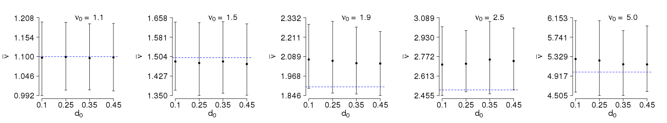
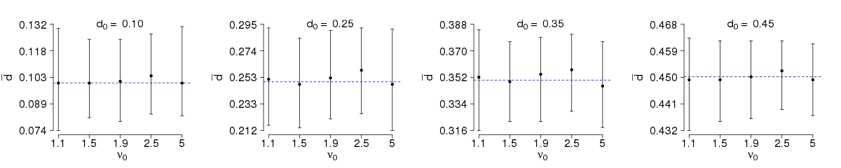
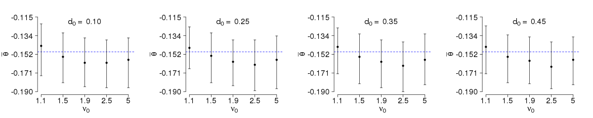
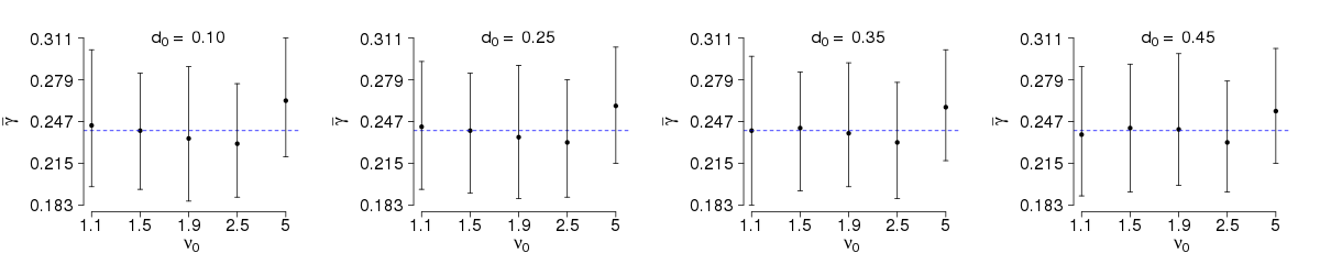
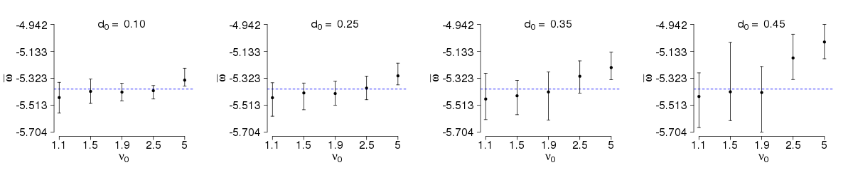
Figure 3: Posterior mean (solid circle), the true parameter value (dashed line) and the 95% credibility interval (solid line) for the parameters $\nu,d,\theta,\gamma$ and $\omega$ (from top to bottom), for each combination of $d_{0}$ and $\nu_{0}$. The posterior distributions were obtained by considering an improper prior for $\nu$, a Gaussian prior for $\phi^{-1}(d)$, Beta priors for $-\theta$ and $\gamma$ and a uniform prior for $\omega$. The true parameters values considered in this simulation are $d_{0}\in\{0.10,0.25,0.35,0.45\}$, $\nu_{0}\in\{1.1,1.5,2.5,5.0\}$, $\theta_{0}=-0.15$, $\gamma_{0}=-0.24$ and $\omega_{0}=-5.4$.

From Figure 3 one observes that, for $\nu$ and $\omega$, the conclusion regarding the estimation bias and the credibility intervals are basically the same as in Case 1 (see Table 4). On the other hand, under C4.1 of Case 4), $\mbox{ape}_{\eta_{i}}<10\%$, for all $i\in\{1,\cdots,5\}$ and any combination of $d_{0}\in\{0.10,0.25,0.35,0.45\}$ and $\nu_{0}\in\{1.1,1.5,2.5,5.0\}$ (compare the parameter $\theta$ in Table 4 and Figure 3). As in Case 1, the bias for $\theta$ is always positive when $\nu_{0}=1.1$ (for any $d_{0}$) and negative when $\nu_{0}>1.1$ and the bias for the parameters $d$ and $\gamma$ does not seem to follow any pattern. Under the current scenario, $d_{0},\theta_{0}$ and $\gamma_{0}$ are all contained in the respective credibility intervals, for any combination of $d_{0}\in\{0.10,0.25,0.35,0.45\}$ and $\nu_{0}\in\{1.1,1.5,2.5,5.0\}$.

When the true value of $\gamma_{0}$ is not used to choose $b_{2}$ (scenario C4.2) similar results to the ones in Figure 3 are still obtained for some combinations of $(a_{2},b_{2})$. Not surprisingly, the pairs $(a_{2},b_{2})$ which lead to good estimates are such that $a_{2}(a_{2}+b_{2})^{-1}$ (the mean $\mu_{B}$ of the prior distribution) is close to $\gamma_{0}$. For instance, when $(a_{2},b_{2})\in\{(100,300),(100,350)\}$ ($\mu_{B}$ is, respectively, equal to 0.25 and 0.22, while $\gamma_{0}=0.24$) it is obtained $\mbox{ape}_{\gamma}<10\%$ for all combinations of $d_{0}\in\{0.10,0.25,0.35,0.45\}$ and $\nu_{0}\in\{1.1,1.5,2.5,5.0\}$. The pair $(a_{2},b_{2})=(100,350)$ provides slightly better results than $(a_{2},b_{2})=(100,300)$ only when $\nu_{0}=5$. When $(a_{2},b_{2})=(100,280)$ (so $\mu_{B}\approx 0.26$), $\mbox{ape}_{\gamma}\leq 10\%$ in 16 out of 20 cases (in the remaining 4 cases, $\mbox{ape}_{\gamma}$ does not exceed 13.4%).

On the other hand, choosing $a_{2}$ and $b_{2}$ such that $a_{2}(a_{2}+b_{2})^{-1}$ is close to the true $\gamma_{0}$ does not necessarily lead to good estimates. For instance, if $(a_{2},b_{2})=(5,15)$ then $\mu_{B}=0.25$, as it is when $(a_{2},b_{2})=(100,300)$, but $\mbox{ape}_{\gamma}>10\%$ in 6 out of 20 cases. Also, it is not evident that the more distant $a_{2}(a_{2}+b_{2})^{-1}$ is from $\gamma_{0}$, the worst is the estimation. For instance, by letting $(a_{2},b_{2})\in\{(3,15),(100,440),(10,30),(10,40),(20,80),(100,400),(100,270),(5,10)\}$ then, respectively, $\mu_{B}\in\{0.167,0.185,0.200,0.200,0.200,0.200,0.270,0.330\}$ and it is observed that $\mbox{ape}_{\gamma}>10\%$ in 14, 20, 4, 10, 12, 16, 13 and 5 out of 20 cases, respectively.

Table 5: Summary for the sample obtained from posterior distributions considering Beta priors for $2d,-\theta$ and $\gamma$: mean $\bar{\eta}_{i}$, standard deviation $\mbox{sd}_{\eta_{i}}$ and the 95% credibility interval $CI_{0.95}(\eta_{i})$ for the parameter $\eta_{i}$ in $\boldsymbol{\eta}=(\nu,d,\theta,\gamma,\omega)^{\prime}:=(\eta_{1},\cdots,\eta_{5})^{\prime}$, for each $i\in\{1,\cdots,5\}$. The true parameter values considered in this simulation are $d_{0}\in\{0.10,0.25,0.35,0.45\}$, $\nu_{0}\in\{1.1,1.5,2.5,5.0\}$, $\theta_{0}=-0.15$, $\gamma_{0}=-0.24$ and $\omega_{0}=-5.4$.

$d_{0}$	$\nu_{0}$		$\bar{\nu}$ $(\mbox{sd}_{\nu})$		$\bar{d}$ $(\mbox{sd}_{d})$		$\bar{\theta}$ $(\mbox{sd}_{\theta})$		$\bar{\gamma}$ $(\mbox{sd}_{\gamma})$		$\bar{\omega}$ $(\mbox{sd}_{\omega})$
			$CI_{0.95}(\nu)$		$CI_{0.95}(d)$		$CI_{0.95}(\theta)$		$CI_{0.95}(\gamma)$		$CI_{0.95}(\omega)$
0.10	1.1		1.102 (0.045)		0.100 (0.018)		-0.144 (0.011)		0.243 (0.026)		-5.472 (0.063)
			[1.012; 1.198]		[0.069; 0.139]		[-0.170; -0.124]		[0.199; 0.294]		[-5.569; -5.347]
	1.5		1.483 (0.063)		0.102 (0.019)		-0.154 (0.013)		0.239 (0.024)		-5.412 (0.047)
			[1.364; 1.607]		[0.069; 0.141]		[-0.178; -0.132]		[0.190; 0.285]		[-5.524; -5.333]
	1.9		2.067 (0.108)		0.101 (0.016)		-0.160 (0.012)		0.234 (0.027)		-5.422 (0.034)
			[1.879; 2.309]		[0.070; 0.134]		[-0.186; -0.137]		[0.184; 0.291]		[-5.498; -5.360]
	2.5		2.702 (0.143)		0.106 (0.019)		-0.160 (0.012)		0.231 (0.023)		-5.407 (0.022)
			[2.442; 2.977]		[0.074; 0.150]		[-0.186; -0.136]		[0.187; 0.277]		[-5.470; -5.375]
	5.0		5.251 (0.391)		0.099 (0.017)		-0.158 (0.012)		0.263 (0.024)		-5.343 (0.036)
			[4.514; 6.080]		[0.070; 0.132]		[-0.186; -0.134]		[0.220; 0.312]		[-5.390; -5.265]
0.25	1.1		1.095 (0.044)		0.255 (0.031)		-0.145 (0.012)		0.242 (0.028)		-5.455 (0.057)
			[0.986; 1.190]		[0.197; 0.315]		[-0.173; -0.123]		[0.191; 0.295]		[-5.559; -5.348]
	1.5		1.485 (0.066)		0.252 (0.030)		-0.154 (0.013)		0.240 (0.022)		-5.421 (0.046)
			[1.357; 1.628]		[0.193; 0.313]		[-0.180; -0.132]		[0.195; 0.281]		[-5.529; -5.324]
	1.9		2.058 (0.113)		0.260 (0.030)		-0.159 (0.012)		0.236 (0.028)		-5.431 (0.048)
			[1.864; 2.316]		[0.194; 0.309]		[-0.185; -0.138]		[0.189; 0.293]		[-5.525; -5.340]
	2.5		2.719 (0.146)		0.271 (0.029)		-0.163 (0.012)		0.229 (0.021)		-5.386 (0.038)
			[2.452; 3.008]		[0.216; 0.326]		[-0.188; -0.137]		[0.186; 0.275]		[-5.469; -5.304]
	5.0		5.208 (0.326)		0.244 (0.028)		-0.159 (0.013)		0.260 (0.023)		-5.313 (0.034)
			[4.548; 5.871]		[0.190; 0.299]		[-0.185; -0.134]		[0.213; 0.309]		[-5.381; -5.256]
0.35	1.1		1.097 (0.038)		0.355 (0.034)		-0.145 (0.012)		0.241 (0.027)		-5.469 (0.080)
			[1.014; 1.175]		[0.283; 0.413]		[-0.169; -0.126]		[0.186; 0.298]		[-5.630; -5.289]
	1.5		1.481 (0.064)		0.349 (0.030)		-0.154 (0.012)		0.239 (0.024)		-5.447 (0.077)
			[1.359; 1.628]		[0.285; 0.403]		[-0.178; -0.131]		[0.192; 0.285]		[-5.587; -5.310]
	1.9		2.070 (0.102)		0.370 (0.029)		-0.160 (0.012)		0.236 (0.027)		-5.414 (0.082)
			[1.870; 2.288]		[0.306; 0.421]		[-0.183; -0.136]		[0.186; 0.293]		[-5.587; -5.237]
	2.5		2.720 (0.147)		0.375 (0.028)		-0.163 (0.011)		0.228 (0.023)		-5.337 (0.063)
			[2.449; 3.009]		[0.321; 0.426]		[-0.185; -0.143]		[0.186; 0.274]		[-5.440; -5.221]
	5.0		5.147 (0.346)		0.344 (0.027)		-0.159 (0.012)		0.258 (0.023)		-5.255 (0.048)
			[4.598; 5.965]		[0.287; 0.395]		[-0.185; -0.137]		[0.214; 0.305]		[-5.321; -5.171]
0.45	1.1		1.101 (0.042)		0.454 (0.024)		-0.145 (0.012)		0.238 (0.026)		-5.424 (0.128)
			[1.024; 1.191]		[0.402; 0.489]		[-0.169; -0.122]		[0.189; 0.286]		[-5.682; -5.160]
	1.5		1.493 (0.073)		0.450 (0.024)		-0.154 (0.012)		0.243 (0.024)		-5.414 (0.132)
			[1.362; 1.645]		[0.395; 0.488]		[-0.177; -0.132]		[0.195; 0.291]		[-5.681; -5.139]
	1.9		2.045 (0.109)		0.464 (0.019)		-0.158 (0.011)		0.239 (0.026)		-5.424 (0.126)
			[1.844; 2.241]		[0.419; 0.491]		[-0.181; -0.134]		[0.193; 0.291]		[-5.717; -5.216]
	2.5		2.742 (0.142)		0.466 (0.017)		-0.164 (0.012)		0.228 (0.022)		-5.170 (0.084)
			[2.507; 3.010]		[0.431; 0.493]		[-0.191; -0.141]		[0.189; 0.275]		[-5.308; -5.002]
	5.0		5.164 (0.346)		0.447 (0.022)		-0.158 (0.011)		0.256 (0.022)		-5.070 (0.076)
			[4.558; 5.883]		[0.396; 0.486]		[-0.182; -0.137]		[0.214; 0.300]		[-5.227; -4.942]

Note:

The bold-face font for the credibility interval indicates that the interval does not contain the true parameter value.

Case 5: Beta Priors for $2d$, $-\theta$ and $\gamma$.

Analogously to all other cases, the estimation of $\nu$, $\theta$, $\gamma$ and $\omega$ is not significantly affected by the change in the prior for $d$.

Upon assuming $-\theta\sim\mbox{Beta}(a_{1},b_{1})$ and $\gamma\sim\mbox{Beta}(a_{2},b_{2})$, with the same $a_{1}$, $a_{2}$, $b_{1}$ and $b_{2}$ as in scenario C4.1 of Case 4, and letting $2d\sim\mbox{Beta}(a_{3},b_{3})$, with $b_{3}=a_{3}(1-2d_{0})(2d_{0})^{-1}$, for each $d_{0}\in\{0.10,0.25,0.35,0.45\}$ (scenario C5.1 of Case 5), the following is concluded. If $a_{3}\in\{25,50\}$ then $\mbox{ape}_{d}<10\%$ for all $d_{0}\in\{0.10,0.25,0.35,0.45\}$. By increasing or decreasing too much the $a_{3}$ values the estimation performance decays. For instance, $a_{3}\in\{0.10,0.20,2.00\}$ yields $\mbox{ape}_{d}>10\%$ in 3, 1 and 7 cases, respectively.

Table 5 reports the simulation results for $a_{3}=25$ and $b_{3}=a_{3}(1-2d_{0})(2d_{0})^{-1}$, which gives $b_{1}\in\{100.000,25.000,10.714,2.778\}$, respectively, for $d_{0}\in\{0.10,0.25,0.35,0.45\}$. The conclusions on the results presented in this table are the same as in Figure 3. Although the credibility intervals for $d$ are slightly wider in Table 5 than in Figure 3, in both tables $d_{0}\in CI_{0.95}(d)$ for any combination of $d_{0}\in\{0.10,0.25,0.35,0.45\}$ and $\nu_{0}\in\{1.1,1.5,2.5,5.0\}$.

As in Case 2, when considering a two step estimator (scenario C5.2), no improvement is observed, when compared to Case 1. In fact, once again, the estimates obtained by letting $a_{3}=25$ and $b_{3}=a_{3}(1-2\bar{d})(2\bar{d})^{-1}$, where $\bar{d}$ is the estimate of $d$ obtained in Case 1, are very close to $\bar{d}$ itself.

5 Conclusions

The Bayesian inference approach for parameter estimation on FIEGARCH models was described and a Monte Carlo simulation study was conducted to analyze the performance of the method under the presence of long-memory in volatility. The samples from FIEGARCH processes were obtained by considering the infinite sum representation for the logarithm of the volatility. A recurrence formula was used to obtain the coefficients for this representation. The generalized error distribution, with different tail-thickness parameters was considered so both innovation processes with lighter and heavier tails than the Gaussian distribution, were covered.

Markov Chain Monte Carlo (MCMC) methods where used to obtain samples from the posterior distribution of the parameters. A sensitivity analysis was performed by considering the following steps. First, an improper prior for $\nu$ and uniform priors $d,\theta,\gamma$ and $\omega$ were selected. In this case, only the basic set of information usually available in practice was considered. Second, non-uniform priors were selected for one or more parameters in $\{d,\theta,\gamma\}$. A Gaussian prior for $\phi^{-1}(d)$, with $\phi(\cdot)$ defined in (14), combined with uniform or Beta priors for $\theta$ ($-\theta$ in the Beta case) and $\gamma$ was considered. In the sequel, a comparison was made by assuming Beta priors for $2d$, $-\theta$ and $\gamma$. The sensitivity analysis was completed by integrating (or not) the knowledge on the true parameter values to select the hyperparameter values.

An example was presented to illustrate the similarities or differences on the mean, standard deviation and credibility intervals estimated by considering a chain of size $N=200801$, a thinned chain (thinning parameter 200 and burn-in size 1000) and a sample of size 1000 (obtained from the larger chain, after the burn-in of size 1000). Given the ergodicity of the Markov chain, the posterior means for all three chains were very close. The differences on the standard deviations and credibility intervals are not significant enough to justify the use of the entire or thinned chains. Although the example only presents the case $d_{0}=0.25$, the same conclusions apply to $d_{0}\in\{0.10,0.35,0.45\}$.

The simulation study showed that if the prior of one or more parameters is changed, the estimation of the other parameters is not significantly affected. The parameters $\nu$ and $\omega$ are always well estimated, in terms of absolute percentage error, regardless priors considered for $d,\theta$ and $\gamma$, for any combination of $d_{0}\in\{0.10,0.25,0.35,0.45\}$ and $\nu_{0}\in\{1.1,1.5,2.5,5.0\}$. With a few exceptions, the true parameter value $\nu_{0}$ was contained in the 95% credibility interval, for any combination of $\nu_{0}\in\{1.1,1.5,1.9,2.5,5.0\}$ and $d_{0}\in\{0.10,0.25,0.35,0.45\}$ considered. The true parameter value $\omega_{0}$ was not contained in any credibility interval when $\nu_{0}=5$.

Regardless the prior considered, the parameter $d$ is usually better estimated when $d\in\{$0.35, 0.45$\}$. The Gaussian prior for $\phi^{-1}(d)$ only provided better results (globally) when the knowledge on the true parameter value $d_{0}$ was used to set $\mu_{\phi}=\phi^{-1}(d_{0})$ and $\sigma_{\phi}$ was set to some value smaller or equal than 1. In particular, only when $b=0.15$ the absolute percentage error of estimation (ape) became smaller than 10% for all $d_{0}\in\{0.10,0.25,0.35,0.45\}$. Although the credibility intervals for $d$ are slightly wider when a Beta prior is considered, the use of the Beta prior for $2d$ neither improves nor degrades the estimation performance, compared to the Gaussian prior for $\phi^{-1}(d)$.

The absolute percentage error of estimation for $\theta$ ($\mbox{ape}_{\theta}$) only became smaller than 10% when the Beta prior was considered and the true value of the parameter was used to select the hyperparameter. When $\theta_{0}$ was assumed unknown the $\mbox{ape}_{\theta}$ was always between 10% and 38.1%. The parameter $\gamma$ is always better estimated than $\theta$, for any priors considered. Similar to $d$ and $\theta$, the best performance is obtained when the true parameter value is used to select the hyperparameters. On the other hand, $\gamma$ is the only parameter for which there are hyperparameter values that do not yield $\mu_{B}=\gamma_{0}$ ($\mu_{B}$ is the mean of the prior distribution and $\gamma_{0}$ is the true parameter value) while still providing good estimates.

References

- Baillie et al. (1996) Baillie, R.; T. Bollerslev and H.O. Mikkelsen (1996). “Fractionally Integrated Generalized Autoregressive Conditional Heteroskedasticity”. Journal of Econometrics, vol. 74, 3-30.
- Bollerslev (1986) Bollerslev, T. (1986). “Generalized Autoregressive Conditional Heteroskedasticity”. Journal of Econometrics, vol. 31, 307-327.
- Bollerslev and Mikkelsen (1996) Bollerslev, T. and H.O. Mikkelsen (1996). “Modeling and Pricing Long Memory in Stock Market Volatility”. Journal of Econometrics, vol. 73, 151-184.
- Breidt et al. (1998) Breidt, F.; N. Crato and P.J.F. de Lima (1998). “On the Detection and Estimation of Long Memory in Stochastic Volatility”. Journal of Econometrics, vol. 83, 325-348.
- Brockwell and Davis (1991) Brockwell, P.J. and R.A. Davis (1991). Time Series: Theory and Methods. Second Edition. New York: Springer-Verlag.
- Casela and George (1992) Casella, G. and E.I. George (1992). “Explaining the Gibbs Sampler”, The American Statistician, vol 46(3), 167-174.
- Chib and Greenberg (1995) Chib, S. and E. Greenberg (1995). “Understanding the Metropolis-Hastings Algorithm”, The American Statistician, vol. 49(4), 327-335.
- Engle (1982) Engle, R.F. (1982). “Autoregressive Conditional Heteroskedasticity with Estimates of Variance of U.K. Inflation”. Econometrica, vol. 50, 987-1008.
- Gelfand and Smith (1990) Gelfand, A.E. and A.F.M Smith (1990). “Sampling-Based Approaches to Calculating Marginal Densities”. Journal of the American Statistical Association, vol. 85(410), 398-409.
- Geman and Geman (1984) Geman, S. and D. Geman (1984). “Stochastic Relaxation, Gibbs Distributions and the Bayesian Restoration of Images”. IEEE Transactions on Pattern Analysis and Machine Intelligence, vol. 12, 609-628.
- Gelman and Rubin (1992) Gelman, A. and D. Rubin (1992). “Inference from Iterative Simulation Using Multiple Sequences”. Statistical Science, vol. 7, 457-511.
- Geyer (1992) Geyer, C. J. (1992). “Practical Markov chain Monte Carlo”. Statistical Science, vol. 7, 473-511.
- Hastings (1970) Hastings, W.K. (1970). “Monte Carlo Sampling Methods Using Markov Chains and Their Applications”. Biometrika, vol. 57(1), 97-109.
- Lopes and Prass (2013) Lopes, S.R.C and T.S. Prass (2013). “Theoretical Results on Fractionally Integrated Exponential Generalized Autoregressive Conditional Heteroskedastic Processes.” Working Paper.
- MacEachern and Berliner (1994) MacEachern, S.N. and L.M. Berliner (1994). “Subsampling the Gibbs Sampler”. The American Statistician, vol. 48, 188-190.
- Metropolis et al. (1953) Metropolis, N.; A.W. Rosenbluth; M.N. Rosenbluth; A.H. Teller and E. Teller (1953). “Equations of State Calculations by Fast Computing Machines”. Journal of Chemical Physics, vol. 21(6), 1087-1092.
- Meyer and Yu (2000) Meyer, R. and T. Yu (2000). “Bugs for a Bayesian Analysis of Stochastic Volatility Models”. Econometrics Journal, vol. 3, 198-215.
- Nelson (1991) Nelson, D.B. (1991). “Conditional Heteroskedasticity in Asset Returns: A New Approach”. Econometrica, vol. 59, 347-370.
- Ruiz and Veiga (2008) Ruiz E. and H. Veiga (2008). “Modelling long-memory volatilities with leverage effect: A-LMSV versus FIEGARCH”. Computational Statistics and Data Analysis, vol. 52(6), 2846-2862.
- Smith and Roberts (1993) Smith, A.F.M. and G.O. Roberts (1993). “Bayesian computation via the Gibbs sampler and related Markov chain Monte Carlo methods”. Journal of the Royal Statistical Society, Ser. B, vol. 55, 3-23.